跳到论文正文
W Papers独立论文阅读器 arXiv:1603.08235 论文正文 计算阅读时间 · 0%
引用这篇论文根据当前论文元数据生成,正式投稿前建议核对。


License: arXiv.org perpetual non-exclusive license
arXiv:1603.08235v2 [math.OC] 03 Apr 2016

Shape optimisation with nonsmooth cost functions: from theory to numerics

Kevin Sturm ††thanks: Universität Duisburg-Essen, Fakultät für Mathematik, Thea-Leymann-Str. 9, D-45127 Essen, Germany (kevin.sturm@uni-due.de)
Abstract

This paper is concerned with the study of a class of nonsmooth cost functions subject to a quasi-linear PDE in Lipschitz domains in dimension two. We derive the Eulerian semi-derivative of the cost function by employing the averaged adjoint approach and maximal elliptic regularity. Furthermore we characterise stationary points and show how to compute steepest descent directions theoretically and practically. Finally, we present some numerical results for a simple toy problem and compare them with the smooth case. We also compare the convergence rates and obtain higher rates in the nonsmooth case.

Keywords: shape optimization, nonsmooth cost functions, PDE constraints

AMS classification: 49Q10, 49Q12, 35J62, 49K20, 49K40, 49J52

Introduction

The main object of shape optimisation is the minimisation of a cost or shape function with respect to a design variable. In applications the design variable may be the bodywork of a car or aircraft, but also the shape of antennas or inductor coils are possible design variables. The shape function may be the compliance, drag, friction or any other physically relevant quantities. Mathematically speaking the design variable is a subset of the Euclidean space admitting a certain regularity reflecting the smoothness of the design and a shape/cost function is a real-valued mapping on the design variables.
While there exists a huge body of research on the topic of smooth shape optimisation problems, see [7, 24, 18, 15] and references therein, the work on nonsmooth problems is far less complete. By a smooth shape optimisation problem we understand that the cost function and the constraints (usually partial differential equations) are smooth in the sense that the resulting Eulerian semi-derivative of the cost function is linear. Accordingly we speak of nonsmooth problems when the Eulerian semi-derivative is nonlinear. The nonlinearity can have two reasons: the first one is that the constraint itself is nonlinear, for instance it is a variational inequality of first or second kind; [19, 23, 22, 17]. The second and more obvious reason for the nonlinearity of the Eulerian semi-derivative is that the cost function itself is only directional differentiable which results in a nonlinearity of the Eulerian semi-derivative.
In this work we focus on nonsmooth cost functions in the aforementioned sense. To be more precise our cost function is maximum of a continuously differentiable function acting on continuous functions subject to a nonlinear PDE supplemented with mixed boundary conditions. This type of cost function can be used in various applications, such as mechanics, free boundary problems and electrical impedance tomography.
It is noteworthy that our approach has similarities to optimal control problems with pointwise state constraints; see [3]. We also refer to the work [5, 6, 12] for optimal control problems with L∞L_{\infty} cost function. From the shape optimisation point of view our work is related to [13] where the square of the maximum norm subject to the (linear) Helmhotz equations was studied. The authors use the material derivative approach in conjunction with the notion of subgradient. Our results make use of the averaged adjoint approach [25] and the notion of Eulerian semi-derivative which allows the derivation of an optimality system under fairly general assumptions even with quasi-linear state equation.
A particularity of our approach, in contrast to previous ones [16, 2], is that we follow the paradigm first optimise-then-discretise. One main difficulty of our setting is that the partial differential equation is defined on a Lipschitz domain and supplemented with mixed boundary conditions for which no higher differentiability of the solution can be expected. In order to derive the Eulerian semi-differentiability we make use of maximal elliptic regularity results and combine them with the averaged adjoint approach from [25, 20]. Surprisingly also in this nonsmooth situation we can bypass the differentiation of the control-to-solution mapping by proving a weak Danskin-type theorem. The obtained Eulerian semi-derivative is then further studied in an infinite dimensional configuration by using valued reproducing kernel Hilbert spaces (vvRKHS). The effectiveness of vvRKHS for smooth shape optimisation problems has already been presented in [9]. This allows us to carry over results from the classical work [8].

Structure of the paper

In Section 1, we recall basic facts from shape calculus and results on maximal elliptic regularity in dimension two.

In Section 2, we formulate the problem that is studied in the subsequent sections. We establish sensitivity results for a quasi-linear elliptic PDE with mixed boundary conditions. Furthermore the Eulerian semi-differentiability of a nonsmooth maximum-type cost is established using the averaged adjoint approach.

In Section 3, we study properties of the Eulerian semi-derivative and prove the existence of steepest descent directions and ϵ\epsilon-steepest descent directions. We then propose a discretisation of ϵ\epsilon-steepest descent directions adapted for finite elements.

In the final Section 4 we provide numerical experiments validating our theoretical findings. For that purpose a simple linear PDE with homogeneous Dirichlet boundary conditions is examined for which an analytical solution is available. We compare the results of the nonsmooth cost function with a L2L_{2}-type smooth cost function in order to highlight the difference.

1 Preliminaries

In this section, we recall some basics from shape calculus and PDE theory. For an in-depth treatment we refer the reader to the monographs [7, 24, 18, 15]. Numerous examples of PDE constrained shape functions and their shape derivatives can be found in [26].

1.1 Sobolev spaces and Gröger regular domains

We consider special subsets Ω⊂𝐑2\Omega\subset\mathbf{R}^{2} satisfying the following conditions.

Definition 1.1 ([14]).

Let Ω⊂𝐑2\Omega\subset\mathbf{R}^{2} and Γ⊂∂Ω\Gamma\subset\partial\Omega be given. We say that Ω∪Γ\Omega\cup\Gamma is regular (in the sense of Gröger) if Ω\Omega is a bounded Lipschitz domain, Γ\Gamma is a relatively open part of the boundary ∂Ω\partial\Omega, Γ0:=∂Ω∖Γ\Gamma_{0}:=\partial\Omega\setminus\Gamma has positive measure and Γ0\Gamma_{0} is the finite union of closed and non-degenerated curved pieces of ∂Ω\partial\Omega.

Remark 1.2.

For higher dimensions the previous definition can be extended via bi-lipschitz charts; cf. [14, Definition 2].

With Ω\Omega, Γ\Gamma and Γ0\Gamma_{0} defined as in Definition 1.1, we introduce for d≥1d\geq 1,

Cc∞​(Ω,𝐑d)\displaystyle C^{\infty}_{c}(\Omega,\mathbf{R}^{d}) :={f|Ω:f∈C∞(𝐑2,𝐑d),suppf∩∂Ω=∅},\displaystyle:=\{f|_{\Omega}:\;f\in C^{\infty}(\mathbf{R}^{2},\mathbf{R}^{d}),\;\text{supp}f\cap\partial\Omega=\emptyset\},
CΓ∞​(Ω,𝐑d)\displaystyle C^{\infty}_{\Gamma}(\Omega,\mathbf{R}^{d}) :={f|Ω:f∈C∞(𝐑2,𝐑d),suppf∩Γ0=∅},\displaystyle:=\{f|_{\Omega}:\;f\in C^{\infty}(\mathbf{R}^{2},\mathbf{R}^{d}),\;\text{supp}f\cap\Gamma_{0}=\emptyset\},
CΓ​(Ω,𝐑d)\displaystyle C_{\Gamma}(\Omega,\mathbf{R}^{d}) :={f:f∈C(Ω¯,𝐑d),f=0 on Γ0}.\displaystyle:=\{f:\;f\in C(\mkern 1.5mu\overline{\mkern-1.5mu\Omega\mkern-1.5mu}\mkern 1.5mu,\mathbf{R}^{d}),\;f=0\;\text{ on }\Gamma_{0}\}.

In the scalar valued case, that is, d=1d=1, we omit the last argument, for instance, we write Cc∞​(Ω):=Cc∞​(Ω,𝐑1)C^{\infty}_{c}(\Omega):=C^{\infty}_{c}(\Omega,\mathbf{R}^{1}). If we denote by ℳ⁡(Ω)\mathcal{M}(\Omega) the space of regular Borel measures, then by Riesz representation theorem ℳ⁡(Ω¯)≃(C⁡(Ω¯))∗\mathcal{M}(\mkern 1.5mu\overline{\mkern-1.5mu\Omega\mkern-1.5mu}\mkern 1.5mu)\simeq(C(\mkern 1.5mu\overline{\mkern-1.5mu\Omega\mkern-1.5mu}\mkern 1.5mu))^{*} and also ℳ⁡(Ω∪Γ)≃(CΓ​(Ω))∗\mathcal{M}(\Omega\cup\Gamma)\simeq(C_{\Gamma}(\Omega))^{*}.

For all finite integers p,p′≥1p,p^{\prime}\geq 1 with 1/p+1/p′=11/p+1/p^{\prime}=1, we define the Sobolev space

WΓ,p1​(Ω,𝐑d)=CΓ∞​(Ω,𝐑d)¯Wp1,WΓ,p−1​(Ω,𝐑d):=(WΓ,p′1​(Ω,𝐑d))∗.W^{1}_{\Gamma,p}(\Omega,\mathbf{R}^{d})=\overline{C^{\infty}_{\Gamma}(\Omega,\mathbf{R}^{d})}^{W^{1}_{p}},\qquad W^{-1}_{\Gamma,p}(\Omega,\mathbf{R}^{d}):=(W^{1}_{\Gamma,p^{\prime}}(\Omega,\mathbf{R}^{d}))^{*}. (1)

In case Γ=∅\Gamma=\emptyset we write W∘p1​(Ω,𝐑d):=WΓ,p1​(Ω,𝐑d)\accentset{\circ}{W}^{1}_{p}(\Omega,\mathbf{R}^{d}):=W^{1}_{\Gamma,p}(\Omega,\mathbf{R}^{d}). In the scalar valued case we set WΓ,p1​(Ω):=WΓ,p1​(Ω,𝐑1)W^{1}_{\Gamma,p}(\Omega):=W^{1}_{\Gamma,p}(\Omega,\mathbf{R}^{1}) and similarly for the other spaces. In case p=2p=2 we the use the notation WΓ,21​(Ω,𝐑d)=:HΓ1​(Ω,𝐑d)W^{1}_{\Gamma,2}(\Omega,\mathbf{R}^{d})=:H^{1}_{\Gamma}(\Omega,\mathbf{R}^{d}) and in case Γ=∅\Gamma=\emptyset also H∘1​(Ω,𝐑d):=WΓ,21​(Ω,𝐑d)\accentset{\circ}{H}^{1}(\Omega,\mathbf{R}^{d}):=W^{1}_{\Gamma,2}(\Omega,\mathbf{R}^{d}).

1.2 Maximal elliptic regularity

Let Ω\Omega, Γ\Gamma and Γ0\Gamma_{0} be as in Definition 1.1. Fix 2≤q<∞2\leq q<\infty and denote by q′q^{\prime} the conjugate of qq defined by 1/q+1/q′=11/q+1/q^{\prime}=1. Let b:Ω¯×𝐑3→𝐑3b:\mkern 1.5mu\overline{\mkern-1.5mu\Omega\mkern-1.5mu}\mkern 1.5mu\times\mathbf{R}^{3}\rightarrow\mathbf{R}^{3} be a function satisfying for all η,θ∈𝐑3\eta,\theta\in\mathbf{R}^{3} and all x∈Ω¯x\in\mkern 1.5mu\overline{\mkern-1.5mu\Omega\mkern-1.5mu}\mkern 1.5mu:

b⁡(⋅,0)∈Lq​(Ω) and b(⋅,η) is measurable,(b⁡(x,η)−b⁡(x,θ))⋅(η−θ)≥m|η−θ|2,m>0,|b⁡(x,η)−b⁡(x,θ)|≤M|η−θ|,M>0,\begin{split}b(\cdot,0)\in L_{q}(\Omega)&\text{ and }b(\cdot,\eta)\text{ is measurable},\\ (b(x,\eta)-b(x,\theta))&\cdot(\eta-\theta)\geq m|\eta-\theta|^{2},\;m>0,\\ |b(x,\eta)-b(x,\theta)|&\leq M|\eta-\theta|,M>0,\end{split} (2)

where |⋅||\cdot| denotes the Euclidean norm. Notice that m≥Mm\geq M. Let us denote L​u:=(u∇u)Lu:=\begin{pmatrix}u\\ \nabla u\end{pmatrix}. Then we define a⁡(⋅,⋅)a(\cdot,\cdot) via a:WΓ,q1​(Ω)×WΓ,q′1​(Ω)→𝐑,(v,w)↦∫Ωb⁡(x,L​v​(x))⋅L​w​(x)​𝑑xa:W^{1}_{\Gamma,q}(\Omega)\times W^{1}_{\Gamma,q^{\prime}}(\Omega)\rightarrow\mathbf{R},(v,w)\mapsto\int_{\Omega}b(x,Lv(x))\cdot Lw(x)\;dx and the corresponding operator 𝒜q\mathcal{A}_{q},

𝒜q:WΓ,q1​(Ω)→WΓ,q−1​(Ω),v↦𝒜q​v:=a⁡(v,⋅).\mathcal{A}_{q}:W^{1}_{\Gamma,q}(\Omega)\rightarrow W^{-1}_{\Gamma,q}(\Omega),\quad v\mapsto\mathcal{A}_{q}v:=a(v,\cdot). (3)

Let 𝒥\mathcal{J} be defined by ⟨𝒥​u,v⟩:=∫Ω∇u⋅∇v+u​v​𝑑x\langle\mathcal{J}u,v\rangle:=\int_{\Omega}\nabla u\cdot\nabla v+uv\;dx for all u,v∈WΓ,21​(Ω)u,v\in W^{1}_{\Gamma,2}(\Omega). By Hölder’s inequality it easily follows that 𝒥:WΓ,p1​(Ω)→WΓ,p−1​(Ω)\mathcal{J}:W^{1}_{\Gamma,p}(\Omega)\rightarrow W^{-1}_{\Gamma,p}(\Omega) is well-defined for all p≥2p\geq 2. With the help of the operator 𝒥\mathcal{J} we may define Mp:=sup{∥v∥Wp1​(Ω):v∈WΓ,p1(Ω),∥𝒥v∥WΓ,p−1≤1}.M_{p}:=\sup\{\|v\|_{W^{1}_{p}(\Omega)}:\;v\in W^{1}_{\Gamma,p}(\Omega),\|\mathcal{J}v\|_{W^{-1}_{\Gamma,p}}\leq 1\}. It is clear that M2=1M_{2}=1.

Henceforth it is useful to collect all regular domains: Ξ:={(Ω,Γ):Ω⊂𝐑2,Γ⊂∂Ω, and Ω∪Γ is regular}.\Xi:=\{(\Omega,\Gamma):\;\Omega\subset\mathbf{R}^{2},\Gamma\subset\partial\Omega,\text{ and }\Omega\cup\Gamma\text{ is regular}\}. We define ΩΓ:=(Ω,Γ)\Omega^{\Gamma}:=(\Omega,\Gamma).

Definition 1.3.

Denote by RqR_{q}, 2≤q<∞2\leq q<\infty, the set of regular domains ΩΓ∈Ξ\Omega^{\Gamma}\in\Xi for which 𝒥\mathcal{J} maps WΓ,q1​(Ω)W^{1}_{\Gamma,q}(\Omega) onto WΓ,q−1​(Ω)W^{-1}_{\Gamma,q}(\Omega).

The following result is [11, Lemma 1].

Lemma 1.4.

Let ΩΓ∈Rq\Omega^{\Gamma}\in R_{q} for some q>2q>2. Then ΩΓ∈Rp\Omega^{\Gamma}\in R_{p} for 2≤p≤q2\leq p\leq q and Mq≤MpθM_{q}\leq M_{p}^{\theta} if 1p=(1−θ)2+θq.\frac{1}{p}=\frac{(1-\theta)}{2}+\frac{\theta}{q}.

Remark 1.5.
  • •

    If Ω⊂𝐑2\Omega\subset\mathbf{R}^{2} is a bounded domain of class C1C^{1}, then (Ω,∅)∈∩q≥2Rq(\Omega,\emptyset)\in\cap_{q\geq 2}R_{q}; cf. [11, Remark 7].

  • •

    For every regular (Ω,Γ)∈Ξ(\Omega,\Gamma)\in\Xi there is q>2q>2, so that ΩΓ∈Rq\Omega^{\Gamma}\in R_{q}; cf. [11, Theorem 3].

  • •

    If ΩΓ∈Rq\Omega^{\Gamma}\in R_{q}, then Mq<∞M_{q}<\infty.

We can now state a result showing that the operator 𝒜q\mathcal{A}_{q} (in dimension two) is always an isomorphism for some (possibly small) q>2q>2. We recall the following version of [11, Theorem 1].

Theorem 1.6 ([11]).

Let ΩΓ∈Rq0\Omega^{\Gamma}\in R_{q_{0}}, q0≥2q_{0}\geq 2. Suppose that b⁡(⋅,⋅)b(\cdot,\cdot) satisfies Assumption 2 with q0q_{0} and let 𝒜q\mathcal{A}_{q} be defined by (3). Then 𝒜q:WΓ,q1​(Ω)→WΓ,q−1​(Ω)\mathcal{A}_{q}:W^{1}_{\Gamma,q}(\Omega)\rightarrow W^{-1}_{\Gamma,q}(\Omega) is an isomorphism provided that q∈[2,q0]q\in[2,q_{0}] and Mq​k<1M_{q}k<1, where k:=(1−m2/M2)1/2k:=(1-m^{2}/M^{2})^{1/2}. In that case

‖𝒜q−1​f−𝒜q−1​g‖Wq1​(Ω)≤cq​‖f−g‖WΓ,q−1​(Ω) for all ​f,g∈WΓ,q−1​(Ω),\|\mathcal{A}_{q}^{-1}f-\mathcal{A}_{q}^{-1}g\|_{W^{1}_{q}(\Omega)}\leq c_{q}\|f-g\|_{W^{-1}_{\Gamma,q}(\Omega)}\quad\text{ for all }f,g\in W^{-1}_{\Gamma,q}(\Omega), (4)

where cq:=m​M−2​Mq​(1−Mq​k)−1c_{q}:=mM^{-2}M_{q}(1-M_{q}k)^{-1}. Finally, Mq​k<1M_{q}k<1 is satisfied if

1q>12−(12−1q0)​|log⁡k|log⁡Mq0.\frac{1}{q}>\frac{1}{2}-\left(\frac{1}{2}-\frac{1}{q_{0}}\right)\frac{|\log k|}{\log M_{q_{0}}}. (5)
Corollary 1.7.

For small q>2q>2 the constant cqc_{q} in (1.6) can be chosen to be independent of qq.

Proof.

Assume first k=0k=0. Then Lemma 1.4 shows Mq≤Mq0θM_{q}\leq M_{q_{0}}^{\theta} with 1q=(1−θ)2+θq0\frac{1}{q}=\frac{(1-\theta)}{2}+\frac{\theta}{q_{0}} (or θ=q0q​q−2q0−2\theta=\frac{q_{0}}{q}\frac{q-2}{q_{0}-2}). Therefore cq≤m​M−2​Mq≤m​M−2​Mq0θ≤m​M−2​maxq∈[2,q0]​Mq0θ⁡(q)c_{q}\leq mM^{-2}M_{q}\leq mM^{-2}M_{q_{0}}^{\theta}\leq mM^{-2}\max_{q\in[2,q_{0}]}M_{q_{0}}^{\theta(q)} and the maximum is attained as θ⁡(⋅)\theta(\cdot) is continuous on [2,q0][2,q_{0}].

Assume now k>0k>0. As shown in [11], inequality (5) follows from Lemma 1.4. To be more precise the estimate Mq≤Mq0θM_{q}\leq M_{q_{0}}^{\theta} with 1q=(1−θ)2+θq0\frac{1}{q}=\frac{(1-\theta)}{2}+\frac{\theta}{q_{0}} shows that Mqθ​k<1M_{q}^{\theta}k<1 implies Mq0​k<1M_{q_{0}}k<1 and indeed elementary computations show that Mq0θ​k<1M_{q_{0}}^{\theta}k<1 is equivalent to (5). In much the same way one can use Lemma 1.4 to show that Mq​k≤1−ϵM_{q}k\leq 1-\epsilon, where ϵ>0\epsilon>0, is satisfied if

1q≥12−(12−1q0)​(log⁡(1−ϵ)log⁡Mq0+|log⁡k|log⁡Mq0).\frac{1}{q}\geq\frac{1}{2}-\left(\frac{1}{2}-\frac{1}{q_{0}}\right)\left(\frac{\log(1-\epsilon)}{\log M_{q_{0}}}+\frac{|\log k|}{\log M_{q_{0}}}\right). (6)

In fact Mq0θ​k<1−ϵM^{\theta}_{q_{0}}k<1-\epsilon with θ=q0q​q−2q0−2\theta=\frac{q_{0}}{q}\frac{q-2}{q_{0}-2} is equivalent to (6). This shows that there is ϵ>0\epsilon>0 so that for all small q>2q>2 we have cq≤m​M−2​Mq​(1−Mq​k)−1≤m​M−2​(1−ϵ)/(k​ϵ)c_{q}\leq mM^{-2}M_{q}(1-M_{q}k)^{-1}\leq mM^{-2}(1-\epsilon)/(k\epsilon) and thus cqc_{q} in (4) can be replaced by m​M−2​(1−ϵ)/(k​ϵ)mM^{-2}(1-\epsilon)/(k\epsilon) provided q>2q>2 is small enough. ∎

1.3 Shape functions, shape derivative and shape gradients

Let D⊂𝐑dD\subset\mathbf{R}^{d}, d≥1d\geq 1, be an open and bounded set. Given a vector field X∈C∘0,1​(D,𝐑d)X\in\accentset{\circ}{C}^{0,1}(D,\mathbf{R}^{d}), we denote by Φt\Phi_{t} the flow of XX (short XX-flow) given by Φt​(x0):=x⁡(t)\Phi_{t}(x_{0}):=x(t), where x⁡(⋅)x(\cdot) solves

x′​(t)=X⁡(x⁡(t))​ in ​(0,τ),x⁡(0)=x0.x^{\prime}(t)=X(x(t))\text{ in }(0,\tau),\;x(0)=x_{0}. (7)

The space C∘0,1​(D,𝐑d)\accentset{\circ}{C}^{0,1}(D,\mathbf{R}^{d}) comprises all bounded and Lipschitz continuous functions on D¯\mkern 1.5mu\overline{\mkern-1.5muD\mkern-1.5mu}\mkern 1.5mu vanishing on ∂D\partial D. It is a closed subspace of C0,1​(D,𝐑2)C^{0,1}(D,\mathbf{R}^{2}), the space of bounded Lipschitz continuous mapping defined on D¯\mkern 1.5mu\overline{\mkern-1.5muD\mkern-1.5mu}\mkern 1.5mu. Similarly we denote by C∘k​(D,𝐑d)\accentset{\circ}{C}^{k}(D,\mathbf{R}^{d}) all function kk-times differentiable function on DD vanishing on ∂Ω\partial\Omega. Note that by the chain rule (omitting the space variable xx) (∂(Φt−1))∘Φt=(∂Φt)−1=:∂Φt−1.(\partial(\Phi^{-1}_{t}))\circ\Phi_{t}=(\partial\Phi_{t})^{-1}=:\partial\Phi^{-1}_{t}. We denote by ℘⁡(D)\wp(D) the powerset of DD. Let Ξ⊂℘⁡(D)\Xi\subset\wp(D) be given.

Definition 1.8.
  • (i)

    A mapping J:Ξ⊂℘⁡(D)→𝐑J:\Xi\subset\wp(D)\rightarrow\mathbf{R} is called real shape function or shape function.

  • (ii)

    A mapping u:Ξ⊂℘⁡(D)→𝐑Du:\Xi\subset\wp(D)\rightarrow\mathbf{R}^{D} with values in 𝐑D:={f:D→𝐑}\mathbf{R}^{D}:=\{f:D\rightarrow\mathbf{R}\}, is called abstract shape function. The set Ξ\Xi is referred to as admissible set.

Definition 1.9.

Let J:Ξ⊂℘⁡(D)→𝐑J:\Xi\subset\wp(D)\rightarrow\mathbf{R} a shape function defined on subsets of DD. Assume that ℋ⁡(D,𝐑d)⊂C∘1​(D,𝐑d)\mathcal{H}(D,\mathbf{R}^{d})\subset\accentset{\circ}{C}^{1}(D,\mathbf{R}^{d}) is a subspace. Let Ω∈Ξ\Omega\in\Xi and X∈ℋ⁡(D,𝐑d)X\in\mathcal{H}(D,\mathbf{R}^{d}) be such that Φt​(Ω)∈Ξ\Phi_{t}(\Omega)\in\Xi for all t>0t>0 sufficiently small. Then the Eulerian semi-derivative of JJ at Ω\Omega in direction XX is defined by

d​J​(Ω)​(X):=limt↘0J⁡(Φt​(Ω))−J⁡(Ω)t.dJ(\Omega)(X):=\lim_{t\searrow 0}\frac{J(\Phi_{t}(\Omega))-J(\Omega)}{t}. (8)

We say that JJ is

  • (i)

    Eulerian semi-differentiable at Ω\Omega in ℋ⁡(D,𝐑d)\mathcal{H}(D,\mathbf{R}^{d}), if d​J​(Ω)​(X)dJ(\Omega)(X) exists for all X∈ℋ⁡(D,𝐑d)X\in\mathcal{H}(D,\mathbf{R}^{d}).

  • (ii)

    shape differentiable at Ω\Omega in ℋ⁡(D,𝐑d)\mathcal{H}(D,\mathbf{R}^{d}) if d​J​(Ω)​(X)dJ(\Omega)(X) exists for all X∈ℋ⁡(D,𝐑d)X\in\mathcal{H}(D,\mathbf{R}^{d}) and X↦d​J​(Ω)​(X)X\mapsto dJ(\Omega)(X) is linear and continuous.

Another auxiliary result that is frequently used is the following:

Lemma 1.10.

Let D⊆𝐑dD\subseteq\mathbf{R}^{d} be open and bounded and suppose X∈C∘1​(D,𝐑d)X\in\accentset{\circ}{C}^{1}(D,\mathbf{R}^{d}).

  • (i)

    We have

    ∂Φt−It→∂X\displaystyle\frac{\partial\Phi_{t}-I}{t}\rightarrow\partial X\quad and ∂Φt−1−It→−∂X\displaystyle\text{ and }\quad\frac{\partial\Phi_{t}^{-1}-I}{t}\rightarrow-\partial X strongly in ​C​(D¯,𝐑d,d)\displaystyle\text{ strongly in }C(\mkern 1.5mu\overline{\mkern-1.5muD\mkern-1.5mu}\mkern 1.5mu,\mathbf{R}^{d,d})
    det(∂Φt)−1t→\displaystyle\frac{\det(\partial\Phi_{t})-1}{t}\rightarrow div⁡(X)\displaystyle\divv(X) strongly in ​C​(D¯).\displaystyle\text{ strongly in }C(\mkern 1.5mu\overline{\mkern-1.5muD\mkern-1.5mu}\mkern 1.5mu).
  • (ii)

    For all open sets Ω⊆D\Omega\subseteq D and all φ∈Lp​(Ω)\varphi\in L_{p}(\Omega), 1≤p<∞1\leq p<\infty, we have

    φ∘Φt→\displaystyle\varphi\circ\Phi_{t}\rightarrow φ\displaystyle\varphi strongly in ​Lp​(Ω).\displaystyle\text{ strongly in }L_{p}(\Omega). (9)

    Moreover, if φ∈Wp1​(Ω)\varphi\in W^{1}_{p}(\Omega), 1≤p<∞1\leq p<\infty, then we have

    φ∘Φt−φt→\displaystyle\frac{\varphi\circ\Phi_{t}-\varphi}{t}\rightarrow ∇φ⋅X\displaystyle\nabla\varphi\cdot X strongly in ​Lp​(Ω).\displaystyle\text{ strongly in }L_{p}(\Omega). (10)

Consider a function J:Ξ⊂℘⁡(D)→𝐑J:\Xi\subset\wp(D)\rightarrow\mathbf{R} that is shape differentiable at Ω∈Ξ\Omega\in\Xi where D⊂𝐑dD\subset\mathbf{R}^{d}. Suppose there is a Hilbert space ℋ⁡(𝒳,𝐑d)\mathcal{H}(\mathcal{X},\mathbf{R}^{d}) of functions from 𝒳⊂D\mathcal{X}\subset D into 𝐑d\mathbf{R}^{d} and assume d​J​(Ω)∈ℋ​(𝒳,𝐑d)∗dJ(\Omega)\in\mathcal{H}(\mathcal{X},\mathbf{R}^{d})^{*}.

Definition 1.11.

The gradient of JJ at Ω\Omega with respect to the space ℋ⁡(𝒳,𝐑d)\mathcal{H}(\mathcal{X},\mathbf{R}^{d}) and the inner product (⋅,⋅)ℋ⁡(𝒳,𝐑d)(\cdot,\cdot)_{\mathcal{H}(\mathcal{X},\mathbf{R}^{d})}, denoted ∇J​(Ω)\nabla J(\Omega), is defined by

d​J​(Ω)​(φ)=(∇J​(Ω),φ)ℋ⁡(𝒳,𝐑d)​ for all ​φ∈ℋ⁡(𝒳,𝐑d).dJ(\Omega)(\varphi)=(\nabla J(\Omega),\varphi)_{\mathcal{H}(\mathcal{X},\mathbf{R}^{d})}\;\text{ for all }\varphi\in\mathcal{H}(\mathcal{X},\mathbf{R}^{d}). (11)

We also call ∇J​(Ω)\nabla J(\Omega) the ℋ⁡(𝒳,𝐑d)\mathcal{H}(\mathcal{X},\mathbf{R}^{d})-gradient of JJ at Ω\Omega.

1.4 Projections in Hilbert spaces

Let us recall the following basic result on projections in Hilbert spaces.

Lemma 1.12.

Let HH be a real Hilbert space, K⊂HK\subset H a closed and convex subset and x0∈Hx_{0}\in H. For x∗∈Kx^{*}\in K the following statements are equivalent:

  • (i)

    ‖x0−x∗‖H=infx∈K‖x−x0‖H\|x_{0}-x^{*}\|_{H}=\inf_{x\in K}\|x-x_{0}\|_{H}

  • (ii)

    (x0−x∗,x−x∗)H≤0 for all ​x∈K(x_{0}-x^{*},x-x^{*})_{H}\leq 0\quad\text{ for all }x\in K.

Moreover, for each x0∈Hx_{0}\in H there exists a unique element x∗∈Kx^{*}\in K satisfying (i)(i) (or equivalently (i​i)(ii)).

Proof.

See [27, Satz V.3.2, p.219 and Lemma V. 3.3, p.220]. ∎

The previous lemma allows to define the projection mapping PK:H→KP_{K}:H\rightarrow K via PK​(x0):=x∗P_{K}(x_{0}):=x^{*}. We also call x∗=PK​(x0)x^{*}=P_{K}(x_{0}) the projection of x0x_{0} on KK. Accordingly x∗:=PK​(0)x^{*}:=P_{K}(0) is the point in KK that is closest to the origin 00 and (i​i)(ii) reads (x∗,x∗)H≤(x∗,x)H(x^{*},x^{*})_{H}\leq(x^{*},x)_{H} for all x∈K.x\in K.

2 Maximum shape function subject to a quasi-linear PDE

This section is devoted to the derivation of the Eulerian semi-differentiability of a nonsmooth shape function subject to a quasi-linear partial differential equation.

2.1 Problem formulation and setting

Let us fix an open and bounded hold-all set D⊂𝐑2D\subset\mathbf{R}^{2}. In this paper we study the maximum shape function

J∞​(ΩΓ):=maxx∈Ω¯⁡Ψ⁡(x,u⁡(ΩΓ,x)),J_{\infty}(\Omega^{\Gamma}):=\max_{x\in\mkern 1.5mu\overline{\mkern-1.5mu\Omega\mkern-1.5mu}\mkern 1.5mu}\Psi(x,u(\Omega^{\Gamma},x)), (12)

where ΩΓ=(Ω,Γ)\Omega^{\Gamma}=(\Omega,\Gamma) belongs to Ξ:={(Ω,Γ):Ω⊂D,Γ⊂∂Ω, and Ω∪Γ is regular},\Xi:=\{(\Omega,\Gamma):\;\Omega\subset D,\Gamma\subset\partial\Omega,\text{ and }\Omega\cup\Gamma\text{ is regular}\}, and u⁡(⋅)=u⁡(ΩΓ,⋅)u(\cdot)=u(\Omega^{\Gamma},\cdot) solves (in a weak sense) the following quasi-linear PDE with mixed boundary conditions

−div(β(|∇u|2)∇u)+u\displaystyle-\divv(\beta(|\nabla u|^{2})\nabla u)+u =f in Ω,\displaystyle=f\quad\text{ in }\Omega, (13)
u\displaystyle u =0 on ∂Ω∖Γ(=:Γ0),\displaystyle=0\quad\text{ on }\partial\Omega\setminus\Gamma\;(=:\Gamma_{0}), (14)
∂νu\displaystyle\partial_{\nu}u =0 on Γ.\displaystyle=0\quad\text{ on }\Gamma. (15)

As usual ∂νu:=∇u⋅ν\partial_{\nu}u:=\nabla u\cdot\nu is the normal derivative and ν\nu denotes the outward pointing unit normal vector along ∂Ω\partial\Omega. The functions Ψ\Psi, ff, and β\beta are specified below.

Our first task is to prove the Eulerian semi-differentiability of J∞​(⋅)J_{\infty}(\cdot) at sets ΩΓ\Omega^{\Gamma} belonging to the admissible set Ξ\Xi. To emphasise the dependency of uu on ΩΓ\Omega^{\Gamma} we write u⁡(ΩΓ,⋅)u(\Omega^{\Gamma},\cdot), however, we drop the index ΩΓ\Omega^{\Gamma} whenever no confusion arises. In what follows it is convenient to introduce the shape function

j⁡(ΩΓ,y):=Ψ⁡(y,u⁡(ΩΓ,y)),j(\Omega^{\Gamma,y}):=\Psi(y,u(\Omega^{\Gamma},y)), (16)

depending on the shape variable ΩΓ,y:=(Ω,Γ,y)∈Ξ×Ω¯\Omega^{\Gamma,y}:=(\Omega,\Gamma,y)\in\Xi\times\mkern 1.5mu\overline{\mkern-1.5mu\Omega\mkern-1.5mu}\mkern 1.5mu.

To make sense of J∞​(ΩΓ)J_{\infty}(\Omega^{\Gamma}) it suffices to have u∈WΓ,q1​(Ω)u\in W^{1}_{\Gamma,q}(\Omega) with q>2q>2 since in that case Sobolev’s embedding implies u∈CΓ​(Ω)u\in C_{\Gamma}(\Omega). In order to obtain this higher integrability of uu we make the following assumptions.

Assumption 2.1.

We require the function β:𝐑→𝐑\beta:\mathbf{R}\rightarrow\mathbf{R} to satisfy the following conditions:

  • 1.

    There exist constants β¯,β¯>0\bar{\beta},\underline{\beta}>0 such that β¯≤β⁡(x)≤β¯\bar{\beta}\leq\beta(x)\leq\underline{\beta} for all x∈𝐑.x\in\mathbf{R}.

  • 2.

    For all x,y∈𝐑x,y\in\mathbf{R}, we have (β⁡(x)−β⁡(y))​(x−y)≥0.(\beta(x)-\beta(y))(x-y)\geq 0.

  • 3.

    The function β\beta is continuously differentiable, that is, β∈C1​(𝐑)\beta\in C^{1}(\mathbf{R}).

  • 4.

    There are constants k,K>0k,K>0, such that

    k​|η|2≤β⁡(|p|2)​|η|2+2​β′​(|p|2)​|p⋅η|2≤K​|η|2 for all ​η,p∈𝐑2.k|\eta|^{2}\leq\beta(|p|^{2})|\eta|^{2}+2\beta^{\prime}(|p|^{2})|p\cdot\eta|^{2}\leq K|\eta|^{2}\quad\text{ for all }\;\eta,p\in\mathbf{R}^{2}. (17)
Remark 2.2.

Notice that using (1) and (2) of the previous assumption, we obtain

β⁡(|p|2)⏟≥β¯​|η|2+2​β′​(|p|2)⏟≥0​|p⋅η|2≥β¯​|η|2 for all ​η,p∈𝐑2.\underbrace{\beta(|p|^{2})}_{\geq\bar{\beta}}|\eta|^{2}+2\underbrace{\beta^{\prime}(|p|^{2})}_{\geq 0}|p\cdot\eta|^{2}\geq\bar{\beta}|\eta|^{2}\quad\text{ for all }\eta,p\in\mathbf{R}^{2}. (18)

So (1) and (2) imply the left inequality in item 4.

Assumption 2.3.

We assume that f∈Lq​(D)f\in L_{q}(D) for some q>2q>2.

Assumption 2.4.

We assume that the functions Ψ:𝐑2×𝐑→𝐑\Psi:\mathbf{R}^{2}\times\mathbf{R}\rightarrow\mathbf{R} satisfies,

  • •

    for all x∈𝐑2x\in\mathbf{R}^{2}, Ψ⁡(x,⋅)∈C1​(𝐑)\Psi(x,\cdot)\in C^{1}(\mathbf{R}) and ∂ζΨ∈C⁡(𝐑3)\partial_{\zeta}\Psi\in C(\mathbf{R}^{3}),

  • •

    for all ζ∈𝐑\zeta\in\mathbf{R}, Ψ⁡(⋅,ζ)∈C1​(𝐑2)\Psi(\cdot,\zeta)\in C^{1}(\mathbf{R}^{2}).

Example 2.5.

A typical example of Ψ\Psi is the function Ψ⁡(x,z):=|z−ud​(x)|2\Psi(x,z):=|z-u_{d}(x)|^{2}, where ud:𝐑2→𝐑u_{d}:\mathbf{R}^{2}\rightarrow\mathbf{R} is some continuously differentiable function. For this choice of cost function we present numerical results in Section 4.

Lemma 2.6.

Let β:𝐑→𝐑\beta:\mathbf{R}\rightarrow\mathbf{R} satisfy Assumption 2.1. Then for all θ,η∈𝐑2\theta,\eta\in\mathbf{R}^{2},

k​|η−θ|2\displaystyle k|\eta-\theta|^{2} ≤(β⁡(|η|2)​η−β⁡(|θ|2)​θ)⋅(η−θ),\displaystyle\leq(\beta(|\eta|^{2})\eta-\beta(|\theta|^{2})\theta)\cdot(\eta-\theta), (19)
K​|η−θ|\displaystyle K|\eta-\theta| ≥|β⁡(|η|2)​η−β⁡(|θ|2)​θ|.\displaystyle\geq|\beta(|\eta|^{2})\eta-\beta(|\theta|^{2})\theta|. (20)
Proof.

We obtain by the fundamental theorem of calculus,

(β⁡(|η|2)​η−β⁡(|θ|2)​θ)⋅(η−θ)=∫012​β′​(|s​η+(1−s)​θ|2)​|(η−θ)⋅(s​η+(1−s)​θ)|2​𝑑s+∫01β(|sη+(1−s)θ|2)|η−θ|2ds for all θ,η∈𝐑2.\begin{split}(\beta(|\eta|^{2})\eta-\beta(|\theta|^{2})\theta)\cdot(\eta-\theta)=&\int_{0}^{1}2\beta^{\prime}(|s\eta+(1-s)\theta|^{2})|(\eta-\theta)\cdot(s\eta+(1-s)\theta)|^{2}\;ds\\ &+\int_{0}^{1}\beta(|s\eta+(1-s)\theta|^{2})|\eta-\theta|^{2}\;ds\quad\text{ for all }\theta,\eta\in\mathbf{R}^{2}.\end{split} (21)

Hence (19) follows from Assumption 2.1, item 4. The continuity (20) follows in the same way. ∎

Note that, in general, u∉H2​(Ω)u\not\in H^{2}(\Omega) due to the mixed boundary conditions. However, we have the following result.

Lemma 2.7.

Let Assumption 2.1 be satisfied and assume ΩΓ∈Ξ\Omega^{\Gamma}\in\Xi. For every small enough q>2q>2, there is a unique u∈WΓ,q1​(Ω)u\in W^{1}_{\Gamma,q}(\Omega) satisfying

∫Ωβ(|∇u|2)∇u⋅∇φ+uφdx=∫Ωfφdx for all φ∈WΓ,q′1(Ω)\int_{\Omega}\beta(|\nabla u|^{2})\nabla u\cdot\nabla\varphi+u\varphi\,dx=\int_{\Omega}f\varphi\,dx\quad\text{ for all }\varphi\in W^{1}_{\Gamma,q^{\prime}}(\Omega) (22)

or equivalently

∫Ωa⁡(x,L​u​(x))⋅L​φ​(x)​𝑑x=∫Ωf​φ​𝑑x for all ​φ∈WΓ,q′1​(Ω),\int_{\Omega}a(x,Lu(x))\cdot L\varphi(x)\;dx=\int_{\Omega}f\varphi\,dx\quad\text{ for all }\varphi\in W^{1}_{\Gamma,q^{\prime}}(\Omega), (23)

where

a⁡(x,ζ):=(ζ0β⁡(|ζ^|2)​ζ^),ζ=(ζ0ζ^)∈𝐑3,L​u:=(u∇u).a(x,\zeta):=\begin{pmatrix}\zeta_{0}\\ \beta(|\hat{\zeta}|^{2})\hat{\zeta}\end{pmatrix},\quad\zeta=\begin{pmatrix}\zeta_{0}\\ \hat{\zeta}\end{pmatrix}\in\mathbf{R}^{3},\quad Lu:=\begin{pmatrix}u\\ \nabla u\end{pmatrix}. (24)
Proof.

We apply Theorem 1.6 to b⁡(x,ζ):=a⁡(x,ζ)b(x,\zeta):=a(x,\zeta) with aa defined in (24). We need to check the conditions stated in (2). It is clear that b⁡(⋅,0)∈L∞​(Ω)b(\cdot,0)\in L_{\infty}(\Omega). Since Assumption 2.1 is satisfied, Lemma 2.6 yields (19) and (20) and hence this implies the continuity and monotonicity properties for b⁡(x,⋅)b(x,\cdot) stated in (2). Setting l=(1−(m/M)2)1/2l=(1-(m/M)^{2})^{1/2} and m:=min⁡{k,1}m:=\min\{k,1\}, M:=max⁡{K,1}M:=\max\{K,1\} we see that the condition Mq​l<1M_{q}l<1 is satisfied provided q>2q>2 is small enough (cf. (5)). So the result follows from Theorem 1.6. ∎

2.2 Analysis of the perturbed state equation

Let ΩΓ⊂Ξ\Omega^{\Gamma}\subset\Xi be fixed and pick a vector field X∈C∘1​(D,𝐑2)X\in\accentset{\circ}{C}^{1}(D,\mathbf{R}^{2}) with associated XX-flow Φt\Phi_{t}. We set Ωt:=Φt​(Ω)\Omega_{t}:=\Phi_{t}(\Omega), t≥0t\geq 0, and consider (22) on the perturbed domain Ωt\Omega_{t} and perform a change of variables to obtain,

∫Ωβ(|B(t)∇ut|2)A(t)∇ut⋅∇φ+ξ(t)utφdx=∫Ωftφdx for all φ∈WΓ,q′1(Ω),\int_{\Omega}\beta(|B(t)\nabla u^{t}|^{2})A(t)\nabla u^{t}\cdot\nabla\varphi+\xi(t)u^{t}\varphi\,dx=\int_{\Omega}f^{t}\varphi\,dx\quad\text{ for all }\varphi\in W^{1}_{\Gamma,q^{\prime}}(\Omega), (25)

where q≥2q\geq 2 with its conjugate q′=q/(q−1)q^{\prime}=q/(q-1), and

A⁡(t):=det(∂Φt)​∂Φt−1​∂Φt−⁣⊤,B⁡(t):=∂Φt−⁣⊤,ft:=det(∂Φt)​f∘Φt,ξ⁡(t):=det(∂Φt).A(t):=\det(\partial\Phi_{t})\partial\Phi_{t}^{-1}\partial\Phi_{t}^{-\top},\quad B(t):=\partial\Phi_{t}^{-\top},\quad f^{t}:=\det(\partial\Phi_{t})f\circ\Phi_{t},\quad\xi(t):=\det(\partial\Phi_{t}). (26)

The existence and uniqueness of a solution of (25) is addressed below. It is convenient to rewrite (25) as

∫Ωat​(x,L​ut​(x))⋅L​φ​(x)​𝑑x=∫Ωf​φ​𝑑x for all ​φ∈WΓ,q1​(Ω)\int_{\Omega}a^{t}(x,Lu^{t}(x))\cdot L\varphi(x)\;dx=\int_{\Omega}f\varphi\;dx\quad\text{ for all }\varphi\in W^{1}_{\Gamma,q}(\Omega) (27)

with the definition

at​(x,ζ):=(ξ⁡(t,x)​ζ0β⁡(|B⁡(t,x)​ζ^|2)​A​(t,x)​ζ^),ζ=(ζ0ζ^)∈𝐑3.a^{t}(x,\zeta):=\begin{pmatrix}\xi(t,x)\zeta_{0}\\ \beta(|B(t,x)\hat{\zeta}|^{2})A(t,x)\hat{\zeta}\end{pmatrix},\quad\zeta=\begin{pmatrix}\zeta_{0}\\ \hat{\zeta}\end{pmatrix}\in\mathbf{R}^{3}. (28)

We associate with ata^{t} the operator

𝒜qt:WΓ,q1​(Ω)→WΓ,q−1​(Ω),⟨𝒜qt​v,w⟩:=∫Ωat​(x,L​v​(x))⋅L​w​(x)​𝑑x,\mathcal{A}^{t}_{q}:W^{1}_{\Gamma,q}(\Omega)\rightarrow W^{-1}_{\Gamma,q}(\Omega),\;\langle\mathcal{A}^{t}_{q}v,w\rangle:=\int_{\Omega}a^{t}(x,Lv(x))\cdot Lw(x)\,dx, (29)

where q>2q>2. We show next that for all sufficiently small q>2q>2 and t>0t>0 the operators 𝒜qt\mathcal{A}^{t}_{q} are isomorphisms from WΓ,q1​(Ω)W^{1}_{\Gamma,q}(\Omega) onto WΓ,q−1​(Ω)W^{-1}_{\Gamma,q}(\Omega). The main task is to show that qq is independent of tt provided it is small enough. We begin with the following lemma.

Lemma 2.8.

For every ϵ>0\epsilon>0, there exists δ>0\delta>0, so that,

A⁡(t,x)​η⋅η\displaystyle A(t,x)\eta\cdot\eta ≥(1−ϵ)​|η|2\displaystyle\geq(1-\epsilon)|\eta|^{2} for all ​η∈𝐑d, for all ​(t,x)∈[0,δ]×D¯,\displaystyle\text{ for all }\eta\in\mathbf{R}^{d},\text{ for all }(t,x)\in[0,\delta]\times\mkern 1.5mu\overline{\mkern-1.5muD\mkern-1.5mu}\mkern 1.5mu, (30)
‖A⁡(t)‖C⁡(D¯,𝐑d,d)\displaystyle\|A(t)\|_{C(\mkern 1.5mu\overline{\mkern-1.5muD\mkern-1.5mu}\mkern 1.5mu,\mathbf{R}^{d,d})} ≤1+ϵ\displaystyle\leq 1+\epsilon for all ​t∈[0,δ],\displaystyle\text{ for all }t\in[0,\delta], (31)
1−ϵ≤|B⁡(t,x)​η|\displaystyle 1-\epsilon\leq|B(t,x)\eta| ≤1+ϵ\displaystyle\leq 1+\epsilon for all ​η∈𝐑d​ for all ​(t,x)∈[0,δ]×D¯,\displaystyle\text{ for all }\eta\in\mathbf{R}^{d}\text{ for all }(t,x)\in[0,\delta]\times\mkern 1.5mu\overline{\mkern-1.5muD\mkern-1.5mu}\mkern 1.5mu, (32)
1−ϵ≤ξ⁡(t,x)\displaystyle 1-\epsilon\leq\xi(t,x) ≤1+ϵ\displaystyle\leq 1+\epsilon for all ​(t,x)∈[0,δ]×D¯.\displaystyle\text{ for all }(t,x)\in[0,\delta]\times\mkern 1.5mu\overline{\mkern-1.5muD\mkern-1.5mu}\mkern 1.5mu. (33)
Proof.

We only prove (32) as the other estimates can be shown in much the same way. Since B:[0,τ]→C⁡(D¯,𝐑d,d)B:[0,\tau]\rightarrow C(\mkern 1.5mu\overline{\mkern-1.5muD\mkern-1.5mu}\mkern 1.5mu,\mathbf{R}^{d,d}) is continuous and B⁡(0)=IB(0)=I, we find for every ϵ>0\epsilon>0 a number δ>0\delta>0 so that ‖B⁡(t)−I‖C⁡(D¯,𝐑d,d)≤ϵ\|B(t)-I\|_{C(\mkern 1.5mu\overline{\mkern-1.5muD\mkern-1.5mu}\mkern 1.5mu,\mathbf{R}^{d,d})}\leq\epsilon for all |t|≤δ|t|\leq\delta. Hence the left inequality in (32) follows by the reverse triangle inequality. As for the right inequality in (32) note that for all η∈𝐑d\eta\in\mathbf{R}^{d} and all (t,x)∈[0,δ]×D¯(t,x)\in[0,\delta]\times\mkern 1.5mu\overline{\mkern-1.5muD\mkern-1.5mu}\mkern 1.5mu,

|η|2=|(I−B⁡(t,x))⋅η|+|B⁡(t,x)​η|≤‖B⁡(t)−I‖C⁡(D¯,𝐑d,d)⏟≤ϵ​|η|2+|B⁡(t,x)​η|≤ϵ​|η|2+|B⁡(t,x)​η|\begin{split}|\eta|^{2}&=|(I-B(t,x))\cdot\eta|+|B(t,x)\eta|\\ &\leq\underbrace{\|B(t)-I\|_{C(\mkern 1.5mu\overline{\mkern-1.5muD\mkern-1.5mu}\mkern 1.5mu,\mathbf{R}^{d,d})}}_{\leq\epsilon}|\eta|^{2}+|B(t,x)\eta|\leq\epsilon|\eta|^{2}+|B(t,x)\eta|\end{split} (34)

which is equivalent to (32). ∎

Lemma 2.9.

For each ΩΓ∈Ξ\Omega^{\Gamma}\in\Xi, there exist q0>2q_{0}>2 and δ>0\delta>0, so that for all t∈[0,δ]t\in[0,\delta] and all q∈[2,q0]q\in[2,q_{0}] the mapping 𝒜qt:WΓ,q1​(Ω)→WΓ,q−1​(Ω)\mathcal{A}^{t}_{q}:W^{1}_{\Gamma,q}(\Omega)\rightarrow W^{-1}_{\Gamma,q}(\Omega) is an isomorphism. Moreover, there is a constant c>0c>0 independent of tt, so that

‖(𝒜qt)−1​f−(𝒜qt)−1​g‖Wq1​(Ω)≤c​‖f−g‖WΓ,q−1​(Ω) for all ​f,g∈WΓ,q−1​(Ω)\|(\mathcal{A}^{t}_{q})^{-1}f-(\mathcal{A}^{t}_{q})^{-1}g\|_{W^{1}_{q}(\Omega)}\leq c\|f-g\|_{W^{-1}_{\Gamma,q}(\Omega)}\quad\text{ for all }f,g\in W^{-1}_{\Gamma,q}(\Omega) (35)

for all t∈[0,δ]t\in[0,\delta].

Proof.

According to Theorem 1.6 and Lemma 2.7 there is q0>2q_{0}>2 so that 𝒜(⋅)=−div(β(|∇⋅|2)∇⋅)\mathcal{A}(\cdot)=-\divv(\beta(|\nabla\cdot|^{2})\nabla\cdot) is an ismorphism from WΓ,q1​(Ω)W^{1}_{\Gamma,q}(\Omega) onto WΓ,q−1​(Ω)W^{-1}_{\Gamma,q}(\Omega) for all q∈(2,q0]q\in(2,q_{0}]. Indeed setting m:=min⁡{k,1}m:=\min\{k,1\} and M:=max⁡{K,1}M:=\max\{K,1\} we get Mq​(1−m2/M2)1/2<1M_{q}(1-m^{2}/M^{2})^{1/2}<1 provided qq is close enough to 22 (cf. (5)). Similarly to (21), we can write

(β(|B(t)η|2)A(t)η−β(|B(t)θ|2)A(t)θ)⋅(η−θ)=∫01ξ⁡(t)​2​β′​(|B⁡(t)​(s​η+(1−s)​θ)|2)​|B⁡(t)​(η−θ)⋅B⁡(t)​(s​η+(1−s)​θ)|2​𝑑s+∫01ξ(t)β(|B(t)(sη+(1−s)θ)|2)|B(t)(η−θ)|2ds for all θ,η∈𝐑2, for all t.\begin{split}(\beta(|B(t)&\eta|^{2})A(t)\eta-\beta(|B(t)\theta|^{2})A(t)\theta)\cdot(\eta-\theta)\\ &=\int_{0}^{1}\xi(t)2\beta^{\prime}(|B(t)(s\eta+(1-s)\theta)|^{2})|B(t)(\eta-\theta)\cdot B(t)(s\eta+(1-s)\theta)|^{2}\;ds\\ &+\int_{0}^{1}\xi(t)\beta(|B(t)(s\eta+(1-s)\theta)|^{2})|B(t)(\eta-\theta)|^{2}\;ds\quad\text{ for all }\theta,\eta\in\mathbf{R}^{2},\text{ for all }t.\end{split} (36)

So using Assumption 2.1 and Lemma 2.8, we get

(β⁡(|B⁡(t)​η|2)​A​(t)​η−β⁡(|B⁡(t)​θ|2)​A​(t)​θ)⋅(η−θ)≥(m−ϵ)​|B⁡(t)​(η−θ)|2≥(k−ϵ)​|η−θ|2(\beta(|B(t)\eta|^{2})A(t)\eta-\beta(|B(t)\theta|^{2})A(t)\theta)\cdot(\eta-\theta)\geq(m-\epsilon)|B(t)(\eta-\theta)|^{2}\geq(k-\epsilon)|\eta-\theta|^{2} (37)

for all θ,η∈𝐑2\theta,\eta\in\mathbf{R}^{2} and all sufficiently small tt. In a similar manner we can show

|β(|B(t)η|2)A(t)η−β(|B(t)θ|2)A(t)θ)|≤(M+ϵ)|η−θ||\beta(|B(t)\eta|^{2})A(t)\eta-\beta(|B(t)\theta|^{2})A(t)\theta)|\leq(M+\epsilon)|\eta-\theta| (38)

for all θ,η∈𝐑2\theta,\eta\in\mathbf{R}^{2} and all sufficiently small tt. This implies that we find for ϵ>0\epsilon>0 a number δ>0\delta>0 so that

(at​(x,η)−at​(x,θ))\displaystyle(a^{t}(x,\eta)-a^{t}(x,\theta)) ⋅(η−θ)≥(m−ϵ)​|η−θ|2,\displaystyle\cdot(\eta-\theta)\geq(m-\epsilon)|\eta-\theta|^{2}, (39)
|at​(x,η)−at​(x,θ)|\displaystyle|a^{t}(x,\eta)-a^{t}(x,\theta)| ≤(M+ϵ)​|η−θ|\displaystyle\leq(M+\epsilon)|\eta-\theta| (40)

for all t∈[0,δ]t\in[0,\delta] and for all θ,η∈𝐑3\theta,\eta\in\mathbf{R}^{3}. Noting that at​(⋅,0)∈L∞​(D)a^{t}(\cdot,0)\in L_{\infty}(D) we can apply again Theorem 1.6 and obtain that 𝒜qt\mathcal{A}^{t}_{q} is in fact an isomorphism when we choose ϵ\epsilon so small that Mq​(1−(m−ϵ)2/(M+ϵ)2)1/2<1M_{q}(1-(m-\epsilon)^{2}/(M+\epsilon)^{2})^{1/2}<1 which is possible since limϵ↘0(m−ϵ)/(M+ϵ)=m/M\lim_{\epsilon\searrow 0}(m-\epsilon)/(M+\epsilon)=m/M and Mq​(1−m2/M2)1/2<1M_{q}(1-m^{2}/M^{2})^{1/2}<1. ∎

Definition 2.10.

For ΩΓ∈Ξ\Omega^{\Gamma}\in\Xi we define q0>2q_{0}>2 to be a number as in Lemma 2.9.

Corollary 2.11.

Suppose that X∈C∘1​(D,𝐑2),ΩΓ∈ΞX\in\accentset{\circ}{C}^{1}(D,\mathbf{R}^{2}),\Omega^{\Gamma}\in\Xi and q∈(2,q0]q\in(2,q_{0}].

  • (a)

    If f∈Lq​(Ω)f\in L_{q}(\Omega), then the family of solutions {ut}\{u^{t}\} of (25) satisfies

    limt↘0‖ut−u‖Wq1​(Ω)=0 and limt↘0‖ut−u‖C⁡(Ω¯)=0.\lim_{t\searrow 0}\|u^{t}-u\|_{W^{1}_{q}(\Omega)}=0\quad\text{ and }\quad\lim_{t\searrow 0}\|u^{t}-u\|_{C(\mkern 1.5mu\overline{\mkern-1.5mu\Omega\mkern-1.5mu}\mkern 1.5mu)}=0. (41)
  • (b)

    If f∈Wq1​(Ω)f\in W^{1}_{q}(\Omega), then there is τ>0\tau>0 and c>0c>0, so that {ut}\{u^{t}\} satisfies

    ‖ut−u‖C⁡(Ω¯)+‖ut−u‖Wq1​(Ω)≤c​t∀t∈[0,τ].\|u^{t}-u\|_{C(\mkern 1.5mu\overline{\mkern-1.5mu\Omega\mkern-1.5mu}\mkern 1.5mu)}+\|u^{t}-u\|_{W^{1}_{q}(\Omega)}\leq ct\quad\forall t\in[0,\tau]. (42)
Proof.

Let us first show (a)(a). By Lemma 2.9 we find δ>0\delta>0 and q0>2q_{0}>2, so that ‖ut‖Wq1​(Ω)=‖(𝒜qt)−1​ft‖Wq1​(Ω)≤c​‖ft‖WΓ,q−1​(Ω)\|u^{t}\|_{W^{1}_{q}(\Omega)}=\|(\mathcal{A}^{t}_{q})^{-1}f^{t}\|_{W^{1}_{q}(\Omega)}\leq c\|f^{t}\|_{W^{-1}_{\Gamma,q}(\Omega)} for all q∈(2,q0]q\in(2,q_{0}] and all t∈[0,δ]t\in[0,\delta] and using Hölder’s inequality the right hand side can be further estimated

‖ft‖WΓ,q−1​(Ω)=supφ∈WΓ,q′1​(Ω)‖φ‖Wq′1≤1|∫Ωft​φ​𝑑x|≤‖ft‖Lq​(Ω).\|f^{t}\|_{W^{-1}_{\Gamma,q}(\Omega)}=\sup_{\begin{subarray}{c}\varphi\in W^{1}_{\Gamma,q^{\prime}}(\Omega)\\ \|\varphi\|_{W^{1}_{q^{\prime}}\leq 1}\end{subarray}}\left|\int_{\Omega}f^{t}\varphi\;dx\right|\leq\|f^{t}\|_{L_{q}(\Omega)}. (43)

The boundedness of ‖ft‖Lq​(Ω)\|f^{t}\|_{L_{q}(\Omega)} follows from Lemma 1.10. So utu^{t} is bounded in WΓ,q1​(Ω)W^{1}_{\Gamma,q}(\Omega) with q∈(2,q0]q\in(2,q_{0}]. Now by definition utu^{t} and u:=u0u:=u^{0} satisfy (setting 𝒜q:=𝒜q0\mathcal{A}_{q}:=\mathcal{A}^{0}_{q}) the operator equations 𝒜qt​ut=ft\mathcal{A}^{t}_{q}u^{t}=f^{t} and 𝒜q​u=f.\mathcal{A}_{q}u=f. Therefore the difference zt:=ut−uz^{t}:=u^{t}-u solves 𝒜q​zt=−(𝒜qt−𝒜q)​ut−(ft−f)∈WΓ,q−1​(Ω)\mathcal{A}_{q}z^{t}=-(\mathcal{A}^{t}_{q}-\mathcal{A}_{q})u^{t}-(f^{t}-f)\in W^{-1}_{\Gamma,q}(\Omega) and hence using again Lemma 2.9 we find c>0c>0 so that for all tt,

‖zt‖Wq1​(Ω)≤c​‖−(𝒜qt−𝒜q)​ut−(ft−f)‖WΓ,q−1​(Ω)≤c⁡(‖(𝒜qt−𝒜q)​ut‖WΓ,q−1​(Ω)+‖ft−f‖WΓ,q−1​(Ω)).\begin{split}\|z^{t}\|_{W^{1}_{q}(\Omega)}&\leq c\|-(\mathcal{A}^{t}_{q}-\mathcal{A}_{q})u^{t}-(f^{t}-f)\|_{W^{-1}_{\Gamma,q}(\Omega)}\\ &\leq c(\|(\mathcal{A}^{t}_{q}-\mathcal{A}_{q})u^{t}\|_{W^{-1}_{\Gamma,q}(\Omega)}+\|f^{t}-f\|_{W^{-1}_{\Gamma,q}(\Omega)}).\end{split} (44)

Furthermore we have for a.e. x∈Ωx\in\Omega and all t∈[0,δ]t\in[0,\delta],

|β(|B(t,x)∇ut(x)|2)A(t,x)∇ut(x)−β(|∇ut(x)|2)∇ut(x)|≤|A⁡(t,x)−ξ⁡(t,x)​B⊤​(t,x)|⏟≤c​t, by ​L​e​m​m​a​1.10,(i)​|β(|B(t,x)∇ut(x)|2)∇ut(x)|⏟≤c​|∇ut​(x)|, by ​L​e​m​m​a​2.8+|β(|B(t,x)∇ut(x)|2)B(t,x)∇ut(x)−β(|∇ut(x)|2)∇ut(x)|⏟≤K​|B⁡(t,x)−I|​|∇ut​(x)|, by (20)≤c​t​|∇ut​(x)|.\begin{split}|\beta(|B(t,x)\nabla u^{t}(x)&|^{2})A(t,x)\nabla u^{t}(x)-\beta(|\nabla u^{t}(x)|^{2})\nabla u^{t}(x)|\leq\\ &\underbrace{|A(t,x)-\xi(t,x)B^{\top}(t,x)|}_{\leq ct,\text{ by }Lemma~\ref{lemma:phit},(i)}\underbrace{|\beta(|B(t,x)\nabla u^{t}(x)|^{2})\nabla u^{t}(x)|}_{\leq c|\nabla u^{t}(x)|,\text{ by }Lemma~\ref{lem:postive_At}}\\ &+\underbrace{|\beta(|B(t,x)\nabla u^{t}(x)|^{2})B(t,x)\nabla u^{t}(x)-\beta(|\nabla u^{t}(x)|^{2})\nabla u^{t}(x)|}_{\leq K|B(t,x)-I||\nabla u^{t}(x)|,\text{ by }\eqref{eq:continuity}}\leq ct|\nabla u^{t}(x)|.\end{split} (45)

So using again Hölder’s inequality yields

∥(𝒜tq−𝒜q)ut∥WΓ,q−1​(Ω)=supφ∈WΓ,q′1​(Ω)‖φ‖Wq′1≤1|∫Ω(β(|B(t)∇ut|2)A(t)∇ut−β(|∇ut|2)∇ut)⋅∇φ⏟≤c​t​|∇ut|​|∇φ|, by (45)+(ξ⁡(t)−1)⏟≤c​t, by ​L​e​m​m​a​1.10,(i)​ut​φ​dx|≤c​t​(supφ∈WΓ,q′1​(Ω)‖φ‖Wq′1≤1∫Ω|∇ut|​|∇φ|​𝑑x+supφ∈WΓ,q′1​(Ω)‖φ‖Wq′1≤1∫Ω|ut​φ|​𝑑x)≤c​t​‖ut‖Wq1​(Ω)⏟≤c≤c​t\begin{split}\|(&\mathcal{A}^{t}_{q}-\mathcal{A}_{q})u^{t}\|_{W^{-1}_{\Gamma,q}(\Omega)}\\ &=\sup_{\begin{subarray}{c}\varphi\in W^{1}_{\Gamma,q^{\prime}}(\Omega)\\ \|\varphi\|_{W^{1}_{q^{\prime}}\leq 1}\end{subarray}}\left|\int_{\Omega}\underbrace{(\beta(|B(t)\nabla u^{t}|^{2})A(t)\nabla u^{t}-\beta(|\nabla u^{t}|^{2})\nabla u^{t})\cdot\nabla\varphi}_{\leq ct|\nabla u^{t}||\nabla\varphi|,\text{ by }\eqref{eq:estimate_op_At}}+\underbrace{(\xi(t)-1)}_{\leq ct,\text{ by }Lemma~\ref{lemma:phit},(i)}u^{t}\varphi\;dx\right|\\ \leq&ct\bigg(\sup_{\begin{subarray}{c}\varphi\in W^{1}_{\Gamma,q^{\prime}}(\Omega)\\ \|\varphi\|_{W^{1}_{q^{\prime}}\leq 1}\end{subarray}}\int_{\Omega}|\nabla u^{t}||\nabla\varphi|\;dx+\sup_{\begin{subarray}{c}\varphi\in W^{1}_{\Gamma,q^{\prime}}(\Omega)\\ \|\varphi\|_{W^{1}_{q^{\prime}}\leq 1}\end{subarray}}\int_{\Omega}|u^{t}\varphi|\;dx\bigg)\leq ct\underbrace{\|u^{t}\|_{W^{1}_{q}(\Omega)}}_{\leq c}\leq ct\end{split} (46)

and similarly

‖ft−f‖WΓ,q−1​(Ω)≤‖ft−f‖Lq​(Ω)⏟=o⁡(1),L​e​m​m​a​1.10,(i​i).\|f^{t}-f\|_{W^{-1}_{\Gamma,q}(\Omega)}\leq\underbrace{\|f^{t}-f\|_{L_{q}(\Omega)}}_{=o(1),Lemma~\ref{lemma:phit},(ii)}. (47)

Now using (46) and (47) to estimate the right hand side of (44) yields limt↘0‖ut−u‖Wq1​(Ω)=0\lim_{t\searrow 0}\|u^{t}-u\|_{W^{1}_{q}(\Omega)}=0. Since q>2q>2 the space WΓ,q1​(Ω)W^{1}_{\Gamma,q}(\Omega) embeds continuously into CΓ​(Ω)C_{\Gamma}(\Omega) and we obtain limt↘0‖ut−u‖C⁡(Ω¯)=0\lim_{t\searrow 0}\|u^{t}-u\|_{C(\mkern 1.5mu\overline{\mkern-1.5mu\Omega\mkern-1.5mu}\mkern 1.5mu)}=0.

Finally item (b)(b) follows since for f∈Wq1​(D)f\in W^{1}_{q}(D), q>2q>2, we obtain the estimate ‖ft−f‖Lq​(D)≤c​t\|f^{t}-f\|_{L_{q}(D)}\leq ct (cf. Lemma 1.10, (ii)). This finishes the proof. ∎

2.3 Analysis of the averaged adjoint state equation

At first we introduce for fixed y∈Ω¯y\in\mkern 1.5mu\overline{\mkern-1.5mu\Omega\mkern-1.5mu}\mkern 1.5mu and t≥0t\geq 0 the Lagrangian function:

Gy(t,v,w):=Ψ(Φt(y),v(y))+∫Ωβ(|B(t)∇v|2)A(t)∇v⋅∇w+ξ(t)vw−ftwdx,G_{y}(t,v,w):=\Psi(\Phi_{t}(y),v(y))+\int_{\Omega}\beta(|B(t)\nabla v|^{2})A(t)\nabla v\cdot\nabla w+\xi(t)vw-f^{t}w\;dx, (48)

where v∈Wq1​(Ω)v\in W^{1}_{q}(\Omega) and w∈Wq′1​(Ω)w\in W^{1}_{q^{\prime}}(\Omega) with q>2q>2 and q′:=q/(q−1)q^{\prime}:=q/(q-1). Notice that Gy=GyXG_{y}=G_{y}^{X} also depends on the vector field XX, however, to keep the notation simple we omit this dependency. In the rest of the paper we assume f∈Wq1​(D)f\in W^{1}_{q}(D).

Definition 2.12.

Let y∈Ω¯y\in\mkern 1.5mu\overline{\mkern-1.5mu\Omega\mkern-1.5mu}\mkern 1.5mu be fixed and q∈(2,q0]q\in(2,q_{0}], where q0q_{0} is as in Lemma 2.9. We introduce the averaged adjoint equation as:

 Find ​pyt∈WΓ,q′1​(Ω),∫01dv​Gy​(t,s​ut+(1−s)​u,pyt)​(φ)​𝑑s=0 for all ​φ∈WΓ,q1​(Ω).\text{ Find }p_{y}^{t}\in W^{1}_{\Gamma,q^{\prime}}(\Omega),\quad\int_{0}^{1}d_{v}G_{y}(t,su^{t}+(1-s)u,p_{y}^{t})(\varphi)\;ds=0\quad\text{ for all }\varphi\in W^{1}_{\Gamma,q}(\Omega). (49)

The function pytp_{y}^{t} is referred to as averaged adjoint state.

The reason for introducing the averaged adjoint equation is the following identity

Gy​(t,ut,pyt)−Gy​(t,u,pyt)=∫01dv​Gy​(t,s​ut+(1−s)​u,pyt)​(ut−u)​𝑑s=0,G_{y}(t,u^{t},p^{t}_{y})-G_{y}(t,u,p^{t}_{y})=\int_{0}^{1}d_{v}G_{y}(t,su^{t}+(1-s)u,p^{t}_{y})(u^{t}-u)\;ds=0, (50)

where the last equality follows in view of (49) and ut−u∈WΓ,q1​(Ω)u^{t}-u\in W^{1}_{\Gamma,q}(\Omega). Now with the Lagrangian GyG_{y} the shape functions J∞​(⋅)J_{\infty}(\cdot) and j⁡(⋅)j(\cdot) can be expressed as

J∞​(ΩtΓ)=maxy∈Ω¯⁡j⁡(ΩtΓ,y),j⁡(ΩtΓ,y)=Gy​(t,u,pyt),y∈Ω¯.J_{\infty}(\Omega_{t}^{\Gamma})=\max_{y\in\mkern 1.5mu\overline{\mkern-1.5mu\Omega\mkern-1.5mu}\mkern 1.5mu}j(\Omega^{\Gamma,y}_{t}),\quad j(\Omega_{t}^{\Gamma,y})=G_{y}(t,u,p^{t}_{y}),\quad y\in\mkern 1.5mu\overline{\mkern-1.5mu\Omega\mkern-1.5mu}\mkern 1.5mu. (51)

Consequently it suffice to study the differentiability of t↦maxy∈Ω¯⁡Gy​(t,u,pyt)t\mapsto\max_{y\in\mkern 1.5mu\overline{\mkern-1.5mu\Omega\mkern-1.5mu}\mkern 1.5mu}G_{y}(t,u,p^{t}_{y}) and t↦GyX​(t,u,pyt)t\mapsto G_{y}^{X}(t,u,p_{y}^{t}) in order to prove that J∞​(⋅)J_{\infty}(\cdot) is Eulerian semi-differentiable at ΩΓ∈Ξ\Omega^{\Gamma}\in\Xi and j⁡(⋅)j(\cdot) is shape differentiable at all ΩΓ,y\Omega^{\Gamma,y}, where ΩΓ∈Ξ\Omega^{\Gamma}\in\Xi and y∈Ω¯y\in\mkern 1.5mu\overline{\mkern-1.5mu\Omega\mkern-1.5mu}\mkern 1.5mu. This is the content of the following two sections. At first we study the averaged adjoint equation. We notice that (49) is equivalent to

∫Ωbt​(x,ut,u)​L​pyt⋅L​φ​𝑑x=−Ψ¯t​(y,ut,u)​φ​(y) for all ​φ∈WΓ,q1​(Ω),\int_{\Omega}b^{t}(x,u^{t},u)\;Lp_{y}^{t}\cdot L\varphi\;dx=-\bar{\Psi}^{t}(y,u^{t},u)\varphi(y)\quad\text{ for all }\varphi\in W^{1}_{\Gamma,q}(\Omega), (52)

where

bt​(x,ut,u):=∫01∂ζat​(x,s​L​ut​(x)+(1−s)​L​u​(x))​𝑑s,b^{t}(x,u^{t},u):=\int_{0}^{1}\partial_{\zeta}a^{t}(x,sLu^{t}(x)+(1-s)Lu(x))\;ds, (53)
Ψ¯t​(y,ut​(y),u⁡(y)):=∫01∂ζΨ⁡(Φt​(y),s​ut​(y)+(1−s)​u​(y))​𝑑s.\bar{\Psi}^{t}(y,u^{t}(y),u(y)):=\int_{0}^{1}\partial_{\zeta}\Psi(\Phi_{t}(y),su^{t}(y)+(1-s)u(y))\;ds. (54)

In view of

∂ζat​(x,ζ)=(ξ⁡(t,x)​ζ0β⁡(|B⁡(t,x)​ζ^|2)​A​(t,x)+2​β′​(|B⁡(t,x)​ζ^|2)​A​(t,x)​ζ^⊗B⁡(t,x)​ζ^),ζ=(ζ0ζ^),\partial_{\zeta}a^{t}(x,\zeta)=\begin{pmatrix}\xi(t,x)\zeta_{0}\\ \beta(|B(t,x)\hat{\zeta}|^{2})A(t,x)+2\beta^{\prime}(|B(t,x)\hat{\zeta}|^{2})\;A(t,x)\hat{\zeta}\otimes B(t,x)\hat{\zeta}\end{pmatrix},\quad\zeta=\begin{pmatrix}\zeta_{0}\\ \hat{\zeta}\end{pmatrix}, (55)

it immediately follows from Assumption 2.1, item 4, that there is a constant c>0c>0 so that ‖bt​(⋅,ut,u)‖L∞​(Ω)≤c\|b^{t}(\cdot,u^{t},u)\|_{L_{\infty}(\Omega)}\leq c for all tt. Notice that at t=0t=0 equation (52) reduces to the usual adjoint state equation:

 find py∈Wq′1(Ω),∫Ωb(x,u)Lpy⋅Lφdx=−∂uΨ(y,u(y))φ(y) for all φ∈WΓ,q1(Ω),\text{ find }p_{y}\in W^{1}_{q^{\prime}}(\Omega),\quad\int_{\Omega}b(x,u)Lp_{y}\cdot L\varphi\;dx=-\partial_{u}\Psi(y,u(y))\varphi(y)\quad\text{ for all }\varphi\in W^{1}_{\Gamma,q}(\Omega), (56)

where b⁡(x,⋅):=b0​(x,⋅,⋅)b(x,\cdot):=b^{0}(x,\cdot,\cdot). We associate with btb^{t} the (linear) operator ℬq′t:WΓ,q′1​(Ω)→WΓ,q′−1​(Ω)\mathcal{B}^{t}_{q^{\prime}}:W^{1}_{\Gamma,q^{\prime}}(\Omega)\rightarrow W^{-1}_{\Gamma,q^{\prime}}(\Omega) defined by ⟨Bqt​v,w⟩:=∫Ωbt​(x,ut,u)​L​v⋅L​w​𝑑x.\langle\mathcal{\mathcal{}}B^{t}_{q}v,w\rangle:=\int_{\Omega}b^{t}(x,u^{t},u)Lv\cdot Lw\,dx.

The proof of the following lemma follows [21].

Lemma 2.13.

Let ΩΓ∈Ξ\Omega^{\Gamma}\in\Xi with associated q0>2q_{0}>2 be given. Then there is exists δ>0\delta>0, so that the averaged operator ℬq′t:WΓ,q′1​(Ω)→WΓ,q′−1​(Ω)\mathcal{B}^{t}_{q^{\prime}}:W^{1}_{\Gamma,q^{\prime}}(\Omega)\rightarrow W^{-1}_{\Gamma,q^{\prime}}(\Omega) is an isomorphism for all t∈[0,τ]t\in[0,\tau]. Moreover, there is a constant c>0c>0, so that for all t∈[0,δ]t\in[0,\delta],

‖(ℬq′t)−1​f−(ℬq′t)−1​g‖WΓ,q′1​(Ω)≤c​‖f−g‖WΓ,q′−1​(Ω) for all ​f,g∈WΓ,q′1​(Ω).\|(\mathcal{B}^{t}_{q^{\prime}})^{-1}f-(\mathcal{B}^{t}_{q^{\prime}})^{-1}g\|_{W^{1}_{\Gamma,q^{\prime}}(\Omega)}\leq c\|f-g\|_{W^{-1}_{\Gamma,q^{\prime}}(\Omega)}\quad\text{ for all }f,g\in W^{1}_{\Gamma,q^{\prime}}(\Omega). (57)
Proof.

Let ϵ>0\epsilon>0 be fixed. Using Assumption 2.1 it is readily checked that there is δ>0\delta>0 so that for all t∈[0,δ]t\in[0,\delta] the function bt​(x,ζ):=bt​(x,ut,u)​ζb^{t}(x,\zeta):=b^{t}(x,u^{t},u)\zeta satisfies (2) with m=min⁡{1,k}−ϵm=\min\{1,k\}-\epsilon and M=max⁡{K,1}+ϵM=\max\{K,1\}+\epsilon for tt sufficiently small. Hence there is δ>0\delta>0 so that the mapping ℬqt:WΓ,q1​(Ω)→WΓ,q−1​(Ω)\mathcal{B}_{q}^{t}:W^{1}_{\Gamma,q}(\Omega)\rightarrow W^{-1}_{\Gamma,q}(\Omega) is an isomorphism for all t∈[0,δ]t\in[0,\delta]. Thus by the closed range theorem also the adjoint (ℬqt)∗=ℬq′t:WΓ,q′1​(Ω)→WΓ,q′−1​(Ω)(\mathcal{B}_{q}^{t})^{*}=\mathcal{B}_{q^{\prime}}^{t}:W^{1}_{\Gamma,q^{\prime}}(\Omega)\rightarrow W^{-1}_{\Gamma,q^{\prime}}(\Omega) is an isomorphism with continuous inverse and we finish the proof. ∎

Lemma 2.14.

Let ΩΓ∈Ξ\Omega^{\Gamma}\in\Xi with associated q0>2q_{0}>2 be given. Assume yt:𝐑→𝐑2y_{t}:\mathbf{R}\rightarrow\mathbf{R}^{2} is a function that is continuous from the right in t=0t=0 with y⁡(0)=y∈Ω¯y(0)=y\in\mkern 1.5mu\overline{\mkern-1.5mu\Omega\mkern-1.5mu}\mkern 1.5mu. For t≥0t\geq 0 we denote by pytt∈WΓ,q′1​(Ω)p_{y_{t}}^{t}\in W^{1}_{\Gamma,q^{\prime}}(\Omega) the solution of

∫Ωbt​(x,ut,u)​L​pytt⋅L​φ​𝑑x=−Ψ¯t​(yt,ut​(yt),u⁡(yt))​φ​(yt) for all ​φ∈WΓ,q1​(Ω),\int_{\Omega}b^{t}(x,u^{t},u)Lp_{y_{t}}^{t}\cdot L\varphi\;dx=-\bar{\Psi}^{t}(y_{t},u^{t}(y_{t}),u(y_{t}))\varphi(y_{t})\quad\text{ for all }\varphi\in W^{1}_{\Gamma,q}(\Omega), (58)

where q>2q>2 is the conjugate of q′q^{\prime}, that is, 1/q′+1/q=11/{q^{\prime}}+1/q=1. Then 1<q′<21<q^{\prime}<2 and we get pytt⇀pyp_{y_{t}}^{t}\rightharpoonup p_{y} weakly in WΓ,q′1​(Ω),W^{1}_{\Gamma,q^{\prime}}(\Omega), where pyp_{y} denotes the solution of (56).

Proof.

By Sobolev’s embedding the inclusion mapping EΓ:WΓ,q1​(Ω)→CΓ​(Ω)E_{\Gamma}:W^{1}_{\Gamma,q}(\Omega)\rightarrow C_{\Gamma}(\Omega) is continuous for all q>2q>2. Thus the adjoint EΓ∗:CΓ​(Ω)→WΓ,q1​(Ω)E_{\Gamma}^{*}:C_{\Gamma}(\Omega)\rightarrow W^{1}_{\Gamma,q}(\Omega) is continuous, too. As the mapping αt​δyt:CΓ​(Ω)→𝐑,f↦αt​f​(yt)\alpha^{t}\delta_{y_{t}}:C_{\Gamma}(\Omega)\rightarrow\mathbf{R},\;f\mapsto\alpha^{t}f(y_{t}) , where αt=:Ψ¯t​(yt,ut​(yt),u⁡(yt))∈𝐑\alpha^{t}=:\bar{\Psi}^{t}(y_{t},u^{t}(y_{t}),u(y_{t}))\in\mathbf{R}, is continuous, we can rewrite (58) as

⟨ℬq′t​pytt,φ⟩WΓ,q′1,WΓ,q′−1=−⟨EΓ∗​(αt​δyt),φ⟩WΓ,q′1,WΓ,q′−1 for all ​φ∈WΓ,q1​(Ω).\langle\mathcal{B}_{q^{\prime}}^{t}p_{y_{t}}^{t},\varphi\rangle_{W^{1}_{\Gamma,q^{\prime}},W^{-1}_{\Gamma,q^{\prime}}}=-\langle E_{\Gamma}^{*}(\alpha^{t}\delta_{y_{t}}),\varphi\rangle_{W^{1}_{\Gamma,q^{\prime}},W^{-1}_{\Gamma,q^{\prime}}}\quad\text{ for all }\varphi\in W^{1}_{\Gamma,q}(\Omega). (59)

Now applying Lemma 2.14 yields ‖pytt‖Wq′1​(Ω)≤c​‖EΓ∗​(αt​δyt)‖WΓ,q′−1​(Ω)≤c​αt​‖δyt‖(CΓ​(Ω))∗≤c\|p_{y_{t}}^{t}\|_{W^{1}_{q^{\prime}}(\Omega)}\leq c\|E_{\Gamma}^{*}(\alpha^{t}\delta_{y_{t}})\|_{W^{-1}_{\Gamma,q^{\prime}}(\Omega)}\leq c\alpha^{t}\|\delta_{y_{t}}\|_{(C_{\Gamma}(\Omega))^{*}}\leq c for all t∈[0,δ]t\in[0,\delta]. So for each real nullsequence (tn)(t_{n}) there is a subsequence and z∈WΓ,q′1​(Ω)z\in W^{1}_{\Gamma,q^{\prime}}(\Omega), still indexed the same, such that pytn⇀zp_{y_{t_{n}}}\rightharpoonup z in WΓ,q′1​(Ω)W^{1}_{\Gamma,q^{\prime}}(\Omega). Therefore passing to the limit in (58), we conclude by uniqueness of the adjoint state equation that z=pyz=p_{y}. This also shows pyt⇀pyp_{y_{t}}\rightharpoonup p_{y} in WΓ,q′1​(Ω)W^{1}_{\Gamma,q^{\prime}}(\Omega) as t↘0t\searrow 0. ∎

2.4 Shape derivative of j⁡(⋅)j(\cdot) via averaged adjoint

Let X∈C∘1​(D,𝐑2)X\in\accentset{\circ}{C}^{1}(D,\mathbf{R}^{2}) be a given vector field and Φt\Phi_{t} the corresponding flow. Let ΩΓ∈Ξ\Omega^{\Gamma}\in\Xi and y∈Ω¯y\in\mkern 1.5mu\overline{\mkern-1.5mu\Omega\mkern-1.5mu}\mkern 1.5mu. Then the perturbation of the set ΩΓ,y=(ΩΓ,y)\Omega^{\Gamma,y}=(\Omega^{\Gamma},y) is defined by ΩtΓ,y:=(Ωt,Γt,yt)\Omega_{t}^{\Gamma,y}:=(\Omega_{t},\Gamma_{t},y_{t}), where Ωt:=Φt​(Ω)\Omega_{t}:=\Phi_{t}(\Omega), Γt:=Φt​(Γ)\Gamma_{t}:=\Phi_{t}(\Gamma) and yt:=Φt​(y)y_{t}:=\Phi_{t}(y). The Eulerian semi-derivative of j⁡(⋅)j(\cdot) at ΩΓ,y\Omega^{\Gamma,y} in direction XX is then defined by d​j​(ΩΓ,y)​(X)=limt↘0(j⁡(ΩtΓ,y)−j⁡(ΩΓ,y))/t.dj(\Omega^{\Gamma,y})(X)=\lim_{t\searrow 0}(j(\Omega^{\Gamma,y}_{t})-j(\Omega^{\Gamma,y}))/t. Let us now prove that j⁡(⋅)j(\cdot) is in fact shape differentiable.

Theorem 2.15.

Let ΩΓ∈Ξ\Omega^{\Gamma}\in\Xi and y∈Ω¯y\in\mkern 1.5mu\overline{\mkern-1.5mu\Omega\mkern-1.5mu}\mkern 1.5mu be given and assume 2<q<q02<q<q_{0}. The shape function j⁡(⋅)j(\cdot) is shape differentiable at every ΩΓ,y\Omega^{\Gamma,y} and the derivative in direction X∈C∘1​(D,𝐑2)X\in\accentset{\circ}{C}^{1}(D,\mathbf{R}^{2}) is given by

d​j​(ΩΓ,y)​(X)=∂tGyX​(0,u,py),dj(\Omega^{\Gamma,y})(X)=\partial_{t}G_{y}^{X}(0,u,p_{y}), (60)

where (u,py)∈WΓ,q1​(Ω)×WΓ,q′1​(Ω)(u,p_{y})\in W^{1}_{\Gamma,q}(\Omega)\times W^{1}_{\Gamma,q^{\prime}}(\Omega) solves (22) and (56), respectively.

It is sufficient to prove the following lemma.

Lemma 2.16.

Let ΩΓ∈Ξ\Omega^{\Gamma}\in\Xi and y∈Ω¯y\in\mkern 1.5mu\overline{\mkern-1.5mu\Omega\mkern-1.5mu}\mkern 1.5mu be given and assume 2<q<q02<q<q_{0}. For all functions yt=y⁡(t):𝐑→𝐑2y_{t}=y(t):\mathbf{R}\rightarrow\mathbf{R}^{2} that are continuous from the right in t=0t=0, we have

limt↘0Gyt​(t,ut,pytt)−Gyt​(0,u,pytt)t=∂tGy​(0,u,py),\lim_{t\searrow 0}\frac{G_{y_{t}}(t,u^{t},p_{y_{t}}^{t})-G_{y_{t}}(0,u,p_{y_{t}}^{t})}{t}=\partial_{t}G_{y}(0,u,p_{y}), (61)

where (u,py)∈WΓ,q1​(Ω)×WΓ,q′1​(Ω)(u,p_{y})\in W^{1}_{\Gamma,q}(\Omega)\times W^{1}_{\Gamma,q^{\prime}}(\Omega) solves (22) and (56), respectively.

Proof.

By definition of the function pyttp_{y_{t}}^{t}, t>0t>0, we get (cf. (50))

Gyt​(t,ut,pytt)−Gyt​(0,u,pyt)t=Gyt​(t,u,pytt)−Gyt​(0,u,pytt)t.\frac{G_{y_{t}}(t,u^{t},p_{y_{t}}^{t})-G_{y_{t}}(0,u,p_{y_{t}})}{t}=\frac{G_{y_{t}}(t,u,p_{y_{t}}^{t})-G_{y_{t}}(0,u,p_{y_{t}}^{t})}{t}. (62)

We want to pass to the limit on the right hand side. To do so notice

Ψ⁡(Φt​(yt),u⁡(yt))−Ψ⁡(yt,u⁡(yt))t=∫01∇Ψ​(s​Φt​(yt)+(1−s)​yt,u⁡(yt))​𝑑s​Φt​(yt)−ytt\begin{split}\frac{\Psi(\Phi_{t}(y_{t}),u(y_{t}))-\Psi(y_{t},u(y_{t}))}{t}=\int_{0}^{1}\nabla\Psi(s\Phi_{t}(y_{t})+(1-s)y_{t},u(y_{t}))\;ds\frac{\Phi_{t}(y_{t})-y_{t}}{t}\end{split} (63)

and consequently

|Ψ⁡(Φt​(yt),u⁡(yt))−Ψ⁡(yt,u⁡(yt))t−∇yΨ​(y,u⁡(y))|≤c​‖Φt−idt−X‖C⁡(D¯,𝐑2,2)⏟→0, in view of Lemma 1.10.\begin{split}\left|\frac{\Psi(\Phi_{t}(y_{t}),u(y_{t}))-\Psi(y_{t},u(y_{t}))}{t}-\nabla_{y}\Psi(y,u(y))\right|\leq c\underbrace{\left\|\frac{\Phi_{t}-\text{id}}{t}-X\right\|_{C(\mkern 1.5mu\overline{\mkern-1.5muD\mkern-1.5mu}\mkern 1.5mu,\mathbf{R}^{2,2})}}_{\rightarrow 0,\text{ in view of Lemma~\ref{lemma:phit}}}.\end{split} (64)

By Lemma 2.14, we obtain pytt→pyp_{y_{t}}^{t}\rightarrow p_{y} in WΓ,q′1​(Ω)W^{1}_{\Gamma,q^{\prime}}(\Omega) for q′=q/(q−1)q^{\prime}=q/(q-1). Thus Lemma 1.10 implies

∫Ωβ(|B(t)∇u|2)A(t)−β(|∇u|2)t∇pytt⋅∇u+ξ⁡(t)−1tpyttudx−∫Ωft−ftpyttdx→∫Ωβ(|∇u|2)A′(0)∇py⋅∇u+2β′(|∇u|2)B′(0)∇u⋅∇u∇py⋅∇udx+∫Ωdiv(X)pyu−f′pydx\begin{split}&\int_{\Omega}\frac{\beta(|B(t)\nabla u|^{2})A(t)-\beta(|\nabla u|^{2})}{t}\nabla p_{y_{t}}^{t}\cdot\nabla u+\frac{\xi(t)-1}{t}p_{y_{t}}^{t}u\;dx-\int_{\Omega}\frac{f^{t}-f}{t}p_{y_{t}}^{t}\;dx\\ \rightarrow&\int_{\Omega}\beta(|\nabla u|^{2})A^{\prime}(0)\nabla p_{y}\cdot\nabla u+2\beta^{\prime}(|\nabla u|^{2})B^{\prime}(0)\nabla u\cdot\nabla u\nabla p_{y}\cdot\nabla u\;dx+\int_{\Omega}\divv(X)p_{y}u-f^{\prime}p_{y}\;dx\end{split} (65)

as t↘0t\searrow 0. Now (64) and (65) together imply (61) and thus our claim. ∎

Proof of Theorem 2.15.

According to (51) we have j⁡(ΩtΓ,y)=Gy​(t,u,pyt)j(\Omega_{t}^{\Gamma,y})=G_{y}(t,u,p_{y}^{t}) for all tt and all y∈Ω¯y\in\mkern 1.5mu\overline{\mkern-1.5mu\Omega\mkern-1.5mu}\mkern 1.5mu. So an application of Lemma 2.16 with y⁡(t)≡yy(t)\equiv y, yields d​j​(ΩΓ,y)​(X)=ddt⁡Gy​(t,ut,py)|t=0=∂tGy​(0,u,py).dj(\Omega^{\Gamma,y})(X)=\dt G_{y}(t,u^{t},p_{y})|_{t=0}=\partial_{t}G_{y}(0,u,p_{y}). ∎

Now we can present explicit formulas for the shape derivative of j⁡(⋅)j(\cdot).

Corollary 2.17.
  • Let ΩΓ∈Ξ\Omega^{\Gamma}\in\Xi and assume 2<q<q02<q<q_{0}.

  • (a)

    The shape derivative of j⁡(⋅)j(\cdot) at ΩΓ,y\Omega^{\Gamma,y}, y∈Ω¯y\in\mkern 1.5mu\overline{\mkern-1.5mu\Omega\mkern-1.5mu}\mkern 1.5mu, in direction X∈C∘1​(D,𝐑2)X\in\accentset{\circ}{C}^{1}(D,\mathbf{R}^{2}) is given by

    d​j​(ΩΓ,y)​(X)=∫ΩS1​(u,py):∂X+S0​(u,py)⋅X​𝑑x+X⁡(y)⋅∇yΨ​(y,u⁡(y)),dj(\Omega^{\Gamma,y})(X)=\int_{\Omega}\textbf{S}_{1}(u,p_{y}):\partial X+\textbf{S}_{0}(u,p_{y})\cdot X\;dx+X(y)\cdot\nabla_{y}\Psi(y,u(y)), (66)

    where

    S1​(u,py):=(β(|∇u|2)∇u⋅∇py+upy−fpy)I−β(|∇u|2)(∇u⊗∇py+∇py⊗∇u)−2β′(|∇u|2)(∇u⋅∇py)∇u⊗∇u\begin{split}\textbf{S}_{1}(u,p_{y}):=&(\beta(|\nabla u|^{2})\nabla u\cdot\nabla p_{y}+up_{y}-fp_{y})I-\beta(|\nabla u|^{2})(\nabla u\otimes\nabla p_{y}+\nabla p_{y}\otimes\nabla u)\\ &-2\beta^{\prime}(|\nabla u|^{2})(\nabla u\cdot\nabla p_{y})\nabla u\otimes\nabla u\end{split} (67)
    S0(u,py):=−∇fpy.\textbf{S}_{0}(u,p_{y}):=-\nabla fp_{y}. (68)

    Here, (u,py)∈WΓ,q1​(Ω)×WΓ,q′1​(Ω)(u,p_{y})\in W^{1}_{\Gamma,q}(\Omega)\times W^{1}_{\Gamma,q^{\prime}}(\Omega) solve (22) and (56), respectively.

  • (b)

    Assume ∂Ω∈C1\partial\Omega\in C^{1}, u∈H2​(Ω)u\in H^{2}(\Omega), f∈H2​(Ω)f\in H^{2}(\Omega) and py∈H2​(Ω∖{y})p_{y}\in H^{2}(\Omega\setminus\{y\}) for y∈Ωy\in\Omega and py∈H2​(Ω)p_{y}\in H^{2}(\Omega) for y∈∂Ωy\in\partial\Omega. Then for every y∈Ωy\in\Omega,

    −div⁡(S1​(u,py))+S0​(u,py)=0 a.e. in ​Ω∖{y}-\divv(\textbf{S}_{1}(u,p_{y}))+\textbf{S}_{0}(u,p_{y})=0\quad\text{ a.e. in }\Omega\setminus\{y\} (69)

    and for every y∈∂Ωy\in\partial\Omega,

    −div⁡(S1​(u,py))+S0​(u,py)=0 a.e. in ​Ω.-\divv(\textbf{S}_{1}(u,p_{y}))+\textbf{S}_{0}(u,p_{y})=0\quad\text{ a.e. in }\Omega. (70)

    Moreover, for all y∈Ωy\in\Omega,

    d​j​(ΩΓ,y)​(X)=∫∂ΩS1​(u,py)​ν⋅ν⁡(X⋅ν)​𝑑s+(S1​(u,py)​ν⊗δy)​X+X⁡(y)⋅∇yΨ​(y,u⁡(y)),dj(\Omega^{\Gamma,y})(X)=\int_{\partial\Omega}\textbf{S}_{1}(u,p_{y})\nu\cdot\nu(X\cdot\nu)\;ds+(\textbf{S}_{1}(u,p_{y})\nu\otimes\delta_{y})X+X(y)\cdot\nabla_{y}\Psi(y,u(y)), (71)

    where (S1​(u,py)​ν⊗δy)​X:=limδ↘0∫∂Bδ​(y)S1​(u,py)​ν⋅X​𝑑s(\textbf{S}_{1}(u,p_{y})\nu\otimes\delta_{y})X:=\lim_{\delta\searrow 0}\int_{\partial B_{\delta}(y)}\textbf{S}_{1}(u,p_{y})\nu\cdot X\;ds and for all y∈∂Ωy\in\partial\Omega,

    d​j​(ΩΓ,y)​(X)=∫∂ΩS1​(u,py)​ν⋅ν⁡(X⋅ν)​𝑑s+X⁡(y)⋅∇yΨ​(y,u⁡(y)).dj(\Omega^{\Gamma,y})(X)=\int_{\partial\Omega}\textbf{S}_{1}(u,p_{y})\nu\cdot\nu(X\cdot\nu)\;ds+X(y)\cdot\nabla_{y}\Psi(y,u(y)). (72)

    Here Bδ​(y)B_{\delta}(y) denotes the ball centered at yy with radius δ\delta.

Proof.

At first by Theorem 2.15, j⁡(ΩΓ,y)​(X)=∂tGyX​(0,u,py)j(\Omega^{\Gamma,y})(X)=\partial_{t}G_{y}^{X}(0,u,p_{y}) and

∂tGyX​(0,u,py)=∫Ωβ(|∇u|2)A′(0)∇py⋅∇u+2β′(|∇u|2)B′(0)∇u⋅∇u∇py⋅∇udx+∫Ωdiv(X)pyu−f′pydx−∫Ωf′pydx+X(y)⋅∇yΨ(y,u(y)),\begin{split}\partial_{t}G_{y}^{X}(0,u,p_{y})=&\int_{\Omega}\beta(|\nabla u|^{2})A^{\prime}(0)\nabla p_{y}\cdot\nabla u+2\beta^{\prime}(|\nabla u|^{2})B^{\prime}(0)\nabla u\cdot\nabla u\nabla p_{y}\cdot\nabla u\;dx\\ &+\int_{\Omega}\divv(X)p_{y}u-f^{\prime}p_{y}\;dx-\int_{\Omega}f^{\prime}p_{y}\;dx+X(y)\cdot\nabla_{y}\Psi(y,u(y)),\end{split} (73)

for all X∈C∘1​(D,𝐑2)X\in\accentset{\circ}{C}^{1}(D,\mathbf{R}^{2}), where according to Lemma 1.10, A′​(0)=div⁡(X)​I−∂X−∂X⊤A^{\prime}(0)=\divv(X)I-\partial X-\partial X^{\top} and f′:=div(X)f+∇f⋅Xf^{\prime}:=\divv(X)f+\nabla f\cdot X. Therefore it is readily verified that (73) can be brought into the tensor form (66).

Let us now prove that (66) is in fact equivalent to (71) when u∈H2​(Ω)u\in H^{2}(\Omega), f∈H2​(Ω)f\in H^{2}(\Omega) and py∈H2​(Ω)p_{y}\in H^{2}(\Omega) for y∈∂Ωy\in\partial\Omega and py∈H2​(Ω∖{y})p_{y}\in H^{2}(\Omega\setminus\{y\}) for y∈Ωy\in\Omega. Let y∈Ωy\in\Omega be given and choose δ>0\delta>0 such that Bδ​(y)¯⊂Ω\overline{B_{\delta}(y)}\subset\Omega and define the Lipschitz domain Ωδ:=Ω∖Bδ​(y)¯\Omega_{\delta}:=\Omega\setminus\mkern 1.5mu\overline{\mkern-1.5muB_{\delta}(y)\mkern-1.5mu}\mkern 1.5mu. By Nagumo’s theorem it follows that for all δ>0\delta>0 so that Bδ​(y)¯⊂Ω\mkern 1.5mu\overline{\mkern-1.5muB_{\delta}(y)\mkern-1.5mu}\mkern 1.5mu\subset\Omega, d​j​(ΩΓ,y)​(X)=0dj(\Omega^{\Gamma,y})(X)=0 for all X∈Cc1​(Ωδ,𝐑2)X\in C^{1}_{c}(\Omega_{\delta},\mathbf{R}^{2}). But according to (66) this is equivalent to

∫ΩS1​(u,py):∂X+S0​(u,py)⋅X​𝑑x=0∀X∈Cc1​(Ωδ,𝐑2).\int_{\Omega}\textbf{S}_{1}(u,p_{y}):\partial X+\textbf{S}_{0}(u,p_{y})\cdot X\;dx=0\quad\forall X\in C^{1}_{c}(\Omega_{\delta},\mathbf{R}^{2}). (74)

Now partial integration and the fundamental theorem of the calculus of variations yield for all small δ>0\delta>0 −div⁡(S1​(u,py))+S0​(u,py)=0-\divv(\textbf{S}_{1}(u,p_{y}))+\textbf{S}_{0}(u,p_{y})=0 a.e. on Ωδ\Omega_{\delta} and hence

−div⁡(S1​(u,py))+S0​(u,py)=0 a.e. on ​Ω∖{y}.-\divv(\textbf{S}_{1}(u,p_{y}))+\textbf{S}_{0}(u,p_{y})=0\quad\text{ a.e. on }\Omega\setminus\{y\}. (75)

Setting S1:=S1​(u,py)\textbf{S}_{1}:=\textbf{S}_{1}(u,p_{y}) and S0:=S0​(u,py)\textbf{S}_{0}:=\textbf{S}_{0}(u,p_{y}), we obtain

d​j​(ΩΓ,y)​(X)=∫Bδ​(y)S1:∂X+S0⋅X​𝑑x+∫Ωδ(−div⁡(S1)+S0⏟=0,(75))⋅X​𝑑x+∫∂ΩS1​ν⋅X​𝑑s+X(y)⋅∇yΨ(y,u(y))+∫∂Bδ​(y)S1ν⋅Xds for X∈C1c(D,𝐑2).\begin{split}dj(\Omega^{\Gamma,y})(X)=&\int_{B_{\delta}(y)}\textbf{S}_{1}:\partial X+\textbf{S}_{0}\cdot X\;dx+\int_{\Omega_{\delta}}(\underbrace{-\divv(\textbf{S}_{1})+\textbf{S}_{0}}_{=0,\eqref{eq:divv_S1_S0}})\cdot X\;dx+\int_{\partial\Omega}\textbf{S}_{1}\nu\cdot X\;ds\\ &+X(y)\cdot\nabla_{y}\Psi(y,u(y))+\int_{\partial B_{\delta}(y)}\textbf{S}_{1}\nu\cdot X\;ds\quad\text{ for }X\in C^{1}_{c}(D,\mathbf{R}^{2}).\end{split} (76)

Further Hölder’s inequality shows

|∫Bδ​(y)S1:∂X+S0⋅Xdx|≤|Bδ(y)|1/q′∥X∥C1(∥S1∥Lq​(Ω,𝐑2,2)+∥S0∥Lq​(Ω,𝐑2))\displaystyle\left|\int_{B_{\delta}(y)}\textbf{S}_{1}:\partial X+\textbf{S}_{0}\cdot X\;dx\right|\leq|B_{\delta}(y)|^{1/{q^{\prime}}}\|X\|_{C^{1}}(\|\textbf{S}_{1}\|_{L_{q}(\Omega,\mathbf{R}^{2,2})}+\|\textbf{S}_{0}\|_{L_{q}(\Omega,\mathbf{R}^{2})})

and the right hand side goes to zero as δ↘0\delta\searrow 0. Consequently

limδ↘0∫∂Bδ​(y)S1​ν⋅X​𝑑s=d​j​(ΩΓ,y)​(X)−∫∂ΩS1​ν⋅X​𝑑s+X⁡(y)⋅∇yΨ​(y,u⁡(y))\lim_{\delta\searrow 0}\int_{\partial B_{\delta}(y)}\textbf{S}_{1}\nu\cdot X\;ds=dj(\Omega^{\Gamma,y})(X)-\int_{\partial\Omega}\textbf{S}_{1}\nu\cdot X\;ds+X(y)\cdot\nabla_{y}\Psi(y,u(y)) (77)

for all X∈C∘1​(D,𝐑2)X\in\accentset{\circ}{C}^{1}(D,\mathbf{R}^{2}). Observe X↦(S1​(u,py)​ν⊗δy)​X:=limδ↘0∫∂Bδ​(y)S1​ν⋅X​𝑑sX\mapsto(\textbf{S}_{1}(u,p_{y})\nu\otimes\delta_{y})X:=\lim_{\delta\searrow 0}\int_{\partial B_{\delta}(y)}\textbf{S}_{1}\nu\cdot X\;ds is linear and continuous as a mapping C∘1​(D,𝐑2)→𝐑\accentset{\circ}{C}^{1}(D,\mathbf{R}^{2})\rightarrow\mathbf{R}. Define Xτ:=X−(X⋅ν~)​ν~X_{\tau}:=X-(X\cdot\tilde{\nu})\tilde{\nu}, where ν~\tilde{\nu} is a smooth extension of ν\nu such that supp​ν~⊂D∖B¯δ​(y)\text{supp}\tilde{\nu}\subset D\setminus\mkern 1.5mu\overline{\mkern-1.5muB\mkern-1.5mu}\mkern 1.5mu_{\delta}(y) and X∈Cc1​(D,𝐑2)X\in C^{1}_{c}(D,\mathbf{R}^{2}). Then d​j​(ΩΓ,y)​(Xτ)=0dj(\Omega^{\Gamma,y})(X_{\tau})=0 which is equivalent to

∫∂ΩS1​ν⋅X​𝑑s=∫∂ΩS1​ν⋅ν⁡(X⋅ν)​𝑑s for all ​X∈Cc1​(D,𝐑2).\int_{\partial\Omega}\textbf{S}_{1}\nu\cdot X\;ds=\int_{\partial\Omega}\textbf{S}_{1}\nu\cdot\nu(X\cdot\nu)\;ds\quad\text{ for all }X\in C^{1}_{c}(D,\mathbf{R}^{2}). (78)

So inserting (78) into (76), we recover (71).

Now let y∈∂Ωy\in\partial\Omega. Then d​j​(ΩΓ,y)​(X)=0dj(\Omega^{\Gamma,y})(X)=0 for all X∈Cc1​(Ω,𝐑2)X\in C^{1}_{c}(\Omega,\mathbf{R}^{2}) and this is equivalent to ∫ΩS1​(u,py):∂X+S0​(u,py)⋅X​𝑑x=0\int_{\Omega}\textbf{S}_{1}(u,p_{y}):\partial X+\textbf{S}_{0}(u,p_{y})\cdot X\;dx=0 for all X∈Cc1​(Ω,𝐑2)X\in C^{1}_{c}(\Omega,\mathbf{R}^{2}), from which we conclude by partial integration and the fundamental theorem of calculus of variations, −div⁡(S1​(u,py))+S0​(u,py)=0-\divv(\textbf{S}_{1}(u,p_{y}))+\textbf{S}_{0}(u,p_{y})=0 a.e. on Ω.\Omega. Hence integrating by parts we obtain

d​j​(ΩΓ,y)​(X)=∫∂ΩS1​ν⋅X​ds+X⁡(y)⋅∇yΨ​(y,u⁡(y)) for ​X∈C∘1​(D,𝐑2)\begin{split}dj(\Omega^{\Gamma,y})(X)=\int_{\partial\Omega}\textbf{S}_{1}\nu\cdot X\;ds+X(y)\cdot\nabla_{y}\Psi(y,u(y))\quad\text{ for }X\in\accentset{\circ}{C}^{1}(D,\mathbf{R}^{2})\end{split} (79)

and since also in this case (78) is valid we get (72). ∎

Remark 2.18.

Notice that if we strengthen the assumption in item (b) of the previous theorem and assume for all y∈Ωy\in\Omega, py∈H2​(Ω)p_{y}\in H^{2}(\Omega), then it follows from (77) by partial integration (S1​(u,py)​ν⊗δy)​X=0.(\textbf{S}_{1}(u,p_{y})\nu\otimes\delta_{y})X=0.

2.5 Eulerian semi-derivative of J∞​(⋅)J_{\infty}(\cdot)

The following theorem is a Danksin type theorem and follows essentially from the proof of [7, Theorem 2.1, p.524]. Since our setting is different from the one in the book we give a proof.

Lemma 2.19.

Let K⊂𝐑dK\subset\mathbf{R}^{d} be a compact set, τ>0\tau>0 a positive number and g:[0,τ]×K→𝐑g:[0,\tau]\times K\rightarrow\mathbf{R} some function. Define for t∈[0,τ]t\in[0,\tau] the set Rt={z∈K:maxx∈K⁡g⁡(t,x)=g⁡(t,z)}R^{t}=\{z\in K:\;\max_{x\in K}g(t,x)=g(t,z)\} with the convention R:=R0R:=R^{0}. Assume that

  • (A1)

    for all x∈Rx\in R, the partial derivative ∂tg⁡(0+,x)\partial_{t}g(0^{+},x) exists,

  • (A2)

    for all t∈[0,τ]t\in[0,\tau], the function x↦g⁡(t,x)x\mapsto g(t,x) is upper semi-continuous,

  • (A3)

    for all real nullsequences (tn)(t_{n}), tn↘0t_{n}\searrow 0, and all sequences (ytn)(y_{t_{n}}), ytn∈Rtny_{t_{n}}\in R^{t_{n}} converging to some y∈Ry\in R, we have

    limn→∞g⁡(tn,ytn)−g⁡(0,ytn)tn=∂tg⁡(0+,y).\lim_{n\rightarrow\infty}\frac{g(t_{n},y_{t_{n}})-g(0,y_{t_{n}})}{t_{n}}=\partial_{t}g(0^{+},y). (80)

Then

dd​t​(maxx∈K⁡g⁡(t,x))t=0=max⁡∂tx∈R⁡g⁡(0+,x).\frac{d}{dt}\left(\max_{x\in K}g(t,x)\right)_{t=0}=\max_{x\in R}\partial_{t}g(0^{+},x). (81)
Proof.

Due to assumption (A2) and the compactness of KK the set RtR^{t} is nonempty for all t∈[0,τ]t\in[0,\tau]. Furthermore, by definition, for all t≥0t\geq 0, yt∈Rty_{t}\in R^{t}, and y∈Ry\in R we have g⁡(t,yt)≥g⁡(t,y)g(t,y_{t})\geq g(t,y) and g⁡(0,y)≥g⁡(0,yt).g(0,y)\geq g(0,y_{t}). Using these two inequalities we obtain g⁡(t,yt)−g⁡(0,y)≥g⁡(t,y)−g⁡(0,y)g(t,y_{t})-g(0,y)\geq g(t,y)-g(0,y) and also g⁡(t,yt)−g⁡(0,y)≤g⁡(t,yt)−g⁡(0,yt)g(t,y_{t})-g(0,y)\leq g(t,y_{t})-g(0,y_{t}) and consequently

g⁡(t,y)−g⁡(0,y)≤g⁡(t,yt)−g⁡(0,y)≤g⁡(t,yt)−g⁡(0,yt).g(t,y)-g(0,y)\leq g(t,y_{t})-g(0,y)\leq g(t,y_{t})-g(0,y_{t}). (82)

Setting δ⁡(t):=(g⁡(t,yt)−g⁡(0,y))/t\delta(t):=(g(t,y_{t})-g(0,y))/t it is sufficient to show that lim inft↘0δ⁡(t)=lim supt↘0δ⁡(t)\liminf_{t\searrow 0}\delta(t)=\limsup_{t\searrow 0}\delta(t) and one of the limits is finite. By assumption (A1) and (82), we obtain the chain of inequalities ∂tg⁡(0+,y)≤lim inft↘0δ⁡(t)≤lim supt↘0δ⁡(t)\partial_{t}g(0^{+},y)\leq\liminf_{t\searrow 0}\delta(t)\leq\limsup_{t\searrow 0}\delta(t) for all y∈Ry\in R. Since the previous inequality is true for all y∈Ry\in R it implies

max⁡∂ty∈R⁡g⁡(0+,y)≤lim inft↘0δ⁡(t)≤lim supt↘0δ⁡(t).\max_{y\in R}\partial_{t}g(0^{+},y)\leq\liminf_{t\searrow 0}\delta(t)\leq\limsup_{t\searrow 0}\delta(t). (83)

Now KK is compact and yt∈Ky_{t}\in K for all t≥0t\geq 0, so we find for each nullsequence (tn)(t_{n}) a subsequence, still indexed the same, and y∈Ky\in K, such that ytn→yy_{t_{n}}\rightarrow y as n→∞n\rightarrow\infty. We need to show that y∈Ry\in R. In fact it follows for all x∈Kx\in K, g⁡(tn,x)≤g⁡(tn,ytn)=g⁡(0,ytn)+tn​g⁡(tn,ytn)−g⁡(0,ytn)tng(t_{n},x)\leq g(t_{n},y_{t_{n}})=g(0,y_{t_{n}})+t_{n}\frac{g(t_{n},y_{t_{n}})-g(0,y_{t_{n}})}{t_{n}} and thus using Assumption (A2) we get for all x∈Kx\in K,

g⁡(0,x)=lim supn→∞g⁡(tn,x)≤lim supn→∞g⁡(0,ytn)+lim supn→∞tn​g⁡(tn,ytn)−g⁡(0,ytn)tn≤g⁡(0,y).g(0,x)=\limsup_{n\rightarrow\infty}g(t_{n},x)\leq\limsup_{n\rightarrow\infty}g(0,y_{t_{n}})+\limsup_{n\rightarrow\infty}t_{n}\frac{g(t_{n},y_{t_{n}})-g(0,y_{t_{n}})}{t_{n}}\leq g(0,y). (84)

This shows that yy is a maximum of g⁡(0,⋅)g(0,\cdot), that is, y∈Ry\in R. We deduce from (82) and Assumption (A3), lim supt↘0δ⁡(t)≤limn→∞g⁡(tn,ytn)−g⁡(0,ytn)tn=∂tg⁡(0+,y)\limsup_{t\searrow 0}\delta(t)\leq\lim_{n\rightarrow\infty}\frac{g(t_{n},y_{t_{n}})-g(0,y_{t_{n}})}{t_{n}}=\partial_{t}g(0^{+},y) and hence lim supt↘0δ⁡(t)≤∂tg⁡(0+,y)≤max⁡∂ty∈R⁡g⁡(0+,y).\limsup_{t\searrow 0}\delta(t)\leq\partial_{t}g(0^{+},y)\leq\max_{y\in R}\partial_{t}g(0^{+},y). Finally combining the previous inequality with (83) yields,
max⁡∂ty∈R⁡g⁡(0+,y)≤lim inft↘0δ⁡(t)≤lim supt↘0δ⁡(t)≤max⁡∂ty∈R⁡g⁡(0+,y)\max_{y\in R}\partial_{t}g(0^{+},y)\leq\liminf_{t\searrow 0}\delta(t)\leq\limsup_{t\searrow 0}\delta(t)\leq\max_{y\in R}\partial_{t}g(0^{+},y) and thus the desired result. ∎

Let us define the set

R⁡(ΩΓ):={x∈Ω¯:J∞​(ΩΓ)=Ψ⁡(x,u⁡(x))}.R(\Omega^{\Gamma}):=\left\{x\in\mkern 1.5mu\overline{\mkern-1.5mu\Omega\mkern-1.5mu}\mkern 1.5mu:J_{\infty}(\Omega^{\Gamma})=\Psi(x,u(x))\right\}. (85)

We can now prove the following main result.

Theorem 2.20.

Let ΩΓ∈Ξ\Omega^{\Gamma}\in\Xi be given and suppose q∈(2,q0]q\in(2,q_{0}]. Then the Eulerian semi-derivative of the shape function J∞J_{\infty} given by (12) at ΩΓ\Omega^{\Gamma} in direction X∈C∘1​(D,𝐑2)X\in\accentset{\circ}{C}^{1}(D,\mathbf{R}^{2}) is given by

d​J∞​(ΩΓ)​(X)=max⁡∂ty∈R⁡(ΩΓ)⁡GyX​(0,u,py),dJ_{\infty}(\Omega^{\Gamma})(X)=\max_{y\in R(\Omega^{\Gamma})}\partial_{t}G_{y}^{X}(0,u,p_{y}), (86)

where (u,py)∈WΓ,q1​(Ω)×WΓ,q′1​(Ω)(u,p_{y})\in W^{1}_{\Gamma,q}(\Omega)\times W^{1}_{\Gamma,q^{\prime}}(\Omega) solve (22) and (56), respectively.

Proof.

We apply Lemma 2.19 with g⁡(t,y):=Gy​(t,ut,py)=Gy​(t,u,pyt)g(t,y):=G_{y}(t,u^{t},p_{y})=G_{y}(t,u,p_{y}^{t}) and K:=Ω¯K:=\mkern 1.5mu\overline{\mkern-1.5mu\Omega\mkern-1.5mu}\mkern 1.5mu. Assumption (A1) is clear. Assumptions (A2) follows from Lemma 2.14 and the continuity of uu. Assumption (A3) is a consequence of Lemma 2.16. Thus all assumptions are satsified and the claim follows. ∎

The next theorem gives a complete characterisation of the Eulerian semi-derivative of J∞​(⋅)J_{\infty}(\cdot). We show that the Eulerian semi-derivative is related to the maximum of a boundary integral provided the state and adjoint state are more result. This can be seen as a generalisation of [20, Proposition 3.2].

Theorem 2.21.

Suppose ΩΓ∈Ξ\Omega^{\Gamma}\in\Xi and 2<q<q02<q<q_{0}.

  • (a)

    The Eulerian semi-derivative of the maximum function (12) at ΩΓ\Omega^{\Gamma} in direction X∈C∘1​(D,𝐑2)X\in\accentset{\circ}{C}^{1}(D,\mathbf{R}^{2}) is given by

    d​J∞​(ΩΓ)​(X)=maxy∈R⁡(ΩΓ)⁡(∫ΩS1​(u,py):∂X+S0​(u,py)⋅X​𝑑x+X⁡(y)⋅∇yΨ​(y,u⁡(y))),dJ_{\infty}(\Omega^{\Gamma})(X)=\max_{y\in R(\Omega^{\Gamma})}\left(\int_{\Omega}\textbf{S}_{1}(u,p_{y}):\partial X+\textbf{S}_{0}(u,p_{y})\cdot X\;dx+X(y)\cdot\nabla_{y}\Psi(y,u(y))\right), (87)

    where S1,S0\textbf{S}_{1},\textbf{S}_{0} are defined in (68),(67). The adjoint state py∈Wq′1​(Ω)p_{y}\in W^{1}_{q^{\prime}}(\Omega) solves for y∈R⁡(ΩΓ)y\in R(\Omega^{\Gamma}),

    ∫Ωb(x,u)Lpy⋅Lφdx=−∂uΨ(y,u(y))φ(y) for all φ∈WΓ,q1(Ω),\int_{\Omega}b(x,u)Lp_{y}\cdot L\varphi\;dx=-\partial_{u}\Psi(y,u(y))\varphi(y)\quad\text{ for all }\varphi\in W^{1}_{\Gamma,q}(\Omega), (88)

    and the state u∈WΓ,q1​(Ω)u\in W^{1}_{\Gamma,q}(\Omega) solves the state equation (22). Moreover,

    ∫ΩS1​(u,py):∂X+S0​(u,py)⋅X​𝑑x+X⁡(y)⋅∇yΨ​(y,u⁡(y))≤0\int_{\Omega}\textbf{S}_{1}(u,p_{y}):\partial X+\textbf{S}_{0}(u,p_{y})\cdot X\;dx+X(y)\cdot\nabla_{y}\Psi(y,u(y))\leq 0 (89)

    for all X∈C∘1​(Ω,𝐑2)X\in\accentset{\circ}{C}^{1}(\Omega,\mathbf{R}^{2}) and for all y∈R⁡(ΩΓ)y\in R(\Omega^{\Gamma}).

  • (b)

    When ∂Ω∈C1\partial\Omega\in C^{1}, u∈H2​(Ω)u\in H^{2}(\Omega), py∈H2​(Ω∖{y})p_{y}\in H^{2}(\Omega\setminus\{y\}) for all y∈Ω∩R⁡(ΩΓ)y\in\Omega\cap R(\Omega^{\Gamma}) and py∈H2​(Ω)p_{y}\in H^{2}(\Omega) for all y∈∂Ω∩R⁡(ΩΓ)y\in\partial\Omega\cap R(\Omega^{\Gamma}), then (87) is equivalent to

    d​J∞​(ΩΓ)​(X)=maxy∈R⁡(ΩΓ)⁡(∫∂ΩS1​(u,py)CLOSEOPENν⋅ν​Xν​d​s+χ∂Ω​(y)​Xν​(y)​ν​(y)⋅∇yΨ​(y,u⁡(y)))\begin{split}dJ_{\infty}(\Omega^{\Gamma})(X)=\max_{y\in R(\Omega^{\Gamma})}\bigg(\int_{\partial\Omega}\textbf{S}_{1}(u,p_{y})&\nu\cdot\nu X_{\nu}\;ds+\chi_{\partial\Omega}(y)X_{\nu}(y)\nu(y)\cdot\nabla_{y}\Psi(y,u(y))\bigg)\end{split} (90)

    where X∈C∘1​(D,𝐑2)X\in\accentset{\circ}{C}^{1}(D,\mathbf{R}^{2}) and Xν:=X⋅νX_{\nu}:=X\cdot\nu. Here χ∂Ω\chi_{\partial\Omega} denotes the characteristic function associated with ∂Ω\partial\Omega.

Proof.

Equation (87) follows by combining Corollary 2.17, Theorem 2.20 and Theorem 2.15.

We now prove (89). By Nagumo’s theorem it follows d​J∞​(ΩΓ)​(X)=0dJ_{\infty}(\Omega^{\Gamma})(X)=0 for all X∈C∘1​(Ω,𝐑2)X\in\accentset{\circ}{C}^{1}(\Omega,\mathbf{R}^{2}) and this implies,

d​j​(ΩΓ,y)​(X)≤d​J∞​(ΩΓ)​(X)=0dj(\Omega^{\Gamma,y})(X)\leq dJ_{\infty}(\Omega^{\Gamma})(X)=0 (91)

for all y∈R⁡(ΩΓ)y\in R(\Omega^{\Gamma}) and all X∈C∘1​(Ω,𝐑2)X\in\accentset{\circ}{C}^{1}(\Omega,\mathbf{R}^{2}). Taking into account (66) we recover (89).

Now under the assumption of item (b) we know from Corollary 2.17 that d​j​(ΩΓ,y)dj(\Omega^{\Gamma,y}) has the form (71) for y∈R⁡(ΩΓ)∩Ωy\in R(\Omega^{\Gamma})\cap\Omega. So inserting (71) into (91) and taking into account X=0X=0 on ∂Ω\partial\Omega, we obtain (S1​(u,py)​ν⊗δy)​X+X⁡(y)⋅∇yΨ​(y,u⁡(y))≤0(\textbf{S}_{1}(u,p_{y})\nu\otimes\delta_{y})X+X(y)\cdot\nabla_{y}\Psi(y,u(y))\leq 0 for all y∈Ω∩R⁡(ΩΓ)y\in\Omega\cap R(\Omega^{\Gamma}) and all X∈C∘1​(Ω,𝐑2)X\in\accentset{\circ}{C}^{1}(\Omega,\mathbf{R}^{2}). Since this inequality is true for all X∈C∘1​(Ω,𝐑2)X\in\accentset{\circ}{C}^{1}(\Omega,\mathbf{R}^{2}) we obtain (S1​(u,py)​ν⊗δy)+∇yΨ​(y,u⁡(y))=0(\textbf{S}_{1}(u,p_{y})\nu\otimes\delta_{y})+\nabla_{y}\Psi(y,u(y))=0 for all y∈Ω∩R⁡(ΩΓ)y\in\Omega\cap R(\Omega^{\Gamma}). Further we get X⁡(y)⋅∇yΨ​(y,u⁡(y))≤0X(y)\cdot\nabla_{y}\Psi(y,u(y))\leq 0 for all y∈∂Ω∩R⁡(ΩΓ)y\in\partial\Omega\cap R(\Omega^{\Gamma}) and all X∈C1​(Ω,𝐑2)X\in C^{1}(\Omega,\mathbf{R}^{2}) with X⋅ν=0X\cdot\nu=0 on ∂Ω.\partial\Omega. Consequently (90) follows from (71) and (72). ∎

Corollary 2.22.

Let ΩΓ∈Ξ\Omega^{\Gamma}\in\Xi. Assume that R⁡(ΩΓ)⊂∂ΩR(\Omega^{\Gamma})\subset\partial\Omega and Γ=∅\Gamma=\emptyset. Then

d​J∞​(ΩΓ)​(X)=maxy∈R⁡(ΩΓ)⁡X⁡(y)⋅∇yΨ​(y,u⁡(y)) for all ​X∈C∘1​(D,𝐑2).dJ_{\infty}(\Omega^{\Gamma})(X)=\max_{y\in R(\Omega^{\Gamma})}X(y)\cdot\nabla_{y}\Psi(y,u(y))\quad\text{ for all }X\in\accentset{\circ}{C}^{1}(D,\mathbf{R}^{2}). (92)
Proof.

This follows immediately from (87), since py=0p_{y}=0 for all y∈Γ0=∂Ωy\in\Gamma_{0}=\partial\Omega. ∎

Corollary 2.23.

Let ΩΓ∈Ξ\Omega^{\Gamma}\in\Xi. If R⁡(ΩΓ)={y0}R(\Omega^{\Gamma})=\{y_{0}\} is a single-tone, then J∞​(⋅)J_{\infty}(\cdot) is shape differentiable at ΩΓ\Omega^{\Gamma}.

Corollary 2.24.

Let ΩΓ∈Ξ\Omega^{\Gamma}\in\Xi. We have d​J∞​(ΩΓ)​(X+Y)≤d​J∞​(ΩΓ)​(X)+d​J∞​(ΩΓ)​(Y)dJ_{\infty}(\Omega^{\Gamma})(X+Y)\leq dJ_{\infty}(\Omega^{\Gamma})(X)+dJ_{\infty}(\Omega^{\Gamma})(Y) for all X,Y∈C∘1​(D,𝐑2)X,Y\in\accentset{\circ}{C}^{1}(D,\mathbf{R}^{2}).

Remark 2.25.

We note that to show the differentiability of J∞​(⋅)J_{\infty}(\cdot) one might want to use the material derivative approach; cf. [24]. In our general setting this approach is difficult to apply as one would have to show the strong differentiability of t↦utt\mapsto u^{t} from [0,τ][0,\tau] into WΓ,p1​(Ω)W^{1}_{\Gamma,p}(\Omega) for some q>2q>2. The weak differentiablity is not sufficient as WΓ,p1​(Ω)W^{1}_{\Gamma,p}(\Omega) does not embed compactly into CΓ​(Ω)C_{\Gamma}(\Omega).

3 Characterisation of stationary points of J∞​(⋅)J_{\infty}(\cdot)

This section is devoted to the characterisation of stationary points of the shape function J∞​(⋅)J_{\infty}(\cdot). We closely follow the approach of [8], where finite dimensional problems are studied. Accordingly many results have to be carefully modified to account for the infinite dimensionality of our problem. Throughout this section we suppose that the assumptions of Theorem 2.20, item (a), are satisfied.

3.1 Gradient of j⁡(⋅)j(\cdot)

Let ℋ⁡(Ω,𝐑2)\mathcal{H}(\Omega,\mathbf{R}^{2}) be some Hilbert space of functions from Ω\Omega into 𝐑2\mathbf{R}^{2}. According to Corollary 2.17 the shape derivative of j⁡(⋅)j(\cdot) at ΩΓ,y\Omega^{\Gamma,y}, y∈Ω¯y\in\mkern 1.5mu\overline{\mkern-1.5mu\Omega\mkern-1.5mu}\mkern 1.5mu is given by

d​j​(ΩΓ,y)​(X)=∫ΩS1​(u,py):∂X+S0​(u,py)⋅X​𝑑x+X⁡(y)⋅∇yΨ​(y,u⁡(y))dj(\Omega^{\Gamma,y})(X)=\int_{\Omega}\textbf{S}_{1}(u,p_{y}):\partial X+\textbf{S}_{0}(u,p_{y})\cdot X\;dx+X(y)\cdot\nabla_{y}\Psi(y,u(y)) (93)

for all X∈C∘1​(D,𝐑2)X\in\accentset{\circ}{C}^{1}(D,\mathbf{R}^{2}). Assume that ℋ⁡(Ω,𝐑2)⊂C∘0,1​(D,𝐑2)\mathcal{H}(\Omega,\mathbf{R}^{2})\subset\accentset{\circ}{C}^{0,1}(D,\mathbf{R}^{2}), such that a⊗δy:ℋ⁡(Ω,𝐑2)→𝐑:X↦a⋅X⁡(y)a\otimes\delta_{y}:\mathcal{H}(\Omega,\mathbf{R}^{2})\rightarrow\mathbf{R}:X\mapsto a\cdot X(y) is continuous for all a∈𝐑2a\in\mathbf{R}^{2}. Denoting by ℛ:ℋ⁡(Ω,𝐑2)→(ℋ⁡(Ω,𝐑2))∗\mathcal{R}:\mathcal{H}(\Omega,\mathbf{R}^{2})\rightarrow(\mathcal{H}(\Omega,\mathbf{R}^{2}))^{*} the Riesz isomorphism then we have ℛ−1​(d​j​(ΩΓ,y))=∇j​(ΩΓ,y)\mathcal{R}^{-1}(dj(\Omega^{\Gamma,y}))=\nabla j(\Omega^{\Gamma,y}) and by definition it satisfies for fixed y∈Ω¯y\in\mkern 1.5mu\overline{\mkern-1.5mu\Omega\mkern-1.5mu}\mkern 1.5mu the variational equation,

(∇j​(ΩΓ,y),φ)ℋ=d​j​(ΩΓ,y)​(φ) for all ​φ∈ℋ⁡(Ω,𝐑2).(\nabla j(\Omega^{\Gamma,y}),\varphi)_{\mathcal{H}}=dj(\Omega^{\Gamma,y})(\varphi)\quad\text{ for all }\varphi\in\mathcal{H}(\Omega,\mathbf{R}^{2}). (94)

As a consequence (87) can be written as d​J∞​(ΩΓ)​(X)=maxy∈R⁡(ΩΓ)⁡(∇j​(ΩΓ,y),X)ℋ.dJ_{\infty}(\Omega^{\Gamma})(X)=\max_{y\in R(\Omega^{\Gamma})}(\nabla j(\Omega^{\Gamma,y}),X)_{\mathcal{H}}. One way to construct the space ℋ⁡(Ω,𝐑2)\mathcal{H}(\Omega,\mathbf{R}^{2}) is to define it as reproducing kernel Hilbert space associated with matrix-valued kernels of the form K⁡(x,y)=ϕ⁡(|x−y|2/σ)​IK(x,y)=\phi(|x-y|^{2}/\sigma)I, σ>0\sigma>0, where ϕ∈C1​(𝐑)\phi\in C^{1}(\mathbf{R}) is some smooth function. Then [9, Lemma 3.13] provides an explicit formula for the gradient of j⁡(ΩΓ,y)j(\Omega^{\Gamma,y}). An alternative way, also described in [9], is to choose ℋ⁡(Ω,𝐑2)\mathcal{H}(\Omega,\mathbf{R}^{2}) as a finite element space VN​(Ω,𝐑2)V_{N}(\Omega,\mathbf{R}^{2}). This is described in more detail in the last section of this paper. In the following we fix the space ℋ⁡(Ω,𝐑2)\mathcal{H}(\Omega,\mathbf{R}^{2}) and denote the gradient of j⁡(⋅)j(\cdot) simply by ∇j​(ΩΓ,y)\nabla j(\Omega^{\Gamma,y}) always keeping in mind that it depends on the choice of the space ℋ⁡(Ω,𝐑2)\mathcal{H}(\Omega,\mathbf{R}^{2}) and the inner product chosen.

3.2 Stationary points

The following presentation is based on [8, Chapter 3]. We point out that there only the finite dimensional case was studied and we have to adapt our results to the infinite dimensional setting.

Let us begin with the definition stationary points.

Definition 3.1.

The set ΩΓ∈Ξ\Omega^{\Gamma}\in\Xi is said to be a stationary point for J∞​(⋅)J_{\infty}(\cdot) with respect to perturbations in ℋ⁡(Ω,𝐑2)\mathcal{H}(\Omega,\mathbf{R}^{2}) if d​J∞​(ΩΓ)​(X)≥0dJ_{\infty}(\Omega^{\Gamma})(X)\geq 0 for all X∈ℋ⁡(Ω,𝐑2).X\in\mathcal{H}(\Omega,\mathbf{R}^{2}).

Define the sets

H⁡(ΩΓ):={∇j​(ΩΓ,y):y∈R⁡(ΩΓ)}H(\Omega^{\Gamma}):=\{\nabla j(\Omega^{\Gamma,y}):\;y\in R(\Omega^{\Gamma})\} (95)

and the convex hull of H⁡(ΩΓ)H(\Omega^{\Gamma}) by

L(ΩΓ):={∑k=1nαkXk:n∈𝐍,Xk∈H(ΩΓ),αk≥0,k=1,…,n,∑k=1nαk=1}.L(\Omega^{\Gamma}):=\left\{\sum_{k=1}^{n}\alpha_{k}X^{k}:\;n\in\mathbf{N},\;X^{k}\in H(\Omega^{\Gamma}),\;\alpha_{k}\geq 0,\;k=1,\ldots,n,\quad\sum_{k=1}^{n}\alpha_{k}=1\right\}. (96)

The closure of L⁡(ΩΓ)L(\Omega^{\Gamma}) in ℋ⁡(Ω,𝐑2)\mathcal{H}(\Omega,\mathbf{R}^{2}) is denoted by L¯​(ΩΓ)\bar{L}(\Omega^{\Gamma}). We now show that H⁡(ΩΓ)H(\Omega^{\Gamma}) is closed and bounded.

Remark 3.2.

Notice that the set L¯​(ΩΓ)\bar{L}(\Omega^{\Gamma}) is related to the Clarke subdifferential; cf. [4].

Lemma 3.3.

The set H⁡(ΩΓ)H(\Omega^{\Gamma}) is closed and bounded in ℋ⁡(Ω,𝐑2)\mathcal{H}(\Omega,\mathbf{R}^{2}).

Proof.

We first show that H⁡(ΩΓ)H(\Omega^{\Gamma}) is closed. Set Xy:=∇j​(ΩΓ,y)X^{y}:=\nabla j(\Omega^{\Gamma,y}). Let {yn}\{y_{n}\} be a sequence in R⁡(ΩΓ)R(\Omega^{\Gamma}) such that Xyn→XX^{y_{n}}\rightarrow X in ℋ⁡(Ω,𝐑2)\mathcal{H}(\Omega,\mathbf{R}^{2}). Since R⁡(ΩΓ)R(\Omega^{\Gamma}) is compact there is a subsequence {ynk}\{y_{n_{k}}\} such that ynk→y∈R⁡(ΩΓ)y_{n_{k}}\rightarrow y\in R(\Omega^{\Gamma}) as k→∞k\rightarrow\infty. Hence Lemma 2.14 implies pnk⇀pyp_{n_{k}}\rightharpoonup p_{y} weakly in WΓ,q′1​(Ω)W^{1}_{\Gamma,q^{\prime}}(\Omega) and using (94), we get

(Xynk,φ)ℋ=(∫ΩS1​(u,pynk):∂φ+S0​(u,pynk)⋅φ​dx+∇yΨ​(ynk,u⁡(ynk))⋅φ⁡(ynk))→(∫ΩS1​(y,py):∂φ+S0​(u,py)⋅φ​dx+∇yΨ​(y,u⁡(y)))=(X,φ)ℋ for all φ∈ℋ(Ω,𝐑2).\begin{split}(X^{y_{n_{k}}},\varphi)_{\mathcal{H}}&=\left(\int_{\Omega}\textbf{S}_{1}(u,p_{y_{n_{k}}}):\partial\varphi+\textbf{S}_{0}(u,p_{y_{n_{k}}})\cdot\varphi\;dx+\nabla_{y}\Psi(y_{n_{k}},u(y_{n_{k}}))\cdot\varphi(y_{n_{k}})\right)\\ &\rightarrow\left(\int_{\Omega}\textbf{S}_{1}(y,p_{y}):\partial\varphi+\textbf{S}_{0}(u,p_{y})\cdot\varphi\;dx+\nabla_{y}\Psi(y,u(y))\right)\\ &=(X,\varphi)_{\mathcal{H}}\quad\text{ for all }\varphi\in\mathcal{H}(\Omega,\mathbf{R}^{2}).\end{split} (97)

Now as the weak limit and the strong limit coincide it follows X=XyX=X^{y}. The boundedness of H⁡(ΩΓ)H(\Omega^{\Gamma}) is obvious since Ω¯→𝐑:y↦‖Xy‖ℋ\mkern 1.5mu\overline{\mkern-1.5mu\Omega\mkern-1.5mu}\mkern 1.5mu\rightarrow\mathbf{R}:\,y\mapsto\|X^{y}\|_{\mathcal{H}} is continuous and Ω¯\mkern 1.5mu\overline{\mkern-1.5mu\Omega\mkern-1.5mu}\mkern 1.5mu compact. ∎

With the definition of H⁡(ΩΓ)H(\Omega^{\Gamma}) we can write the Eulerian semi-derivative of J∞​(⋅)J_{\infty}(\cdot) as
d​J∞​(ΩΓ)​(X)=maxZ∈H⁡(ΩΓ)⁡(Z,X)ℋdJ_{\infty}(\Omega^{\Gamma})(X)=\max_{Z\in H(\Omega^{\Gamma})}(Z,X)_{\mathcal{H}} and the right hand side can be further rewritten.

Lemma 3.4.

There holds for all X∈ℋ⁡(Ω,𝐑2)X\in\mathcal{H}(\Omega,\mathbf{R}^{2}),

maxZ∈H⁡(ΩΓ)⁡(Z,X)ℋ=maxZ∈L¯​(ΩΓ)⁡(Z,X)ℋ.\max_{Z\in H(\Omega^{\Gamma})}(Z,X)_{\mathcal{H}}=\max_{Z\in\bar{L}(\Omega^{\Gamma})}(Z,X)_{\mathcal{H}}. (98)
Proof.

Since H⁡(ΩΓ)⊂L¯​(ΩΓ)H(\Omega^{\Gamma})\subset\bar{L}(\Omega^{\Gamma}), we immediately get the inequality

maxZ∈H⁡(ΩΓ)⁡(Z,X)ℋ≤maxZ∈L¯​(ΩΓ)⁡(Z,X)ℋ.\max_{Z\in H(\Omega^{\Gamma})}(Z,X)_{\mathcal{H}}\leq\max_{Z\in\bar{L}(\Omega^{\Gamma})}(Z,X)_{\mathcal{H}}. (99)

To show the other inquality let Z^∈L¯​(ΩΓ)\hat{Z}\in\bar{L}(\Omega^{\Gamma}). Then by definition we find a sequence {Zn}\{Z_{n}\} in ℋ⁡(Ω,𝐑2)\mathcal{H}(\Omega,\mathbf{R}^{2}) such that Zn→Z^Z_{n}\rightarrow\hat{Z} in ℋ⁡(Ω,𝐑2)\mathcal{H}(\Omega,\mathbf{R}^{2}) and Zn=∑i=1nαni​ZyinZ_{n}=\sum_{i=1}^{n}\alpha^{i}_{n}Z^{y^{n}_{i}} with ∑i=1nαni=1,\sum_{i=1}^{n}\alpha^{i}_{n}=1, αni≥0.\alpha^{i}_{n}\geq 0. We obtain for all n≥1n\geq 1,

(Zn,φ)ℋ=∑i=1nαni​(Zyin,φ)ℋ≤maxZ∈H⁡(ΩΓ)⁡(Z,φ)ℋ​∑i=1nαni=maxZ∈H⁡(ΩΓ)⁡(Z,φ)ℋ.\begin{split}(Z_{n},\varphi)_{\mathcal{H}}&=\sum_{i=1}^{n}\alpha^{i}_{n}(Z^{y^{n}_{i}},\varphi)_{\mathcal{H}}\leq\max_{Z\in H(\Omega^{\Gamma})}(Z,\varphi)_{\mathcal{H}}\sum_{i=1}^{n}\alpha^{i}_{n}=\max_{Z\in H(\Omega^{\Gamma})}(Z,\varphi)_{\mathcal{H}}.\end{split} (100)

Passing to the limit n→∞n\rightarrow\infty shows (Z^,φ)ℋ≤maxZ∈H⁡(ΩΓ)⁡(Z,φ)ℋ(\hat{Z},\varphi)_{\mathcal{H}}\leq\max_{Z\in H(\Omega^{\Gamma})}(Z,\varphi)_{\mathcal{H}} for all Z^∈L¯​(ΩΓ)\hat{Z}\in\bar{L}(\Omega^{\Gamma}). Taking the supremum over Z^\hat{Z} and taking into account inequality (99) finishes the proof. ∎

Lemma 3.5.

The set ΩΓ∈Ξ\Omega^{\Gamma}\in\Xi is a stationary point for J∞​(⋅)J_{\infty}(\cdot) in ℋ⁡(D,𝐑2)\mathcal{H}(D,\mathbf{R}^{2}), that is, d​J∞​(ΩΓ)​(X)≥0dJ_{\infty}(\Omega^{\Gamma})(X)\geq 0 for all X∈ℋ⁡(Ω,𝐑2)X\in\mathcal{H}(\Omega,\mathbf{R}^{2}) if and only if 0∈L¯​(ΩΓ).0\in\bar{L}(\Omega^{\Gamma}).

Proof.

According to Lemma 1.12, we have 0∉L¯​(ΩΓ)0\not\in\bar{L}(\Omega^{\Gamma}) if and only if there exists X0∈L¯​(ΩΓ)X_{0}\in\bar{L}(\Omega^{\Gamma}), X0≠0X_{0}\neq 0 satisfying (X0,X0)ℋ⁡(Ω,𝐑d)≥(X0,φ)ℋ⁡(Ω,𝐑d)(X_{0},X_{0})_{\mathcal{H}(\Omega,\mathbf{R}^{d})}\geq(X_{0},\varphi)_{\mathcal{H}(\Omega,\mathbf{R}^{d})} for all φ∈L¯​(ΩΓ).\varphi\in\bar{L}(\Omega^{\Gamma}). Thus 0∉L¯​(ΩΓ)0\not\in\bar{L}(\Omega^{\Gamma}) implies −‖X0‖ℋ⁡(Ω,𝐑d)2≥maxφ∈L¯​(ΩΓ)⁡(−X0,φ)ℋ⁡(Ω,𝐑d)=d​J∞​(ΩΓ)​(−X0)-\|X_{0}\|^{2}_{\mathcal{H}(\Omega,\mathbf{R}^{d})}\geq\max_{\varphi\in\bar{L}(\Omega^{\Gamma})}(-X_{0},\varphi)_{\mathcal{H}(\Omega,\mathbf{R}^{d})}=dJ_{\infty}(\Omega^{\Gamma})(-X_{0}) and hence d​J∞​(ΩΓ)​(−X0)<0dJ_{\infty}(\Omega^{\Gamma})(-X_{0})<0. Conversely if there exists X0∈L¯​(ΩΓ)X_{0}\in\bar{L}(\Omega^{\Gamma}), X0≠0X_{0}\neq 0, such that d​J∞​(ΩΓ)​(X0)<0dJ_{\infty}(\Omega^{\Gamma})(X_{0})<0, then (X0,φ)ℋ⁡(Ω,𝐑d)≤d​J∞​(ΩΓ)​(X0)<0(X_{0},\varphi)_{\mathcal{H}(\Omega,\mathbf{R}^{d})}\leq dJ_{\infty}(\Omega^{\Gamma})(X_{0})<0 for all φ∈L¯​(ΩΓ)\varphi\in\bar{L}(\Omega^{\Gamma}) which can only be true if 0∉L¯​(ΩΓ)0\not\in\bar{L}(\Omega^{\Gamma}). This finishes the proof. ∎

Definition 3.6.

We call g∈ℋ⁡(Ω,𝐑2)\textbf{g}\in\mathcal{H}(\Omega,\mathbf{R}^{2}) with ‖g‖ℋ=1\|\textbf{g}\|_{\mathcal{H}}=1 steepest descent direction of J∞​(⋅)J_{\infty}(\cdot) at Ω\Omega if

d​J∞​(ΩΓ)​(g)≤d​J∞​(ΩΓ)​(φ) for all ​φ∈ℋ⁡(Ω,𝐑2)​ with ​‖φ‖ℋ=1.dJ_{\infty}(\Omega^{\Gamma})(\textbf{g})\leq dJ_{\infty}(\Omega^{\Gamma})(\varphi)\quad\text{ for all }\varphi\in\mathcal{H}(\Omega,\mathbf{R}^{2})\text{ with }\|\varphi\|_{\mathcal{H}}=1. (101)
Remark 3.7.

Since according [17, Lemma 2.8] the Eulerian semi-derivative d​J∞​(ΩΓ)​(⋅)dJ_{\infty}(\Omega^{\Gamma})(\cdot) is 11-homogeneous we can restrict ourselves to the unique sphere in the previous definition.

At this juncture let us introduce for ΩΓ∈Ξ\Omega^{\Gamma}\in\Xi the function

ψ⁡(ΩΓ):=minX∈ℋ⁡(Ω,𝐑2)‖X‖ℋ=1⁡maxZ∈H⁡(ΩΓ)​(Z,X)ℋ.\psi(\Omega^{\Gamma}):=\min_{\begin{subarray}{c}X\in\mathcal{H}(\Omega,\mathbf{R}^{2})\\ \|X\|_{\mathcal{H}}=1\end{subarray}}\max_{Z\in H(\Omega^{\Gamma})}(Z,X)_{\mathcal{H}}. (102)
Lemma 3.8.

Suppose that ψ⁡(ΩΓ)<0\psi(\Omega^{\Gamma})<0. Then

ψ⁡(ΩΓ)=maxZ∈L¯​(ΩΓ)⁡(Z,−Z^‖Z^‖ℋ)ℋ=−‖Z^‖ℋ,\psi(\Omega^{\Gamma})=\max_{Z\in\bar{L}(\Omega^{\Gamma})}\left(Z,-\frac{\hat{Z}}{\|\hat{Z}\|_{\mathcal{H}}}\right)_{\mathcal{H}}=-\|\hat{Z}\|_{\mathcal{H}}, (103)

where Z^∈ℋ\hat{Z}\in\mathcal{H} solves the minimisation problem ‖Z^‖ℋ=minX∈L¯​(ΩΓ)⁡‖X‖ℋ.\|\hat{Z}\|_{\mathcal{H}}=\min_{X\in\bar{L}(\Omega^{\Gamma})}\|X\|_{\mathcal{H}}.

Proof.

We apply Lemma 1.12 with H:=ℋ⁡(Ω,𝐑2),H:=\mathcal{H}(\Omega,\mathbf{R}^{2}), x0=0x_{0}=0 and K=L¯​(ΩΓ)K=\bar{L}(\Omega^{\Gamma}). Hence we find Z∗≠0Z^{*}\neq 0 in L¯​(ΩΓ)\bar{L}(\Omega^{\Gamma}) with (Z,Z∗)ℋ≥(Z∗,Z∗)ℋ(Z,Z^{*})_{\mathcal{H}}\geq(Z^{*},Z^{*})_{\mathcal{H}} for all Z∈L¯​(ΩΓ).Z\in\bar{L}(\Omega^{\Gamma}). Therefore for G¯:=Z∗/‖Z∗‖ℋ\bar{G}:=Z^{*}/\|Z^{*}\|_{\mathcal{H}} it holds (G¯,Z)ℋ≤−‖Z∗‖ℋ(\bar{G},Z)_{\mathcal{H}}\leq-\|Z^{*}\|_{\mathcal{H}} for all Z∈L¯​(ΩΓ)Z\in\bar{L}(\Omega^{\Gamma}) which in turn implies

maxZ∈L¯​(ΩΓ)⁡(Z∗,Z)ℋ=(Z∗,−Z∗‖Z∗‖ℋ)ℋ=−‖Z∗‖ℋ.\max_{Z\in\bar{L}(\Omega^{\Gamma})}(Z^{*},Z)_{\mathcal{H}}=\left(Z^{*},-\frac{Z^{*}}{\|Z^{*}\|_{\mathcal{H}}}\right)_{\mathcal{H}}=-\|Z^{*}\|_{\mathcal{H}}. (104)

This is already the second equality in (103). As for the second one we observe that Cauchy-Schwarz’s inequalty shows (Z,Y)ℋ≥−‖Z‖ℋ​‖Y‖ℋ(Z,Y)_{\mathcal{H}}\geq-\|Z\|_{\mathcal{H}}\|Y\|_{\mathcal{H}} for all Z,Y∈ℋ⁡(Ω,𝐑2)Z,Y\in\mathcal{H}(\Omega,\mathbf{R}^{2}). Hence we get −‖Z∗‖ℋ≤(Z∗,G)ℋ≤maxZ∈L¯​(ΩΓ)⁡(Z∗,G)ℋ-\|Z^{*}\|_{\mathcal{H}}\leq(Z^{*},G)_{\mathcal{H}}\leq\max_{Z\in\bar{L}(\Omega^{\Gamma})}(Z^{*},G)_{\mathcal{H}} for arbitrary G∈ℋ⁡(Ω,𝐑2)G\in\mathcal{H}(\Omega,\mathbf{R}^{2}) with ‖G‖ℋ=1\|G\|_{\mathcal{H}}=1. So combining the previous inequality with (104) yields the desired result. ∎

Lemma 3.9.

The function l⁡(G):=maxZ∈L¯​(ΩΓ)⁡(Z,G)ℋl(G):=\max_{Z\in\bar{L}(\Omega^{\Gamma})}\left(Z,G\right)_{\mathcal{H}} attains its minimum on the unit sphere in exactly one point.

Proof.

The proof of [8, Hilfsatz 3.3.7. p.63-44] applies also to our setting. ∎

In analogy to the case in which Eulerian semi-derivative is linear (see [9, Lemma 2.10]) we can prove the existence and uniqueness of steepest descent directions in the nonlinear case. However, the computation is more involed than in the linear case.

Theorem 3.10.

Let ΩΓ∈Ξ\Omega^{\Gamma}\in\Xi and suppose ψ⁡(ΩΓ)<0\psi(\Omega^{\Gamma})<0. Then there is a unique steepest descent direction g∈ℋ⁡(Ω,𝐑2)\textbf{g}\in\mathcal{H}(\Omega,\mathbf{R}^{2}), ‖g‖ℋ=1\|\textbf{g}\|_{\mathcal{H}}=1, for J∞​(⋅)J_{\infty}(\cdot) at ΩΓ\Omega^{\Gamma} given by g:=−Z^‖Z^‖ℋ,\textbf{g}:=-\frac{\hat{Z}}{\|\hat{Z}\|_{\mathcal{H}}}, where Z^=PL¯​(ΩΓ)​(0)\hat{Z}=P_{\bar{L}(\Omega^{\Gamma})}(0) is the projection of 00 ( in ℋ⁡(Ω,𝐑2)\mathcal{H}(\Omega,\mathbf{R}^{2})) onto L¯​(ΩΓ)\bar{L}(\Omega^{\Gamma}).

Proof.

Follows from Lemmas 3.9 and 3.8. ∎

3.3 ϵ\epsilon-stationary points

In order to define stable numerical algorithms we introduce ϵ\epsilon-stationary points. For ϵ≥0\epsilon\geq 0 we define

Rϵ​(ΩΓ)\displaystyle R_{\epsilon}(\Omega^{\Gamma}) :={y∈Ω¯:J∞​(ΩΓ)−Ψ⁡(y,u⁡(Ω,Γ,y))≤ϵ}\displaystyle:=\{y\in\mkern 1.5mu\overline{\mkern-1.5mu\Omega\mkern-1.5mu}\mkern 1.5mu:\;J_{\infty}(\Omega^{\Gamma})-\Psi(y,u(\Omega,\Gamma,y))\leq\epsilon\} (105)
Hϵ​(ΩΓ)\displaystyle H_{\epsilon}(\Omega^{\Gamma}) :={∇j​(ΩΓ,y):y∈Rϵ​(ΩΓ)}\displaystyle:=\{\nabla j(\Omega^{\Gamma,y}):\;y\in R_{\epsilon}(\Omega^{\Gamma})\} (106)

and the convex hull of Hϵ​(ΩΓ)H_{\epsilon}(\Omega^{\Gamma}) is denoted by Lϵ​(ΩΓ)L_{\epsilon}(\Omega^{\Gamma}). Let us introduce for ϵ≥0\epsilon\geq 0,

ψϵ​(ΩΓ):=minX∈ℋ⁡(Ω,𝐑2)‖X‖ℋ=1⁡maxy∈Rϵ​(ΩΓ)​(∇j​(ΩΓ,y),X)ℋ.\psi_{\epsilon}(\Omega^{\Gamma}):=\min_{\begin{subarray}{c}X\in\mathcal{H}(\Omega,\mathbf{R}^{2})\\ \|X\|_{\mathcal{H}}=1\end{subarray}}\max_{y\in R_{\epsilon}(\Omega^{\Gamma})}(\nabla j(\Omega^{\Gamma,y}),X)_{\mathcal{H}}.

Analogously to steepest descent directions we introduce ϵ\epsilon-steepest descent directions.

Definition 3.11.
  • (i)

    We call ΩΓ∈Ξ\Omega^{\Gamma}\in\Xi an ϵ\epsilon-stationary point for J∞​(⋅)J_{\infty}(\cdot) with respect to perturbations in ℋ⁡(Ω,𝐑2)\mathcal{H}(\Omega,\mathbf{R}^{2}) if ψϵ​(ΩΓ)≥0\psi_{\epsilon}(\Omega^{\Gamma})\geq 0.

  • (ii)

    We call gϵ\textbf{g}_{\epsilon} a ϵ\epsilon-steepest descent direction for J∞​(⋅)J_{\infty}(\cdot) at ΩΓ\Omega^{\Gamma} in ℋ⁡(Ω,𝐑2)\mathcal{H}(\Omega,\mathbf{R}^{2}) if

    maxZ∈L¯ϵ​(ΩΓ)⁡(Z,gϵ)ℋ=minX∈ℋ⁡(Ω,𝐑2)‖X‖ℋ=1⁡maxZ∈L¯ϵ​(ΩΓ)​(Z,X)ℋ.\max_{Z\in\bar{L}_{\epsilon}(\Omega^{\Gamma})}(Z,\textbf{g}_{\epsilon})_{\mathcal{H}}=\min_{\begin{subarray}{c}X\in\mathcal{H}(\Omega,\mathbf{R}^{2})\\ \|X\|_{\mathcal{H}}=1\end{subarray}}\max_{Z\in\bar{L}_{\epsilon}(\Omega^{\Gamma})}(Z,X)_{\mathcal{H}}. (107)

It is readily verified that ΩΓ\Omega^{\Gamma} is an ϵ\epsilon-stationary point if and only if 0∈L¯ϵ​(ΩΓ)0\in\bar{L}_{\epsilon}(\Omega^{\Gamma}). Moreoever, if ψϵ​(ΩΓ)<0\psi_{\epsilon}(\Omega^{\Gamma})<0 there is a unique ϵ\epsilon-steepest descent direction at ΩΓ\Omega^{\Gamma} in the space ℋ⁡(Ω,𝐑2)\mathcal{H}(\Omega,\mathbf{R}^{2}) given by g=−g^ϵ‖gϵ‖ℋ,\textbf{g}=-\frac{\hat{\textbf{g}}_{\epsilon}}{\|\textbf{g}_{\epsilon}\|_{\mathcal{H}}}, where gϵ\textbf{g}_{\epsilon} is the projection of 00 onto L¯ϵ​(ΩΓ)\bar{L}_{\epsilon}(\Omega^{\Gamma}).

The crucial point of ϵ\epsilon-steepest descent directions gkg_{k} is that they decrease the cost function J∞​(⋅)J_{\infty}(\cdot). Suppose that ψϵk​(ΩΓ)<0\psi_{\epsilon_{k}}(\Omega^{\Gamma})<0 and let gk:=gkϵ\textbf{g}_{k}:=\textbf{g}_{k}^{\epsilon} be the ϵk\epsilon_{k}-steepest descent direction. Then

d​J∞​(ΩΓ)​(gk)≤maxZ∈L¯ϵ​(ΩΓ)⁡(Z,gk)ℋ<0dJ_{\infty}(\Omega^{\Gamma})(\textbf{g}_{k})\leq\max_{Z\in\bar{L}_{\epsilon}(\Omega^{\Gamma})}(Z,\textbf{g}_{k})_{\mathcal{H}}<0 (108)

and as a consequence J∞​(Φtgk​(ΩΓ))<J∞​(ΩΓ)J_{\infty}(\Phi_{t}^{\textbf{g}_{k}}(\Omega^{\Gamma}))<J_{\infty}(\Omega^{\Gamma}) for sufficiently small tt. The parameter ϵ\epsilon is a sort of regularisation parameter and ensures that the steepest descent directions are not “too local”.

3.4 Discrete problems

Discretisation of the domain Ω\Omega

We assume that Ω\Omega is a polygonial set. Let {𝒯h}h>0\{\mathcal{T}_{h}\}_{h>0} denote a family of simplicial triangulations 𝒯h={K}\mathcal{T}_{h}=\{K\} consisting of triangles KK such that

Ω¯=⋃K∈𝒯hK,∀h>0.\mkern 1.5mu\overline{\mkern-1.5mu\Omega\mkern-1.5mu}\mkern 1.5mu=\bigcup\limits_{K\in\mathcal{T}_{h}}K,\quad\forall h>0.

For every element K∈𝒯hK\in\mathcal{T}_{h}, h⁡(K)h(K) stands for the diameter of KK and ρ⁡(K)\rho(K) for the diameter of the largest ball contained in KK. The maximal diameter of all elements is denoted by hh, i.e., h:=max​{h⁡(K)|K∈𝒯h}.h:=\textnormal{max}\{h(K)\ |\ K\in\mathcal{T}_{h}\}. Each K∈𝒯hK\in\mathcal{T}_{h} consists of three nodes and three edges and we denote the set of nodes and edges by 𝒩h\mathcal{N}_{h} and ℰh\mathcal{E}_{h}, respectively. We assume that there exists a positive constant ϱ>0\varrho>0, independent of hh, such that h⁡(K)ρ⁡(K)≤ϱ\frac{h(K)}{\rho(K)}\leq\varrho holds for all elements K∈𝒯hK\in\mathcal{T}_{h} and all h>0h>0.

Discrete ϵ\epsilon-steepest descent directions and the quadratic program

In order to obtain an algorithm we select for fixed ϵ>0\epsilon>0 a finite subset Rϵh​(ΩΓ)⊂Rϵ​(ΩΓ)R^{h}_{\epsilon}(\Omega^{\Gamma})\subset R_{\epsilon}(\Omega^{\Gamma}) of points. We use the triangulation of Ω\Omega as discretisation, that is,

Rϵh​(ΩΓ):=Rϵ​(ΩΓ)∩𝒩h={y1,…,yNϵh}.R^{h}_{\epsilon}(\Omega^{\Gamma}):=R_{\epsilon}(\Omega^{\Gamma})\cap\mathcal{N}_{h}=\{y_{1},\ldots,y_{N^{h}_{\epsilon}}\}. (109)

We have #⁡(Rϵh​(Ω))=Nϵh.\#(R^{h}_{\epsilon}(\Omega))=N^{h}_{\epsilon}. Let us set Hϵh​(Ω):={∇j​(ΩΓ,y):y∈Rϵh​(Ω)}H^{h}_{\epsilon}(\Omega):=\{\nabla j(\Omega^{\Gamma,y}):\;y\in R^{h}_{\epsilon}(\Omega)\} and denote by Lϵh​(Ω)L^{h}_{\epsilon}(\Omega) the convex hull of Hϵh​(Ω)H^{h}_{\epsilon}(\Omega). For y∈Rϵh​(Ω)y\in R^{h}_{\epsilon}(\Omega) we introduce the vectors Xk:=∇j​(ΩΓ,yk)X_{k}:=\nabla j(\Omega^{\Gamma,y_{k}}) and order them {X1,⋯,XNϵh}\{X_{1},\cdots,X_{N^{h}_{\epsilon}}\}. For simplicity set henceforth N:=NϵhN:=N^{h}_{\epsilon} and keep in mind that NN depends on ϵ\epsilon and hh. In order to obtain steepest descent directions in ℋ⁡(Ω,𝐑2)\mathcal{H}(\Omega,\mathbf{R}^{2}), we need to solve minX∈Lϵh​(Ω)⁡‖X‖ℋ.\min_{X\in L^{h}_{\epsilon}(\Omega)}\|X\|_{\mathcal{H}}. Using the definition of Lϵh​(Ω)L^{h}_{\epsilon}(\Omega) we see that this task is equivalent to solving the quadratic problem

min∑k,l=1Nαkαl(Xk,Xl)ℋ subject to ∑k=1Nαk=1,αk≥0.\min\sum_{k,l=1}^{N}\alpha_{k}\alpha_{l}(X_{k},X_{l})_{\mathcal{H}}\quad\text{ subject to }\sum_{k=1}^{N}\alpha_{k}=1,\quad\alpha_{k}\geq 0. (110)

Defining QN:=((Xk,Xl)ℋ)l,k=1,…,NQ_{N}:=((X_{k},X_{l})_{\mathcal{H}})_{l,k=1,\ldots,N}, GN:=(1,…,1)G_{N}:=(1,\ldots,1), EN:=−IE_{N}:=-I, gN=−(1,…,1)⊤g_{N}=-(1,\ldots,1)^{\top} and α=(α1,…,αN)⊤\alpha=(\alpha_{1},\ldots,\alpha_{N})^{\top}, problem (110) can be written in the canonical form: minα⁡QN​α⋅α\min_{\alpha}\;Q_{N}\alpha\cdot\alpha subject to BN​α=0B_{N}\alpha=0 and EN​α≤gN.E_{N}\alpha\leq g_{N}. This quadratic problem is convex and thus admits a unique solution α∗=(α1∗,…,αN∗)\alpha^{*}=(\alpha^{*}_{1},\ldots,\alpha_{N}^{*}). The ϵ\epsilon-steepest descent direction is given by

gϵh:=−g^ϵ∗‖g^ϵ∗‖ℋ,where g^ϵ∗:=∑k=1Nαk∗∇j(ΩΓ,yk).\textbf{g}_{\epsilon}^{h}:=-\frac{\hat{\textbf{g}}^{*}_{\epsilon}}{\|\hat{\textbf{g}}^{*}_{\epsilon}\|_{\mathcal{H}}},\quad\text{where }\quad\hat{\textbf{g}}^{*}_{\epsilon}:=\sum_{k=1}^{N}\alpha^{*}_{k}\nabla j(\Omega^{\Gamma,y_{k}}). (111)
Remark 3.12.

It is clear that we are not obliged to use the triangulation of Ω\Omega to construct a discretisation for Rϵh​(ΩΓ)R_{\epsilon}^{h}(\Omega^{\Gamma}), however, it is advantageous from the practical point of view.

4 Numerical realisation

4.1 Problem setting

We consider two cost functions

J∞​(Ω):=maxx∈Ω¯⁡|u⁡(x)−ud​(x)|2,J2​(Ω):=∫Ω|u−ud|2​𝑑x,J_{\infty}(\Omega):=\max_{x\in\mkern 1.5mu\overline{\mkern-1.5mu\Omega\mkern-1.5mu}\mkern 1.5mu}|u(x)-u_{d}(x)|^{2},\qquad J_{2}(\Omega):=\int_{\Omega}|u-u_{d}|^{2}\;dx, (112)

where in either case uu is the solution of (x=(x1,x2)x=(x_{1},x_{2}))

−Δ​u​(x)+u⁡(x)=(2π2+1)sin(πx1)sin(πx2) in Ω,u⁡(x)=0 on ∂Ω.\begin{split}-\Delta u(x)+u(x)&=(2\pi^{2}+1)\sin(\pi x_{1})\sin(\pi x_{2})\quad\text{ in }\Omega,\\ u(x)&=0\quad\text{ on }\partial\Omega.\end{split} (113)

Notice that we set Ω:=Ω∅\Omega:=\Omega^{\emptyset} since Γ=∅\Gamma=\emptyset. We now define ud​(x):=sin⁡(π​x1)​sin⁡(π​x2)u_{d}(x):=\sin(\pi x_{1})\sin(\pi x_{2}), such that by construction Ωo​p​t∈argmin​J2\Omega_{opt}\in\text{argmin}J_{2} and Ωo​p​t∈argmin​J∞\Omega_{opt}\in\text{argmin}J_{\infty} with Ωo​p​t:=(0,1)×(0,1)\Omega_{opt}:=(0,1)\times(0,1). Indeed the unique solution of (113) on (0,1)×(0,1)(0,1)\times(0,1) reads u⁡(x)=sin⁡(π​x1)​sin⁡(π​x2)u(x)=\sin(\pi x_{1})\sin(\pi x_{2}) as can be readily verified. By the properties of the sinus function we see that also every other domain Ωn:=(2​n,2​n+1)×(2​n,2​n+1)\Omega_{n}:=(2n,2n+1)\times(2n,2n+1), n∈𝐙n\in\mathbf{Z} is a global minimum of J∞J_{\infty} and J2J_{2}, respectively.

Finite element approximation

Now we describe discretisations of d​J2​(Ω)dJ_{2}(\Omega) and d​J∞​(Ω)dJ_{\infty}(\Omega). Let Vh​(Ω)V_{h}(\Omega), h>0h>0, denote the usual H1​(Ω)H^{1}(\Omega) conforming finite element space, that is,

Vh(Ω):={v∈C(Ω¯):v|K∈𝒫1(K),∀K∈𝒯h}.V_{h}(\Omega):=\{v\in C(\mkern 1.5mu\overline{\mkern-1.5mu\Omega\mkern-1.5mu}\mkern 1.5mu):\;v_{|K}\in\mathcal{P}^{1}(K),\;\forall K\in\mathcal{T}_{h}\}. (114)

By V∘h​(Ω)\accentset{\circ}{V}_{h}(\Omega) we denote all function of the space Vh​(Ω)V_{h}(\Omega) that vanish on the boundary ∂Ω\partial\Omega. For each y∈Ω¯y\in\mkern 1.5mu\overline{\mkern-1.5mu\Omega\mkern-1.5mu}\mkern 1.5mu the finite element approximation (uh,phy)∈V∘h​(Ω)×V∘h​(Ω)(u_{h},p_{h}^{y})\in\accentset{\circ}{V}_{h}(\Omega)\times\accentset{\circ}{V}_{h}(\Omega) of state (22) and adjoint state equation (56) reads,

∫Ω∇uh⋅∇φ+uh​φ​𝑑x\displaystyle\int_{\Omega}\nabla u_{h}\cdot\nabla\varphi+u_{h}\varphi\,dx =∫Ωf​φ​𝑑x for all ​φ∈V∘h​(Ω)\displaystyle=\int_{\Omega}f\varphi\,dx\quad\text{ for all }\varphi\in\accentset{\circ}{V}_{h}(\Omega) (115)
∫Ω∇φ⋅∇py,h+φ​py,h​𝑑x\displaystyle\int_{\Omega}\nabla\varphi\cdot\nabla p_{y,h}+\varphi p_{y,h}\,dx =−2​(u⁡(y)−uh​(y))​φ​(y) for all ​φ∈V∘h​(Ω).\displaystyle=-2(u(y)-u_{h}(y))\varphi(y)\quad\text{ for all }\varphi\in\accentset{\circ}{V}_{h}(\Omega). (116)

With the discretised state and adjoint state equation the discretised version of (87), (where Ψ⁡(y,ζ):=|ζ−ud​(y)|2\Psi(y,\zeta):=|\zeta-u_{d}(y)|^{2}) reads

d​J∞h​(Ω)​(X)=maxy∈Rh​(Ω)⁡(∫ΩS1y,h:∂X+S0y,h⋅X​𝑑x−X⁡(y)⋅∇ud​(y)​2​(uh​(y)−ud​(y))),dJ_{\infty}^{h}(\Omega)(X)=\max_{y\in R^{h}(\Omega)}\left(\int_{\Omega}\textbf{S}_{1}^{y,h}:\partial X+\textbf{S}_{0}^{y,h}\cdot X\;dx-X(y)\cdot\nabla u_{d}(y)2(u_{h}(y)-u_{d}(y))\right), (117)

where for y∈Rϵh​(Ω)y\in R^{h}_{\epsilon}(\Omega) we set S1y,h:=S1​(uh,py,h)\textbf{S}_{1}^{y,h}:=\textbf{S}_{1}(u_{h},p_{y,h}) and S0y,h:=S0​(uh,py,h)\textbf{S}_{0}^{y,h}:=\textbf{S}_{0}(u_{h},p_{y,h}) with S1,S2\textbf{S}_{1},\textbf{S}_{2} being defined in (67),(68) (with β≡1\beta\equiv 1).

The shape derivative of J2​(Ω)=∫Ω|u−ud|2​𝑑x,J_{2}(\Omega)=\int_{\Omega}|u-u_{d}|^{2}\;dx, subject to uu solves (113), in an open and bounded subset Ω⊂D\Omega\subset D in direction X∈C∘1​(D,𝐑2)X\in\accentset{\circ}{C}^{1}(D,\mathbf{R}^{2}) (see [26] for the computation) is given by

d​J2​(Ω)​(X)=∫ΩT1​(u,p^):∂X+T0​(u,p^)⋅X​𝑑x,dJ_{2}(\Omega)(X)=\int_{\Omega}\textbf{T}_{1}(u,\hat{p}):\partial X+\textbf{T}_{0}(u,\hat{p})\cdot X\;dx, (118)

where p^\hat{p} solves the adjoint equation

∫Ω∇p^⋅∇φ+p^φdx=−∫Ω2(u−ud)φdx for all φ∈H∘1(Ω).\int_{\Omega}\nabla\hat{p}\cdot\nabla\varphi+\hat{p}\varphi\;dx=-\int_{\Omega}2(u-u_{d})\varphi\;dx\quad\text{ for all }\varphi\in\accentset{\circ}{H}^{1}(\Omega). (119)

The tensors T1\textbf{T}_{1} and T2\textbf{T}_{2} are given by T1​(u,p^):=(|u−ud|2−f​p^+∇u⋅∇p^)​I−(∇u⊗∇p^+∇p^⊗∇u)\textbf{T}_{1}(u,\hat{p}):=(|u-u_{d}|^{2}-f\hat{p}+\nabla u\cdot\nabla\hat{p})I-(\nabla u\otimes\nabla\hat{p}+\nabla\hat{p}\otimes\nabla u) and T0(u,p^):=−∇fp^−2∇ud(u−ud).\textbf{T}_{0}(u,\hat{p}):=-\nabla f\hat{p}-2\nabla u_{d}(u-u_{d}). The discrete version of (118) reads

d​J2h​(Ω)​(X)=∫ΩT1​(uh,p^h):∂X+T0​(uh,p^h)⋅X​𝑑x,dJ_{2}^{h}(\Omega)(X)=\int_{\Omega}\textbf{T}_{1}(u_{h},\hat{p}_{h}):\partial X+\textbf{T}_{0}(u_{h},\hat{p}_{h})\cdot X\;dx, (120)

where the discrete state uhu_{h} solves (115) and the discrete adjoint state p^h∈V∘h​(Ω)\hat{p}_{h}\in\accentset{\circ}{V}_{h}(\Omega) solves:

∫Ω∇p^h⋅∇φ+p^hφdx=−∫Ω2(uh−ud)φdx for all φ∈V∘h(Ω).\int_{\Omega}\nabla\hat{p}_{h}\cdot\nabla\varphi+\hat{p}_{h}\varphi\;dx=-\int_{\Omega}2(u_{h}-u_{d})\varphi\;dx\quad\text{ for all }\varphi\in\accentset{\circ}{V}_{h}(\Omega). (121)

4.1.1 Choice of the metric

We run our numerical tests with two different metrics on the space Vh​(Ω)×Vh​(Ω)V_{h}(\Omega)\times V_{h}(\Omega), namely the H1H^{1} metric and the Euclidean metric. Let v1,…,v2​Nv^{1},\ldots,v^{2N} be a basis of Vh​(Ω)×Vh​(Ω)V_{h}(\Omega)\times V_{h}(\Omega) and αi,βi\alpha_{i},\beta_{i} in 𝐑\mathbf{R}, i,j=1,2,…,2​Ni,j=1,2,\ldots,2N and suppose v=∑i=12​Nαi​viv=\sum_{i=1}^{2N}\alpha_{i}v^{i} and w=∑i=12​Nβi​vi.w=\sum_{i=1}^{2N}\beta_{i}v^{i}. The H1H^{1} metrc and Eulcidean metric are defined by

(v,w)H1:=∑i,j=12​Nαi​βj​Mi​j,(v,w)𝒱h:=∑i,j=12​Nαi​βj​δi​j,(v,w)_{H^{1}}:=\sum_{i,j=1}^{2N}\alpha_{i}\beta_{j}M_{ij},\quad\left(v,w\right)_{\mathcal{V}_{h}}:=\sum_{i,j=1}^{2N}\alpha_{i}\beta_{j}\delta_{ij},

where Mi​jM_{ij} is defined by Mi​j=∫Ω∂vi:∂vj+vi⋅vj​𝑑xM_{ij}=\int_{\Omega}\partial v^{i}:\partial v^{j}+v^{i}\cdot v^{j}\;dx and δi​j\delta_{ij} denotes the Kronecker delta. We denote by ℋSob\mathcal{H}_{\text{Sob}} and ℋEuc\mathcal{H}_{\text{Euc}} the space Vh​(Ω)×Vh​(Ω)V_{h}(\Omega)\times V_{h}(\Omega) equipped with the H1H^{1} and Euclidean metric, respectively. Both spaces are kernel reproducing Hilbert spaces and thus the point evaluation is continuous; see [9, Section 3].

The approximated Eulerian semi-derivative (117) can equivalently be written as:

d​J∞h​(Ω)​(X)=maxy∈Rh​(Ω)⁡(∇Eucjh​(Ωy),X)ℋEuc=maxy∈Rh​(Ω)⁡(∇Sobjh​(Ωy),X)ℋSob,\begin{split}dJ_{\infty}^{h}(\Omega)(X)=\max_{y\in R^{h}(\Omega)}(\nabla^{\text{Euc}}j^{h}(\Omega^{y}),X)_{\mathcal{H}_{\text{Euc}}}=\max_{y\in R^{h}(\Omega)}(\nabla^{\text{Sob}}j^{h}(\Omega^{y}),X)_{\mathcal{H}_{\text{Sob}}},\end{split} (122)

where for all y∈Rh​(Ω)y\in R^{h}(\Omega) the gradient ∇Sobjh​(Ωy)\nabla^{\text{Sob}}j^{h}(\Omega^{y}) is defined as the solution of

(∇Sobjh(Ωy),φ)ℋSob=∫ΩS1y,h:∂φ+S0y,h⋅φdx−2∇ud(y)⋅φ(y)(uh(y)−ud(y))(\nabla^{\text{Sob}}j^{h}(\Omega^{y}),\varphi)_{\mathcal{H}_{\text{Sob}}}=\int_{\Omega}\textbf{S}_{1}^{y,h}:\partial\varphi+\textbf{S}_{0}^{y,h}\cdot\varphi\;dx-2\nabla u_{d}(y)\cdot\varphi(y)(u_{h}(y)-u_{d}(y)) (123)

for all φ∈Vh​(Ω)×Vh​(Ω)\varphi\in V_{h}(\Omega)\times V_{h}(\Omega). The gradient ∇Eucjh​(Ωy)\nabla^{\text{Euc}}j^{h}(\Omega^{y}) is explicitly given by

∇Eucjh(Ωy)=∑k=12​N(∫ΩS1y,h:∂vk+S0y,h⋅vkdx−2∇ud(y)⋅vk(y)(uh(y)−ud(y)))vk.\nabla^{\text{Euc}}j^{h}(\Omega^{y})=\sum_{k=1}^{2N}\left(\int_{\Omega}\textbf{S}_{1}^{y,h}:\partial v^{k}+\textbf{S}_{0}^{y,h}\cdot v^{k}\;dx-2\nabla u_{d}(y)\cdot v^{k}(y)(u_{h}(y)-u_{d}(y))\right)v^{k}. (124)

We refer to [9, Section 3] for more details. The advantage of the Euclidean metric is that it does no require the solution of a variational problem but only the evaluation of the shape derivative d​jh​(Ωy)​(vj)dj^{h}(\Omega^{y})(v^{j}) at the basis elements vjv^{j}.

Similarly, the discretised shape derivative of J2J_{2} can be written as

d​J2h​(Ω)​(X)=(∇EucJ2h​(Ω),X)ℋEuc=(∇SobJ2h​(Ωy),X)ℋSob,dJ_{2}^{h}(\Omega)(X)=(\nabla^{\text{Euc}}J_{2}^{h}(\Omega),X)_{\mathcal{H}_{\text{Euc}}}=(\nabla^{\text{Sob}}J_{2}^{h}(\Omega^{y}),X)_{\mathcal{H}_{\text{Sob}}}, (125)

where

(∇SobJ2h​(Ω),φ)ℋSob=∫ΩT1h:∂φ+T0h⋅φ​𝑑x for all ​φ∈Vh​(Ω)×Vh​(Ω)(\nabla^{\text{Sob}}J_{2}^{h}(\Omega),\varphi)_{\mathcal{H}_{\text{Sob}}}=\int_{\Omega}\textbf{T}_{1}^{h}:\partial\varphi+\textbf{T}_{0}^{h}\cdot\varphi\;dx\quad\text{ for all }\varphi\in V_{h}(\Omega)\times V_{h}(\Omega) (126)

and

∇EucJ2h​(Ω)=∑k=12​N(∫ΩT1h:∂vk+T0h⋅vk​𝑑x)​vk.\nabla^{\text{Euc}}J_{2}^{h}(\Omega)=\sum_{k=1}^{2N}\left(\int_{\Omega}\textbf{T}_{1}^{h}:\partial v^{k}+\textbf{T}_{0}^{h}\cdot v^{k}\;dx\right)v^{k}. (127)

We will use the notation J2h​(Ω):=∫Ω|uh−ud|2​𝑑xJ^{h}_{2}(\Omega):=\int_{\Omega}|u_{h}-u_{d}|^{2}\;dx and J∞h​(Ω)=maxx∈Ω¯⁡|uh​(x)−ud​(x)|2J^{h}_{\infty}(\Omega)=\max_{x\in\mkern 1.5mu\overline{\mkern-1.5mu\Omega\mkern-1.5mu}\mkern 1.5mu}|u_{h}(x)-u_{d}(x)|^{2}.

4.2 Steepest descent algorithm

The following algorithm uses the discretisation described in Section 3.4.

Data: Let n=0n=0, h>0h>0,γ>0\gamma>0 and N∈𝐍N\in\mathbf{N} be given. Initialise domain Ω0⊂𝐑2\Omega_{0}\subset\mathbf{R}^{2}. Let N2>0N_{2}>0.
while n≤Nn\leq N do
   1.) choose ϵ\epsilon, so that, #⁡(Rh​(Ωn))≤#⁡(Rϵh​(Ωn))≤N2+#⁡(Rh​(Ωn))\#(R^{h}(\Omega_{n}))\leq\#(R^{h}_{\epsilon}(\Omega_{n}))\leq N_{2}+\#(R^{h}(\Omega_{n})) ;
   2.) solve (115) to get uhu_{h} and (116) for all y∈Rϵh​(Ωn)y\in R^{h}_{\epsilon}(\Omega_{n}) to obtain py,hp_{y,h};
   3.) solve (123) to obtain gradients {∇j​(Ωy1),…,∇j​(ΩyNϵh)}\{\nabla j(\Omega^{y_{1}}),\ldots,\nabla j(\Omega^{y_{N^{h}_{\epsilon}}})\};
   4.) solve quadratic program (110) to obtain gϵh\textbf{g}_{\epsilon}^{h} defined in (111);
   5.) decrease tt until
J∞h​((id+t​gϵh)​(Ωn))<J∞h​(Ωn)J_{\infty}^{h}((\text{id}+t\textbf{g}_{\epsilon}^{h})(\Omega_{n}))<J^{h}_{\infty}(\Omega_{n}) (128)
and set Ωn+1:=(id+t​gϵh)​(Ωn)\Omega_{n+1}:=(\text{id}+t\textbf{g}_{\epsilon}^{h})(\Omega_{n}) ;
   if J∞h​(Ωn)−J∞h​(Ωn+1)≥γ⁡(J∞h​(Ω0)−J∞h​(Ω1))J^{h}_{\infty}(\Omega_{n})-J^{h}_{\infty}(\Omega_{n+1})\geq\gamma(J^{h}_{\infty}(\Omega_{0})-J^{h}_{\infty}(\Omega_{1}));
    then
      increase n→n+1n\rightarrow n+1 and continue program;
   else
      abort algorithm, no sufficient decrease
   end if
end while
Algorithm 1 ϵ\epsilon-steepest descent algorithm

4.3 Numerical simulations

The state equation, adjoint state equation and the shape derivative are discretised as described in (115),(116) and (117), respectively. The domain Ω\Omega consists in each iteration of around 5500 nodes and we remesh in each iteration step. The boundary ∂Ω\partial\Omega itself is discretised with a fixed number of 400 nodes which are moved during the optimisation process. As initial domain we choose a circle centered at x=(0.5,0.5)x=(0.5,0.5) with radius r=6≈2.44r=\sqrt{6}\approx 2.44.

In Figure 1 and Figure 2 several iterations of Algorithm 1 applied to J∞h​(⋅)J_{\infty}^{h}(\cdot) are displayed. The blue points indicate points of the triangulation contained in Rϵh​(Ωn)R^{h}_{\epsilon}(\Omega_{n}), where nn is the current iteration number. The number N2N_{2} in Algorithm 1 is chosen to be between 4040 and 8080. We did not perform a linesearch, that means, step four in the algorithm is replace by choosing a constant step size. It can be seen that the optimal shape is quite good approximated using: (i) the H1H^{1} metric in Figure 1 and (ii) the Euclidean metric in Figure 2. Even the corners are reconstructed quite well. Observe that the points in Rϵh​(Ωn)R^{h}_{\epsilon}(\Omega_{n}) are mostly distributed on the boundary ∂Ω\partial\Omega, so that for those points no adjoint equation has to be computed (cf. Corollary 2.22). In Figure 3 and Figure 4 we applied [9, Algorithm 1] to the cost function J2hJ_{2}^{h}. We use the same discretisation as before.

In Figure 6 the values J2h​(Ωn)J_{2}^{h}(\Omega_{n}) over the number of iteration are plotted both in log scale. For the dashed lines we used the H1H^{1} metric and for the solid lines the Euclidean metric. It makes sense to replace J∞​(Ωn)J_{\infty}(\Omega_{n}) by J2h​(Ωn)J_{2}^{h}(\Omega_{n}) as a measure for the convergence rate as the latter cost function can be estimated by J∞​(Ωn)J_{\infty}(\Omega_{n}) using Hölder’s inequality. We observe that the convergence rate in the smooth case (minimising J2h​(⋅)J_{2}^{h}(\cdot)) J2h​(Ωn)J_{2}^{h}(\Omega_{n}) is slower than in the nonsmooth case (minimising J∞h​(⋅)J_{\infty}^{h}(\cdot)) J2h​(Ωn)J_{2}^{h}(\Omega_{n}). In the nonsmooth case the convergence rate even speeds up again in later iterations. That in the nonsmooth case corners do not perfectly match might have the reason that the ϵ\epsilon in our algorithm does not tend to zero in the end as we keep N2≥40N_{2}\geq 40. In fact it is difficult to find a reasonable condition to decrease ϵ\epsilon. In the numerical practice it seems better to keep the number N2N_{2} fixed in order to obtain a stable algorithm. The H1H^{1} metric yields smoother shapes than the Euclidean metric in general.

Refer to caption
Refer to caption
Refer to caption
Refer to caption
Figure 1: Results for J∞hJ_{\infty}^{h} with H1H^{1} metric; blue: points in Rϵh​(Ωn)R_{\epsilon}^{h}(\Omega_{n}); red: boundary of shape ∂Ωn\partial\Omega_{n}; from left to right: initial shape, iteration 10, 120, 2000
Refer to caption
Refer to caption
Refer to caption
Refer to caption
Figure 2: Results for J∞hJ_{\infty}^{h} with Euclidean metric; blue: points in Rϵh​(Ωn)R_{\epsilon}^{h}(\Omega_{n}); red: boundary of shape ∂Ωn\partial\Omega_{n}; from left to right: initial shape, iteration 10, 100, 2000
Refer to caption
Refer to caption
Refer to caption
Refer to caption
Figure 3: Results for J2hJ_{2}^{h} with H1H^{1} metric; from left to right: initial shape, iteration 20, 120, 2000
Refer to caption
Refer to caption
Refer to caption
Refer to caption
Figure 4: Results for J2hJ_{2}^{h} with Euclidean metric; from left to right: initial shape, iteration 60, 120, 2000

Notice that to compute one descent direction for J∞hJ^{h}_{\infty} we have to solve at least one state equation, #⁡(Rϵh​(Ωn))−#⁡(Γ0)\#(R^{h}_{\epsilon}(\Omega_{n}))-\#(\Gamma_{0}) adjoint state equations and #⁡(Rϵh​(Ωn))\#(R^{h}_{\epsilon}(\Omega_{n})) gradient equations ∇j​(Ωny)\nabla j(\Omega^{y}_{n}). However the computation is perfectly parallel, that means, the computation of the adjoints and gradients can be parallized. Another possibility to reduce the computational cost is to use the boundary expression (90), but the accuracy of this expression is lower than the domain expression (87). In fact after discretisation (90) and (87) are not equivalent anymore; cf. [9]. In contrast, to compute a steepest descent direction for J2hJ_{2}^{h} only one state equation, one adjoint equation and one shape gradient has to be computed.
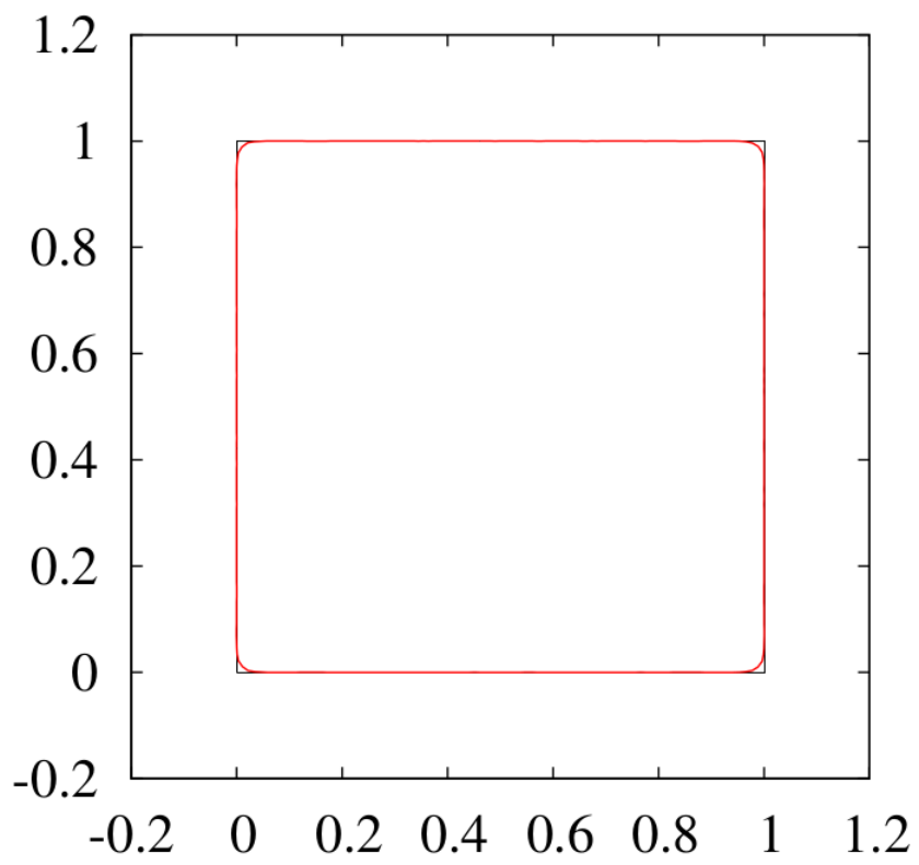
Refer to caption
(a) J∞hJ_{\infty}^{h} with H1H^{1} metric
Refer to caption
(b) J2hJ_{2}^{h} with Euclidean metric
Refer to caption
(c) J∞hJ_{\infty}^{h} with Euclidean metric
Refer to caption
(d) J2hJ_{2}^{h} with H1H^{1}-metric
Figure 5: Comparison of final shapes

All implementations were carried out within the FEniCS Software package [10]. The quadratic program (110) is solved with the python package cvxopt; cf. [1].


Figure 6: x-axis number of iterations and y-axis values J2h​(Ωn)J_{2}^{h}(\Omega_{n})

References

  • [1] M. S. Andersen, J. Dahl, and L. Vandenberghe. Cvxopt: A python package for convex optimization, version 1.1.8. preprint, 2016.
  • [2] P. Beremlijski, J. Haslinger, M. Kočvara, and J. Outrata. Shape optimization in contact problems with Coulomb friction. SIAM J. Optim., 13(2):561–587, 2002.
  • [3] E. Casas. Control of an elliptic problem with pointwise state constraints. SIAM J. Control Optim., 24(6):1309–1318, 1986.
  • [4] F. H. Clarke. Optimization and nonsmooth analysis, volume 5 of Classics in Applied Mathematics. Society for Industrial and Applied Mathematics (SIAM), Philadelphia, PA, second edition, 1990.
  • [5] C. Clason. L∞L^{\infty} fitting for inverse problems with uniform noise. Inverse Problems, 28(10):104007, 18, 2012.
  • [6] C. Clason, K. Ito, and K. Kunisch. Minimal invasion: an optimal L∞{\rm L}^{\infty} state constraint problem. ESAIM Math. Model. Numer. Anal., 45(3):505–522, 2011.
  • [7] M. C. Delfour and J.-P. Zolésio. Shapes and geometries, volume 22 of Advances in Design and Control. Society for Industrial and Applied Mathematics (SIAM), Philadelphia, PA, second edition, 2011. Metrics, analysis, differential calculus, and optimization.
  • [8] V. F. Dem′yanov and V. N. Malozëmov. Einführung in Minimax-Problem. Akademische Verlagsgesellschaft Geest & Portig K.-G., 1975. German translation.
  • [9] M. Eigel and K. Sturm. Reproducing kernel hilbert spaces in pde constrained shape optimisation. preprint.
  • [10] FEniCS Project - Automated solution of Differential Equations by the Finite Element Method, http://fenicsproject.org.
  • [11] K. Gröger. A W1,pW^{1,p}-estimate for solutions to mixed boundary value problems for second order elliptic differential equations. Math. Ann., 283(4):679–687, 1989.
  • [12] T. Grund and A. Rösch. Optimal control of a linear elliptic equation with a supremum norm functional. Optim. Methods Softw., 15(3-4):299–329, 2001.
  • [13] A. Habbal. Nonsmooth shape optimization applied to linear acoustics. SIAM J. Optim., 8(4):989–1006 (electronic), 1998.
  • [14] R. Haller-Dintelmann, C. Meyer, J. Rehberg, and A. Schiela. Hölder continuity and optimal control for nonsmooth elliptic problems. Appl. Math. Optim., 60(3):397–428, 2009.
  • [15] J. Haslinger and R. A. E. Mäkinen. Introduction to shape optimization, volume 7 of Advances in Design and Control. Society for Industrial and Applied Mathematics (SIAM), Philadelphia, PA, 2003. Theory, approximation, and computation.
  • [16] J. Haslinger, J. V. Outrata, and R. Pathó. Shape optimization in 2D contact problems with given friction and a solution-dependent coefficient of friction. Set-Valued Var. Anal., 20(1):31–59, 2012.
  • [17] C. Heinemann and K. Sturm. Shape optimization for a class of semi-linear variational inequalities. preprint.
  • [18] A. Henrot and M. Pierre. Variation et optimisation de formes, volume 48 of Mathématiques & Applications (Berlin) [Mathematics & Applications]. Springer, Berlin, 2005. Une analyse géométrique. [A geometric analysis].
  • [19] M. Hintermüller and A. Laurain. Optimal shape design subject to elliptic variational inequalities. SIAM J. Control Optim., 49(3):1015–1047, 2011.
  • [20] A. Laurain and K. Sturm. Distributed shape derivative via averaged adjoint method and applications. accepted in ESAIM Mathematical Modelling and Numerical Analysis.
  • [21] C. Meyer, L. Panizzi, and A. Schiela. Uniqueness criteria for the adjoint equation in state-constrained elliptic optimal control. Numer. Funct. Anal. Optim., 32(9):983–1007, 2011.
  • [22] J. Sokołowski. Shape sensitivity analysis of variational inequalities. In Shape optimization and free boundaries (Montreal, PQ, 1990), volume 380 of NATO Adv. Sci. Inst. Ser. C Math. Phys. Sci., pages 287–319. Kluwer Acad. Publ., Dordrecht, 1992.
  • [23] J. Sokołowski and J.-P. Zolésio. Shape design sensitivity analysis of plates and plane elastic solids under unilateral constraints. J. Optim. Theory Appl., 54(2):361–382, 1987.
  • [24] J. Sokołowski and J.-P. Zolésio. Introduction to shape optimization, volume 16 of Springer Series in Computational Mathematics. Springer, Berlin, 1992. Shape sensitivity analysis.
  • [25] K. Sturm. Minimax Lagrangian approach to the differentiability of nonlinear PDE constrained shape functions without saddle point assumption. SIAM J. Control Optim., 53(4):2017–2039, 2015.
  • [26] K. Sturm. On shape optimization with non-linear partial differential equations. PhD thesis, Berlin, Technische Universität Berlin, Diss., 2015.
  • [27] D. Werner. Funktionalanalysis. Springer-Verlag, Berlin, 5th extended edition, 2005.