An Empirical Study of Online Packet Scheduling Algorithms
Abstract
This work studies online scheduling algorithms for buffer management, develops new algorithms, and analyzes their performances. Packets arrive at a release time , with a non-negative weight and an integer deadline . At each time step, at most one packet is scheduled. The modified greedy (MG) algorithm is 1.618-competitive for the objective of maximizing the sum of weights of packets sent, assuming agreeable deadlines. We analyze the empirical behavior of MG in a situation with arbitrary deadlines and demonstrate that it is at a disadvantage when frequently preferring maximum weight packets over early deadline ones. We develop the MLP algorithm, which remedies this problem whilst mimicking the behavior of the offline algorithm. Our comparative analysis shows that, although the competitive ratio of MLP is not as good as that of MG, it performs better in practice. We validate this by simulating the behavior of both algorithms under a spectrum of simulated parameter settings. Finally, we propose the design of three additional algorithms, which may help in improving performance in practice.
1 Introduction
Efficient buffer management at a network router is a critical issue that motivates the online packet scheduling problem. Kesselman et al. [13] introduce a buffer management delay model and give algorithms to minimize end-to-end delay. We adopt a similar model to analyze the empirical behavior of the modified greedy (MG) algorithm introduced in [12], and propose new algorithms that do not have as strong worst-case guarantees, yet perform better in our simulated settings.
Model.
For simplicity, we investigate a network router with two nodes. Studying a two node router is a first step towards understanding more complicated and realistic models. In § 7 we briefly discuss possible model modifications. At each integer time step, packets are buffered upon arrival at the source node, then at most one packet is chosen from the buffer to be sent to the target node. A packet (,,) arrives at a release date , has a non-negative weight , and needs to be sent by an integer deadline . A packet not sent by expires, and is dropped from the buffer. The objective of a packet-scheduling algorithm is to maximize its weighted throughput, , defined as the total weight of packets sent by . It is easy to relate our model to an online version of the classical offline unit-job scheduling problem where the input is a set of unit-length jobs, each specified by a similar triple (,,) and the objective is to maximize weighted througput, that is the total weight of jobs that are processed before their deadlines.
Parameters.
We will typically be generating our input according to some type of distribution. Let denote the number of time steps during which the system can generate arriving packets, and let denote an arrival rate. We choose values for and . Then at each integer time step , we first generate the number of arriving packets according to a Poisson distribution with rate . For each arriving packet, we set and generate from a uniform (integer) distribution . To find , we first generate , a time to expire, from a uniform (integer) distribution , and set . We call this Model 1. We also consider a bimodal distribution for with weights and , respectively, for two distinct distributions centered on different means and call this Model 2. Although a network may induce correlations between packets, we use i.i.d. distributions as a first step in modeling the behavior of our algorithms.
In order to evaluate the performance of an online scheduling algorithm (A), we use an offline algorithm (OFF) for comparison, which given all future arrivals and packet characteristics, is able to statically find the optimal solution (e.g. using maximum-weight bipartite matching). Its solution gives the highest possible throughput the system can achieve. The online algorithm is k-competitive if on any instance is at least 1/k of on this instance. The smallest k for which an algorithm is k-competitive is called the competitive ratio [3]. According to [11], will be at most 2 for any algorithm that uses a static priority policy. In this paper, we will simulate the online algorithm and evaluate the ratio /. The average of these ratios across each batch of simulations will be denoted by , where is the corresponding online algorithm.
Related Work.
The literature is rich with works that acknowledge the importance of buffer management and present algorithms aiming at better router performance. Motivated by [13], [7] gives a randomized algorithm, RMIX, while [4] proves that it remains -competitive against an adaptive-online adversary. Many researchers attempt to design algorithms with improved competitive ratios. The best lower bound on the competitive ratio of deterministic algorithms is the golden ratio [11, 5]. A simple greedy algorithm that schedules a maximum-weight pending packet for an arbitrary deadline instance is 2-competitive [11, 13]. Chrobak et al. [8] introduce the first deterministic algorithm to have a competitive ratio strictly less than 2, namely 1.939. Li et al. [15] use the idea of dummy packets in order to design the DP algorithm with competitive ratio at most 1.854. Independently, [10] gives a 1.828-competitive algorithm. Further research considers natural restrictions on packet deadlines with hopes of improving the competitive ratio. One type of restriction is the agreeable deadline model considered in [12], i.e. deadlines are (weakly) increasing in their release times. Motivated by a more general greedy algorithm, [7], that schedules the earliest-deadline pending packet with weight at least of the maximum-weight pending packet, [12] develop the MG algorithm which will be described in § 2. In other models, researchers enforce the FIFO discipline using a model where packets have no deadlines and the buffer is finite. One of the earliest such algorithms is the FIFO preemptive model studied by [2]. Works such as [9, 14, 16] adopt similar ideas. We do not consider the FIFO discipline in this paper.
Our Contribution.
We observe that while MG is -competitive for the case of agreeable deadlines, it may not be the best option to apply in practice. We demonstrate the undesirable performance of MG under certain scenarios, e.g. frequently preferring maximum weight (late deadline) packets over early deadline ones. Our proposed MLP algorithm remedies this drawback, as it outperforms MG on most simulated instances. However, we are able to develop hard instances to prove that MLP does not provide better worst-case guarantees, whereas on those instances MG would produce the same results as an offline solution. Contrasting the advantages of MG and MLP motivates us to explore further algorithmic adjustments which may improve performance, at least in practice, as supported by our preliminary analysis. Finally, we justify that a two-node model with an infinite buffer is a sufficient model for our analysis. Moreover, extending the model to multiple nodes or imposing a threshold on the capacity of the buffer does not significantly alter the performance of the online algorithms.
2 Modified Greedy Algorithm (MG)
MG is a -competitive deterministic online algorithm for the agreeable deadline model [12]. It focuses on two packets at each time step: the earliest deadline non-dominated packet (i.e. maximum weight among all earliest-deadline packets) and the maximum weight non-dominated packet (i.e. earliest deadline among all maximum-weight packets in the buffer). Packet is chosen if () and is chosen otherwise. While [12] consider an agreeable deadline model, we relax this assumption and explore MG in a more general setting.
MG analysis.
Although MG has the best competitive ratio among deterministic online algorithms, we believe that by better understanding MG, we can improve on it in practice. Intuitively, if MG, at early stages, chooses packets with longer deadlines (due to higher weights) over those with early deadlines, then as time passes, many early packets expire while most of the heavy later-deadline packets will have already been sent. Therefore, the algorithm may resort to choosing packets with even smaller weights, thereby wasting an opportunity to send a higher weight packet that has already expired. We, hence, explore the decisions made by MG by observing its relative frequency of choosing over .
In order to consider a diverse set of instances, we set to 200 and define ranges [0.7,20], [1,20] and [1,40] for , and , respectively. Under the assumptions of Model 1, we run a batch of 200 simulations each for 8000 sampled parameter combinations. Given each parameter combination, we calculate the relative frequency of choosing over and average the frequencies over to obtain the empirical probability of , denoted by .

We suspect that when is high, especially if expires at later deadlines, MG will be at a major disadvantage. Figure 1 plots vs. , where each curve corresponds to a fixed level for . In general, increases with and . The decreasing curve slope implies that is more sensitive to lower values of . Further analysis shows that at any level of , MG will choose h over e at most 66% of the time. We also observe that regardless the average number of packets in the buffer, if is small (less than 3), the event of interest occurs at most 40% of the time.


From this probability analysis, we conclude that unless or are small, MG tends to choose packet too frequently. To show that this property may ”fire back”, we construct Scenario 1, forcing MG to favor later deadlines. We reuse the data of the generated packets above and adjust the weight of each packet by multiplying it by its deadline. We let MG run on the new data and plot against different parameters. Figure 2 depicts lower ratios for the new dataset. While originally increased with , it now decreases with and . does not affect the performance much. A gradient boosted tree predictive model (i.e. a sequence of decision tree models where the next model is built upon the residuals of the previous one) shows that is the most important factor under Scenario 1, as it accounts for 30% of the variability in the model.
3 Mini LP Algorithm (MLP)
Description.
In light of the previous analysis, we develop a new online algorithm that is more likely to send early deadline packets. The mini LP Algorithm (MLP) runs a ”mini” assignment LP at each time step in order to find the optimal schedule for the current content of the buffer, assuming no more arrivals. Assuming is the number of packets in the buffer at current time , we search for the packet with the latest deadline () and set a timeline from = 0 to . We then solve the following optimization problem, where is the weight of packet and is 1 if packet is sent at time and 0 otherwise:
MLP then uses the optimal solution to send the packet that receives the first assignment, i.e. the packet for which =1, while the rest of the schedule is ignored and recomputed in subsequent time steps.
3.1 Initial Analysis
Similar to the MG analysis, we compute and are interested in its behavior as the load varies. A way to measure load is to define the average number of packets in the buffer as , which is a byproduct of . We expect higher at low , since the online algorithm would not have many packets to choose from and hence, is more likely to choose the same packet as the offline algorithm at each time step. However, we expect to decrease as increases, since the discrepancy between online and offline solutions increases. To test this, we sample parameter combinations from , and , and run a batch of 1000 simulations per combination.

Figure 3 plots vs. and interestingly shows a dip-shaped graph: starts at a very high value (), decreases as expected with increasing until eventually it increases again, thereby forming a dip, and finally converges to 1. Our claim is true at first, when is relatively low, as the first range for is quite sensitive ( vs. 2.8 makes a difference). However, when increases, the problem loses its sensitivity. An explanation for such behavior may be that as increases (with increasing ), we are more likely to have multiple packets achieving maximum weight, in which case both the online and offline algorithms are likely to choose those packets and have less discrepancy between their choices, especially if the weight or deadline ranges are not wide enough. We conclude that when the system is heavily or lightly loaded, both algorithms perform well. The dip happens in the interesting area. Consequently, we will investigate how the dip moves and what the effect of parameter choices will have on such graph.
3.2 Parameter Effect on MLP Behavior
Changing the parameters to generate different graphs did not change the structure of the dip-shaped graph that we have seen in Figure 3. Nonetheless, the dip gets narrower/wider and shifts to the left/right, as parameters change. In this section, we will only focus on a restricted range for the values of , namely 0.7 to 10. However, we believe that the restriction does not mask any interesting results, since MLP converges at higher values of , as we have seen before. Therefore, a heavily loaded system is not significant for our analysis.
Arrival Rates.
The graph inevitably depends on , as it directly affects , i.e. the x-axis. However, does not have a direct effect on the shape of the graph. By tuning the range for , we are able to “zoom in” onto the dip area and monitor the behavior more accurately where the system is neither lightly nor heavily loaded. The range for such sensitive values is on average between 1.3 and 4.2. Figure 1(a) (in the appendix) zooms in on the dip where is most sensitive.
Weight Ranges.
The range of the weights moves the dip to the right (left), as it gets narrower (wider). Very narrow ranges (i.e. low values for ) are the most influential. As increases, its impact decreases. In fact, this result seems intuitive and one can see an example in Figure 1(b) where the weight range is designed to be very narrow ( is set at 2). Some experimentation led us to the explanation of this phenomenon: When there are few options for weights, both algorithms converge together. Let’s say weights are only 1 and 2, then the higher the , the more likely we will have packets of weight 2. In this case both algorithms find the optimal choice to be the packet with higher weight (we don’t have much choice here so it must be 2). Hence, both behave alike. We note that it is not in particular the range of weights that has this effect but rather the number of distinct weights available, i.e. choosing between weights 1 and 2 vs. 100 and 200, would depict the same behavior.
Time Period and Deadline Range.
and have a combined effect. Figures 1(c) and 1(d) give two examples: Allowing a longer timeline results in a second but higher dip and slows down convergence, such that suddenly higher values of become slightly more interesting. Meanwhile lower values (combined with shorter ’s) result in a graph with one sharp dip as well as much faster convergence to 1.
3.3 Influence of maximum-weight packets
The motivation of MLP was mainly to remedy the drawback we observed for MG when later deadline packets are preferred. Therefore, it is essential to verify that MLP outperforms MG under Scenario 1. In fact, one-sided 99% confidence intervals (CI) imply that is at most 91.98% while is at most 96.28%. The difference in performance between both algorithms increases with . Figure 4(a) shows the behavior of against for both algorithms. While MLP is not influenced by under this scenario, the performance of MG gets worse as increases. A 99% two-sided CI for , denoted by , is (1.0443,1.0552), implying that MLP produces a total weight at least 4.43% more than that of MG under this scenario. Better performance is observed with higher or lower , but does not seem to influence the algorithms’ performances.


4 Comparative Analysis
In this section, we contrast the behavior of MG and MLP under a spectrum of parameter settings. We are interested in the behavior of the ratios against our parameters and expect MLP to perform better in our simulations. The general procedure for our simulations is based on sampling parameter combinations from a predefined parameter space. we impose the following parameter range restrictions: , , and (Scenario 2). For each combination, we run MG, MLP (5 times each) and the offline algorithm in order to obtain values for , , as well as . Detailed steps for simulations are given in § 0.A.1.
4.1 Ratio behavior w.r.t. model parameters
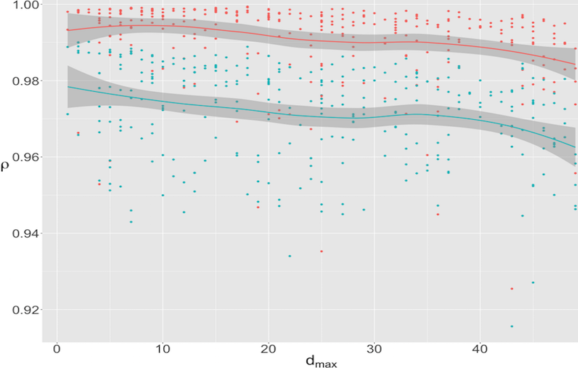
Comparing and against values of implies that on average MLP outperforms MG (Figure 4(b)). As increases, both algorithms perform better. A 99% one-sided CI for is (0,0.9734), implying that we are 99% confident that is at most 97.34% of , while the one-sided CI for is (0,0.9926). In Figure 0.B.2.1, it is evident that MG produces a wider spread of the ratios. All else constant, the performance of each algorithm improves with higher , lower or higher , whereas it is not influenced by the values of .


Figure 5(a) plots vs. , colored by . For very small ’s, there is the possibility that MLP and MG perform similarly; in some cases, MG outperforms MLP, regardless of the value of . However, for large , MLP tends to outperform MG. A 99% two-sided CI for is , implying that we are 99% confident that is at least 1.88% more than . However, both algorithms have similar performance as the upper bound of the CI shows that is at most 2.16% more. Whether this is beneficial depends on the use case as well as time constraints (see § 5). § 0.A.2 presents a brief analysis where we construct gradient booted tree predictive models on the ratios for inference purposes.
4.2 Changing the distribution of
So far, we have only considered uniform distributions, however, real inputs are more complicated. Here we make one step towards modeling more realistic inputs and consider a that follows a bimodal distribution of two distinct peaks (recall Model 2); with probability , is and with probability , is . We restrict our parameters to the following ranges: ,

, and (Scenario 3). We choose a bimodal distribution because these distributions are often hard for scheduling algorithms. Indeed, we see that the results for Scenario 3 are slightly different.
While MG performs worse with increasing , improves with and still outperforms (Figure 6).The graph for resembles a dip-shaped graph, yet we find this dip to be entirely above the confidence interval of . All else constant, neither algorithm is influenced greatly by any of the parameters , or . Figure 5(b) plots vs. , where lighter points correspond to longer ’s. For very small , MLP and MG perform similarly. In some cases, MG outperforms MLP, regardless of the value of . However, for large , a 95% CI shows that MLP outperforms MG by at least 2.80% and at most 3.30%.
5 Hard Instances

The previous analysis presents evidence that MLP gives better competitive ratios than MG. An index plot (Figure 7) of and shows that, for the same instances, MLP not only outperforms MG, but also gives a ratio of 1 for most of the instances that are hard for MG. However, it would be incorrect to conclude that MLP always has a better competitive ratio than MG. In fact, we are able to create hard instances for MLP where it performs worse than MG. A small example is given in Table 1.
| Packet(r,d,w) | MLP | MG | Offline |
|---|---|---|---|
| Assign to | |||
| Assign to | Assign to | ||
| Assign to | Assign to | Assign to | |
| 2 | 2 |
For , we can easily see that MLP is 2-competitive, while on those instances is 1. However, such worst-case instances may be rare and our results show that MLP performs better on a varied set of data. On the other hand, MG, which bases its decisions on simple arithmetic, is simpler than MLP which solves an LP at each time step. In our experiments, MLP was as much as 140 times slower than MG. In the next section, we consider some modifications to take advantage of the strengths of both approaches.
6 Algorithm Modifications
In an attempt to find faster solutions, we introduce some possible algorithmic modifications. Preliminary results show slight performance improvement when these modifications are applied. However, more analysis is needed to verify the results and choose the best parameters for improvement.
6.1 The Mix and Match Algorithm (MM)
Algorithm.
The Mix and Match Algorithm (MM) combines both MG and MLP. At each time step, MM chooses to either run MG or MLP-according to . If is high, then by previous analysis, MG and MLP each converges to 1 (assuming Model 1), and MM runs MG, as it is faster and has a competetive ratio that is as good as that of MLP. If is low, MM runs MLP, as it is more accurate and the running time is also small since is low. To distinguish between ”high” and ”low”, we define a threshold . Although MM suffers from the same limitations as MLP, it might still be preferred due to its smaller computation time.
Simulation.
We set to 200 and define ranges [0.7,15], [1,30], [1,23] and [5,20] for , , and , respectively. We compare under different values of . We also average , use the same simulations to run MG and average . We take the ratio of both averages and plot it against (Figure 8). Preliminary results show that that for small , the algorithm, at higher , does slightly worse than at lower . However, the opposite is true for large .


Future work.
Further ideas are needed to set the optimal choice for . We may want to look at the percentage of times the algorithm chose to run MG over MLP in order to monitor time complexity. Another idea would be to take hard instances of MG into consideration and explore how to derive conditions such that the algorithm switches to MLP in such cases.
6.2 The Learning Modified Greedy Algorithm (LMG)
Algorithm.
MG and MLP are memoryless [12], i.e. the assignment of packets at time uses no information about assignments at times . We introduce a non-memoryless modification to MG. Recall that MG compares to . In the learning MG (LMG) algorithm, we try to make use of the past performance of MG, in order to replace by a more suitable divisor. If defines the frequency of learning, then every steps, we calculate the throughput at the current divisor, . Then we search for a divisor, , which lies in the vicinity of , but yields higher throughput using the previous data. Finally, we proceed with the new divisor , given by () for some smoothing factor . The detailed procedure for LMG is given below:
Step 0.
Set the frequency of learning, , i.e. the time window needed to define a learning epoch. Then run MG and use the following procedure every steps in order to replace the divisor, , by a sequence of better divisors as follows:
- 1.
Generate a sequence of divisors ’s starting at the current divisor and having jumps of , without going below 1 or above 2.5. For instance, if =1.62, we generate the following sequence: 1.02, 1.07, , 1.57, 1.62, 1.67, , 2.47.
- 2.
Start with the throughput associated with and move left in our generated sequence. At each , we calculate the throughput of MG on the previous data. We keep moving to subsequent divisors as long as there is an increase in throughput. Next, we do the same with divisors to the right. Given a left endpoint and a right one, we choose the divisor associated with the higher throughput and denote it by . Some toy examples are shown in Table 2. For simplicity, we only observe the weighted throughput for four values of .
Thruput/ 1.57 =1.62 1.67 1.72 Case 1 2 4 4 2 1.62 Case 2 2 4 2 6 1.62 Case 3 6 4 5 7 1.72 Case 4 4 4 4 4 1.62 Case 5 6 4 3 7 1.57 Table 2: Examples for choosing - 3.
The new divisor is given by smoothing with , i.e. for some
Simulation.
We use the same parameter space as in § 6.1. We set and for simplicity, . The choice for in general must ensure that the process of finding an optimal divisor does not generate a jumpy sequence of divisors. Our analysis for 8000 sampled scenarios shows that LMG outperforms MG 83.3% of the time. The range of the improvement is [-0.6%, 2.8%], implying that LMG brings as much as 2.8% increase in the ratio over MG. Performance is worse when the sequence of ’s is around 1.618, implying that LMG is picking up on some noise and should not change the divisor.
Future work.
One can avoid this noise by statistically testing and justifying the significance of changing the divisor. In terms of time complexity, LMG is not slower than MG, as it can be done while the regular process is running. Finally, no direct conclusion is made about a threshold on the number of packets beyond which LMG is particularly effective. Further analysis could yield such conclusion, thereby indicating at which instances LMG should be used.
6.3 The Second Max Algorithm (SMMG)
Algorithm.
Inspired by the dummy packet (DP) algorithm discussed in [15] for cases of non-agreeable deadlines, we realize the importance of extending the comparison to a pool of more than two packets. The key idea in SMMG is to prevent the influence a single heavy packet may have on subsequent steps of the algorithm. We try to find an early-deadline packet that is sufficiently large compared to the heaviest packet. We set a value for and the iterations are as follows:
- 1.
If MG chooses , send and STOP.
- 2.
Else find the earliest second largest packet in the buffer, denoted by .
- 3.
If and , send . Else send .
The intuition here is that sending packet is always a good choice, so we need no modification. However, we limit over-choosing packet by finding the earliest second-largest packet . The concern is that keeping in the buffer may bias the choice of the packets. Hence, we send , if its weight is significant enough, in order to eliminate its influence and keep the possibility of sending for a subsequent iteration (as expires after ). To evaluate that is significant enough, we verify that it exceeds (otherwise, we should have sent e), as well as , a proportion of . Note that for instance, if , it means that SMMG is very conservative allowing the fewest modifications to MG.
Simulation.
We use the same parameter space as in § 6.1 and try values for as follows: 0.65, 0.75, 0.85, 0.95. Figure 9 plots the improvement of SMMG over MG ( - ) vs. , colored by . As expected, the lower the value of , the bigger the deviation from MG. At very low , we see that applying SMMG is not useful, however, as increases, the improvement remains positive. At all values of , the improvement is at its highest when is between 8 and 12 packets. Hence, SMMG is useful when is in the vicinity of the interval between 4 and 17. Whether this is a significant result, depends on the nature of our problem. Even if , the minimum improvement within that interval is around 0.8%. However, the maximum improvement is 1.5% (at ).

7 Model Discussion
The two-node model with no buffer limitations clearly does not capture all aspects of realistic network models. Thus, in this section, we will consider a multi-node model and also the case of finite buffer capacity.
Multi-node model.
In the previous analysis, we only considered a two-node-system, namely the source and the target nodes. In order to understand multinode systems, we consider first a three node system, that is a system of two tandem queues and see how the throughput behaves.
Assume the arrival rate at node 1 is and that each packet has to be sent to visit node 2 then reach node 3 by its deadline. Some packets will be lost at node 1, as they expire before being sent. Node 2 will, hence, have less traffic. We assume as before that we can send at most one packet per node at each time step. Within this framework, we are interested to know whether this setup results in a deterministic online algorithm of better performance. Our simulation shows that node 2 either has the same throughput as node 1 or lower. After tracing packets, it turns out that this is a fairly logical result because node 2 only receives packets from node 1. The packet will either expire at stage 2 or go through to node 3. So the throughput can only be at most the same as that of node 1.
The following minor adjustment slightly improves the performance at node 2: Each arriving packet has a deadline to reach node 3, denoted by . We introduce a temporary deadline for that packet to reach node 2 by . This modification guarantees that we only send packets to node 2 if after arriving at node 2 there is at least one more time unit left to its expiration in order to give the packet a chance to reach node 3. Here is a trivial example: A packet arrives with deadline 7, i.e. it should arrive at node 3 by 7. Before the adjustment it was possible for this packet at time 7 to be still at node 1 and move to node 2, then be expired at node 2 and get lost. After the adjustment, this packet will have a deadline of 6 for node 2. So if by time 6, the packet hasn’t been sent yet, it gets deleted from the buffer of node 1 (one time step before its actual deadline). This adjustment improved the throughput of node 2 to be almost equal to that of node 1 because the arrival rate at node 2 is at most 1 (at most one packet is sent from node 1 at each time step). So node 2 is usually making a trivial decision of sending the only packet it has in its buffer.
In conclusion, our model implicitly imposes a restriction on the maximum possible throughput at internal nodes, hence, making the multi-node model, where only one packet is sent at each time step, an uninteresting problem. In § 8, we give, however, a few future directions for more interesting extensions.

Finiteness of Buffer.
Throughout this paper, we chose not to put any restrictions on the buffer capacity and therefore we now look to verify whether the finiteness of the buffer has a major effect on the algorithm performance and its bounds. We run a set of experiments where, given , we find the corresponding buffer size , such that the probability of exceeding is one in a million. We create an index plot for the ratio of (Figure 10) and conclude that imposing a buffer size is unnecessary. Even when , the buffer size needs to be about 1.53 as much, i.e. 153. Furthermore, for the interesting values of used throughout this report, a buffer size of around 30 would be more than sufficient. We conclude that imposing a capacity limit on the buffer is not necessary as choosing a reasonable buffer size should not affect the algorithm’s performance.
8 Conclusion
In this paper, we consider several old and new packet scheduling algorithms. By analyzing the empirical behavior of MG, we observe that MG chooses packet over too frequently. We therefore develop a new algorithm, MLP, which mimics the offline algorithm and gives higher attention to early deadline packets. We then show that on a wide variety of data, including uniform and bimodal distributions, MLP is slower, but has a better empirical competitive ratio than MG. (This is in contrast to the worst-case analysis where MG has a better competitive ratio.)
We then propose three new algorithms that may offer an improvement in empirical performance, as they combine features of both algorithms. MM, at each time step, chooses between using MG or MLP in order to make a decision on the packet to send. LMG learns from previous behavior to correct the divisor used in MG, while SMMG is motivated by the idea of influential packets in extending the comparison to a pool of three packets, namely , and . The improvements for these algorithms are small, yet encouraging for further analysis. Moreover, it is important to consider extensions for the network model and run the algorithms on one where induced correlations are captured by more realistic distributions that are not i.i.d. Contrasting the behavior of any of the algorithms mentioned in this paper on an actual router, rather than a simulated environment, would also be important to consider.
Several interesting future directions remain. One important extension would be a multi-node model. We showed how the straightforward extension does not yield much insight but other extensions may be more interesting. For example, one could have nodes that process at different rates; this would prevent the first node from being an obvious bottleneck. Another possibility is to allow feedback, that is, if a packet expires somewhere in the multi-node system, it could return to the source to be resent. A final possibility is for each packet to have a vector of deadlines, one per node, so that different nodes could be the bottleneck at different times.
Acknowledgments
The authors would like to thank Dr. Shokri Z. Selim and Javid Ali.
References
- [1] S. Albers and M. Schmidt. On the performance of greedy algorithms in packet buffering. SIAM Journal on Computing (SICOMP), 35(2):278–304, 2005.
- [2] N. Andelman, Y. Mansour, and A. Zhu. Competitive queuing polices for QoS switches. In Proceedings of the 14th Annual ACM-SIAM Symposium on Discrete Algorithms (SODA), pages 761–770, 2003.
- [3] A. Borodin and R. El-Yaniv Online Computation and Competitive Analysis. Cambridge University Press, 1998
- [4] M. Bieńkowski, M. Chrobak, and Ł. Jeż. Randomized algorithms for buffer management with 2-bounded delay. In Proceedings of the 6th Workshop on Approximation and Online Algorithms (WAOA), pages 92–104, 2008.
- [5] F. Y. L. Chin and S. P. Y. Fung Online Scheduling with Partial Job Values: Does Timesharing or Randomization Help? Algorithmica, 37(3): 149–164, 2003
- [6] F. Y. L. Chin and S. P. Y. Fung Improved competitive algorithms for online scheduling with partial job values. Theoretical computer science, 325(3): 467-478,2004.
- [7] F. Y. L. Chin, M. Chrobak, S. P. Y. Fung, W. Jawor, J. Sgall, and T. Tichy. Online competitive algorithms for maximizing weighted throughput of unit jobs. Journal of Discrete Algorithms, 4(2):255–276, 2006.
- [8] M. Chrobak, W. Jawor, J. Sgall, and T. Tichy Improved Online Algorithms for Buffer Management in QoS Switches In Proceedings of 12th European Symposium on Algorithms (ESA), pages 204–215, 2004.
- [9] M. Englert and M. Westermann Lower and Upper Bounds on FIFO Buffer Management in QoS Switches. In Proceedings of 14th Annual European Symposium on Algorithms (ESA), pages 352–363, 2006.
- [10] M. Englert and M. Westermann Considering Suppressed Packets Improves Buffer Management in QoS Switches. In Proceedings of 18th Annual ACM-SIAM Symposium on Discrete Algorithms (SODA), pages 209–218, 2007.
- [11] B. Hajek. On the competitiveness of online scheduling of unit-length packets with hard deadlines in slotted time. In Proceedings of 2001 Conference on Information Sciences and Systems (CISS), pages 434–438, 2001.
- [12] Ł. Jeż, F. Li, J. Sethuraman, and C. Stein. Online scheduling of packets with agreeable deadlines. ACM Transactions on Algorithms (TALG), 9(1):5, 2012.
- [13] A. Kesselman, Z. Lotker, Y. Mansour, B. Patt-Shamir, B. Schieber, and M. Sviridenko. Buffer overflow management in QoS switches. SIAM Journal on Computing (SICOMP), 33(3):563–583, 2004.
- [14] A. Kesselman, Y. Mansour, R. van Stee. Improved Competitive Guarantees for QoS Buffering. Algorithmica, 43:63–80, 2005.
- [15] F. Li, J. Sethuraman, and C. Stein. Better online buffer management. In Proceedings of the 18th Annual ACM-SIAM Symposium on Discrete Algorithms (SODA), pages 199–208, 2007.
- [16] Z. Lotker and B. Patt-Shamir Nearly Optimal FIFO Buffer Management for DiffServ. In Proceedings of the 21st ACM Symposium on Principles of Distributed Computing (PODC), pages 134–142, 2002.
Appendix 0.A Appendix
0.A.1 General Procedure for Simulations in § 4
Our simulations try to avoid any initial bias by starting with a nonempty system. This is the role of the variable which ”warms up” the system; that is the simulation will take place for time steps before collecting any data. This warmup period allows the content of the buffer to adjust to normal running conditions for the system. The general simulation procedure is as follows:
- 1.
Identify a parameter range for the parameters , , and .
- 2.
Randomly select a parameter combination within the parameter space.
- 3.
Set .
- 4.
Generate inputs for time steps using the chosen parameter combination.
- 5.
Find the optimal offline solution, for the last T steps only, i.e. sum of weights of packets sent from to and let that be our .
- 6.
Run MG and record the weighted throughput for the last T steps only.
- 7.
Repeat Step 6 five times and let our be the average weighted throughput over the five runs.
- 8.
Run MLP and record the weighted throughput for the last T steps only.
- 9.
Repeat Step 8 five times and let our be the average weighted throughput over the five runs.
- 10.
Compute , , as well as .
- 11.
Repeat Steps 2-10 500 times.
Note that the input generation in Step 3 has been described in § 1.
0.A.2 Predictive Model
We construct a gradient boosted tree (GBT) predictive model on the results for inference purposes. The predictors were , , , and whether MG or MLP were used and the response was of the respective algorithm. In terms of variable importance (as measured by the model and stated as a percentage), and turn out to be the two most important parameters.
| Feature | MLP? | MG? | ||||
|---|---|---|---|---|---|---|
| Variable Importance | 41% | 15% | 8% | 3% | 17% | 16% |
Figure 1(a) plots both model parameters for each of the algorithms, and colors them by . This allows us to view the behavior of the ratio in a multivariate manner: We see here that there is a point where the ratios tend to level off, approximately (as can be seen by the constancy of the colors) around and . We looked to see if this was perhaps a result of the average number of packets in the buffer but saw slight correlation, as is evident in Figure 1(b).
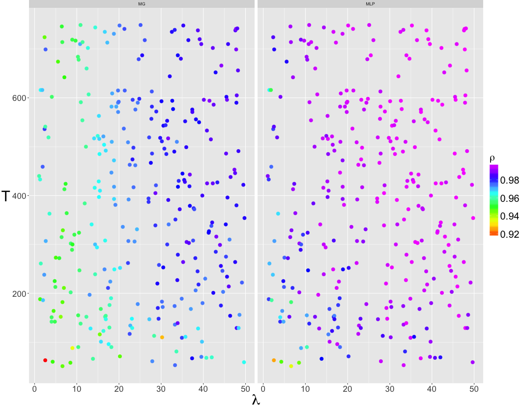


Next, we perform predictions from the model for a much larger range of and (risking extrapolation issues). In Figure 2(b), is well behaved for large values of and : there seems to be a dip but that may be due to randomness. Furthermore, the ratios do not dip as sharply as for MG in Figure 2(d). This leads us to investigate more the behavior of for larger values of , which leads us to Scenario 4 where values for are extended to and the same analysis is run for MG.
The results for the behavior of vs. shows an increasing performance under Scenario 4. We are 99% confident that is at most 98.69% of . Plots against other parameters show that the performance of MG, all else constant, would get better with larger or lower and only slightly better for larger . A gradient boosted tree predictive model again shows that and are the two most important variables. As and get larger, gets better.
Appendix 0.B Figures
0.B.1 Parameter Effect on MLP Behavior


0.B.2 (red) and (green) vs. different parameters