Matrix product states for invariant quantum spin chains
Abstract
A systematic and compact treatment of arbitrary invariant spin- quantum chains with nearest-neighbour interactions is presented. The ground-state is derived in terms of matrix product states (MPS). The fundamental MPS calculations consist of taking products of basic tensors of rank 3 and contractions thereof. The algebraic calculations are carried out completely by making use of Wigner calculus. As an example of application, the spin-1 bilinear-biquadratic quantum chain is investigated. Various physical quantities are calculated with high numerical accuracy of up to 7 digits. We obtain explicit results for the ground-state energy, entanglement entropy, singlet operator correlations and the string order parameter. We find interesting crossover phenomena in the correlation lengths.
1 Introduction
Matrix product states (MPS) continue to attract scientific attention either as a subject in its own right, or as realizations [1, 2] in density matrix renormalization group (DMRG) studies [3]-[6]. In the condensed matter community, the interest in such states developed with the discovery of AKLT models with exact ground-states of the type of MPS with finite dimensional auxiliary space [7, 8], also called valence bond solids. Generalizations including anisotropic models followed in [9]-[15], where especially in [11]-[13] the formulation as matrix product states was used. The models [7, 8], despite their fine-tuned interactions, were found to be representatives of ‘typical’ systems. The naturally appearing boundary degrees of freedom added even more interest to the MPS states as they realize topological order [16, 17]. On the practical side, the MPS allowed for a variational treatment of the ground-state of a given Hamiltonian [1, 2, 18]-[21] resulting in the current understanding of DMRG techniques, see e.g. [6]. Finally, in the literature on integrable lattice systems MPS states appear where the local tensor is called vertex operator [32]-[34].
In this paper we are interested in the fundamental implementation of Lie algebra symmetries in MPS with as a most important example, however with arbitrary spin- in the quantum space. By doing this, we are convinced that any calculation can be performed more efficiently than without use of the symmetry. To give an example of this reasoning we like to remind again of the AKLT model [7, 8]. By use of a transfer matrix formalism, all correlation functions of the state can be calculated from the eigenstates and eigenvalues of the transfer matrix. In the case of AKLT, the transfer matrix is nothing but a product of two symbols. The eigenstates themselves are nothing but symbols, and the eigenvalues are symbols. All of these objects are ‘tabulated’ and no actual calculation is needed, just the right identification is necessary.
The use of Lie algebra symmetries in DMRG calculations has some history [35] -[40]. In the paper [39] two of the current authors have started to formulate the local tensors of MPS and various associated objects like transfer matrices in a invariant manner by use of Wigner calculus. The work [39] was restricted to spin- in the quantum space. In this paper we present the generalization to arbitrary spin- and report on concrete applications to the spin-1 bilinear-biquadratic quantum chain which we investigate in a large part of the Haldane phase. In addition to the generalization over [39] we managed to formulate less intricate graphical rules for the construction of the basic components of MPS calculations. We believe that such transparent rules are also essential for calculations in the higher dimensional case of tensor network states, see for instance [22]-[25] and especially for variational treatments [26]-[31].
The paper is organized as follows. In Sect. 2 we shortly summarize the tensor calculus of MPS and introduce the invariant local objects based on Wigner’s symbols. Many objects are presented in diagrammatical manner and are based on graphs with three-pointed vertices. The graphical rules are formulated and explicit formulas for various kinds of transfer matrices are given. We treat general nearest-neighbour couplings, entanglement entropy and string order. In Sect. 3 we present explicit results from numerical variational calculations for the spin-1 bilinear-biquadratic chain. The results are compared with numerical data of the literature. In Sect. 4 we present our conclusions.
2 Realization of invariance
We consider the class of matrix-product states
| (1) |
where is a square matrix with some auxiliary (index) space . The matrix entries of are elements of a local quantum space which we take as the th copy of a spin- space .
The -invariance of is guaranteed if the objects are invariant tensors in , where is the dual space to . We treat the case of a finite dimensional , however with arbitrary dimensionality. This space will consist of a direct sum over irreducible spin- representations where . Each may appear an arbitrary number of times , in which case we label the different orthogonal mupltiplets by an integer . The space is spanned by orthogonal states where the magnetic quantum number varies from to in integer steps.
Let us consider in any spin multiplet from the first factor space, any spin multiplet from the second factor space, and the (only) spin multiplet of the third space. Disregarding scalar factors, there is at most one way of coupling these multiplets to a singlet state. The coupling coefficients are known as symbols and the desired singlet is
| (5) |
We are going to use graphical rules for the construction of invariant tensors like . We associate with any graph consisting of three-pointed stars (vertices) and closed or open directed lines (bonds) an -invariant tensor:
- •
Bonds carry an angular momentum label and a label where summation over is implied. The label is usually explicitly shown, is not. [In case we are dealing with several multiplets of type we number those with an integer and label the bond with .]
- •
Bonds evaluate to factors
in case of a closed bond,
in case of an open bond with outgoing arrow,
in case of an open bond with ingoing arrow.
- •
Vertices evaluate to a factor where , , are read off from the bonds of the vertex in anti-clockwise manner. The sign of each entry in the symbol is determined by the arrow direction: and for ‘out’ and ‘in’.
The number of open bonds is equal to the rank of the tensor. Note that due to the symmetries of the symbols an arrow on a closed bond with associated label may be reverted resulting in a factor .
In Fig. 1 we show the graphical depiction of and its dual which is obtained by changing ket-vectors into bra-vectors and vice versa.

A general invariant tensor can be written as superposition of these elementary singlets
| (6) |
with suitable coefficients . Note that does not appear as index of as is always fixed and unique (for this reason no has been introduced either). Due to the symmetry of symbols with respect to exchange of two columns
| (7) |
we conclude that
| (8) |
with globally fixed , is a sufficient condition for parity invariance. Note that is always integer.
Also note that only few combinations need to be considered: if the triangle condition is violated, the three multiplets can not couple to a singlet.
2.1 Norm and transfer matrix
Next, we want to calculate the norm and the expectation value of the Hamiltonian in the thermodynamic limit. The computation leads to
| (9) |
where is the dual of and the contraction over the third space is implicitly understood in . Hence is a linear map . A quite explicit expression for is given in a mixed algebraic and graphical manner in Fig. 2.

For the computation of the norm we employ the transfer matrix trick yielding for the r.h.s. of (9)
| (10) |
where the sum is over all eigenvalues of . Obviously, in the thermodynamic limit only the largest eigenvalue(s) contribute. The corresponding left and right eigenstates are denoted by and .
The computation of the leading eigenvalue is facilitated by the singlet nature of the leading eigenstate. There are not many independent singlet states in . A multiplet in and a multiplet in couple to a singlet iff (with arbitrary and ). The (normalized) singlet is given by
| (11) |
Graphically, this singlet is depicted by a link carrying an arrow pointing from the to the space, a label in the middle and , at the respective ends.
The action of the transfer matrix onto singlets produces singlets with matrix elements
| (12) |
For this calculation the identity depicted in Fig. 3 has been used (where for the derivation of (12) is to be used).

The total dimension of is , but the singlet subspace is much lower dimensional: . Due to the still high dimensionality, the diagonalisation in the singlet space has to be done numerically.
In order to give full meaning to the graphical operations in Fig. 3 we complement our rules by
- •
Isolated (directed) bonds carry an angular momentum label and evaluate to a product of the factors
for the end with outgoing arrow,
for the end with ingoing arrow.
- •
Concatenations of two or more graphs correspond to contractions over pairs of open bonds and naturally lead to identifications of the labels that are carried by the joined bonds.
Note that these rules are consistent with the above rule for the factor contributed by a closed bond. Also note that indices identifying different multiplets of the same type appear on the bonds and usually pertain to the entire bond. The only exception are the singlet states represented by arcs with possibly different labels and at the ends.
2.2 Nearest-neighbour couplings
We are interested in the spin- Heisenberg chain with most general nearest-neighbour interaction. The corresponding Hamiltonian can be written in two alternative ways
| (13) |
either with a polynomial of degree applied to the scalar product of the nearest-neighbour spin vectors, or as a superposition of many projection operators onto nearest-neighbour spin multiplets . The operator is given in terms of symbols like
| (19) | |||||
and is graphically depicted in Fig. 4.

We want to determine the matrix-product state with minimal expectation value of the total Hamiltonian . Due to translational invariance the expectation value of a single projector acting on sites 1 and 2 needs to be calculated leading to
| (20) |
is a modified transfer matrix acting in , is the (normalized) leading eigenstate of the transfer matrix and we kept the only term that dominates in the thermodynamical limit. Hence
| (21) |
For the explicit expression of we use the calculus of Wigner symbols. is obtained from the multiplication of with two tensors and two . The underlying graph contains two triangles that allow for an explicit evaluation of the internal sums over the ‘magnetic’ quantum numbers. In this way, triangles are reduced to vertices times symbols. Details of these calculations are shown in Fig. 5.

The final result of these calculations is given in Fig. 6.
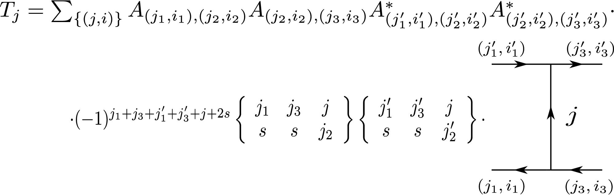
2.3 Entanglement
Next, we consider a finite segment of length inside a very long quantum chain. The reduced density matrix is obtained from the total density matrix by taking the trace over all local spaces except for those at sites
| (22) |
This object can be written in terms of basis states on the sites
| (23) |
Note that these states are usually not orthonormalized, but satisfy
| (24) |
where and are the left and right leading eigenstates of the transfer matrix , and we have defined the matrices and .
The matrix elements of the reduced density matrix can then be given in the form
| (25) |
Hence, the reduced density matrix in an orthonormalized basis is isomorphic to . Furthermore, the entanglement entropy is twice the entropy of the matrix .
2.4 Hidden order
Next, we are interested in the computation of long-range string order [16, 17], i.e. ‘hidden order’. Due to symmetry, the standard two-point spin-spin-correlators decay to zero for large separations of the operators and . However, the expectation value of the spin operators times does not necessarily vanish. It is known to be non-zero for the Haldane phase of the Heisenberg chain. By use of transfer matrices we find
| (26) |
where the modified transfer matrices and are defined similar to the standard tranfer matrix with the additional action of the spin operators on the physical space: and . In case of we may apply an important simplification rewriting the action of on the third component of as the action of on the first two components of . This is due to (actually ) invariance: on the r.h.s. of (5) only terms with contribute. Now these operators on the horizontal bonds cancel pairwise in the product of the many transfer matrices, except for one factor on the left and one on the right end. These factors may then be associated in the general bookkeeping with the resulting in
| (27) |
where are identical to with the additional action of and in the and case. For large separation we find the leading contribution
| (28) |
just from knowing the leading eigenstate of .
Working with the modified transfer matrices leads to the insertion of a vertex ( symbol) into the vertical line in the graphical depiction in Fig. 2 as well as associating minus signs with the lower left and right bonds. The additional vertex has two bonds with spin- and a third label with spin- (and for dealing with the component of the spin operator).
We need matrix elements of in the singlet subspace. This result looks like (12) with two additional factors on the r.h.s. A factor stems from treating the spin operators by symbols and takes care of the normalization . The second factor originates from the summation over internal variables of a graph where a triangle is reduced to a star yielding a symbol. For we obtain the factor
| (29) |
where the last sum evaluates to for half odd integer and simply for integer .
3 Results
For the nearest-neighbour spin- quantum chain with bilinear and biquadratic interaction
| (30) |
we performed calculations for . In the auxiliary space we used alternatively purely integer spin multiplets and purely half-odd integer spin multiplets. In the diagrams we show results for , , , (=0 for ) where is the number of independent spin- multiplets. This corresponds to a 46-dimensional auxiliary space. Taking into account a gauge freedom already described in [39] we have to deal with 41 variational parameters. The actual calculations have been carried out in Maple 13. The minimum in energy was found by the built-in optimization routine and also – with same result – by a simple gradient procedure.
For we found a ground-state energy per site of which is off by (only) from the best known numerical value of [41]. Our result for the string order parameter is to be compared with by [41]. We obtain for the entanglement entropy and for the correlation length of singlet operators . Our value for the entropy compares well with that reported in [43].
At the model is critical and the accuracy of the data in the above approximation is worse. Still the results for the ground-state energy , the expectation values of the projectors onto nearest-neighbour singlets and triplets and deviate only by from the exactly known values , and [42].
At our results reproduce the known analytical facts about the AKLT model [7, 8]. Here only the correlation parameter of a single multiplet in the auxiliary space with itself is enough to realize the exact ground state with , string order parameter and entanglement entropy . All other correlation (variational) parameters are 0. The state with a single spin-1/2 multiplet on each bond is of course the VBS state where the symbol at the vertex produces a spin-1 by symmetrization, and the product of two vertices in the auxiliary space (contraction) corresponds to antisymmetrization of two spin-1/2 objects.
In the course of our numerical experiments we found that the same state can be constructed also by integer spin multiplets in the auxiliary space. This can be understood analytically: One needs for instance one spin-0 and one spin-1 multiplet. The spin-0 and spin-1 couple with weight and the spin-1 with itself with ‘weight’ .
The dependence of the ground-state energy and of the expectation values of the projection operators , on is quite smooth – not to say boring – see Fig. 7 a). The true behaviour of the entanglement entropy would show a singularity at , but only rises to the finite value of in our treatment due to the finite number of multiplets. Likewise, the finite string order , see Fig. 7 b), decreases upon approaching , but does not drop to exactly 0. We calculated the correlation lengths of singlet correlation functions from the next-leading eigenvalues of the transfer matrix . The next-leading positive and negative eigenvalues result in the correlation lengths and . For approaching both lengths increase, in an exact treatment they would diverge. At some the lengths show a crossover. Interestingly, for this point the papers [44, 1] reported a softening of an excitation gap at momentum .


We believe, that this is not a coincidence. In any case, the implication of the crossover is that for singlet correlators will generically show oscillating asymptotics, see Fig. 8 a), and for the asymptotics will be uniformly decaying. However, matrix elements may be of different orders of magnitude and may obscure this behaviour at finite distances, see Fig. 8 b) where only at sufficiently large distances the oscillations set in.
The dependence of on is not very smooth. This need not be a numerical artefact. Especially for at a crossover of another high-lying negative eigenvalue looks responsible for the non-monotonous dependence on . Finally, we like to mention that for all singlet correlators are zero.


4 Conclusion
In this paper we presented a most economical formulation of general invariant MPS with arbitrary spin- in the quantum space. The basic objects for the calculation of expectation values of nearest-neighbour interactions and of correlation functions appear as contractions over products of fundamental tensors of rank 3. The contractions involve internal sums over ‘magnetic quantum numbers’ which were evaluated explicitly by use of Wigner calculus. The results of these algebraic calculations were presented in invariant manner in terms of and symbols.
The usefulness of the invariant formulation was demonstrated at the example of the spin-1 bilinear-biquadratic quantum chain directly in the thermodynamical limit. For a large part of the Haldane phase we determined by variational calculations the ground-state energy, the expectation values of projection operators on nearest-neighbour singlet and triplet spaces, the entanglement entropy, string order and singlet operator correlations as well as their leading correlation lengths.
The achieved accuracy is probably more than acceptable for practical purposes. Our numerical calculations were done in Maple 13 and resulted in an accuracy of for the ground-state energy of the strictly bilinear spin-1 Heisenberg chain. These results were obtained for 5, 4, 2, 1 copies of spin-, , , and multiplets in the auxiliary space which in total is 46-dimensional.
In future work we want to develop a ‘normal’ program code to do faster calculations and to deal with larger dimensional auxiliary spaces. Ultimately, and by making use of the gained experience with the calculus of MPS, we intend to tackle tensor-network calculations.
Acknowledgments.
The authors would like to thank Y. Öz and J. Sirker for valuable discussions. The authors gratefully acknowledge support by Deutsche Forschungsgemeinschaft under project Renormierungsgruppe KL 645/6-3. AK acknowledges support by CNRS and the hospitality of Université Pierre et Marie Curie where the final stages of the presented work were carried out.
References
References
- [1] Stellan Ostlund und Stefan Rommer, Thermodynamic limit of the density matrix renormalization for the spin-1 Heisenberg chain, Phys. Rev. Lett. 75, p.3537 (1995)
- [2] Stefan Rommer und Stellan Ostlund, A class of ansatz wave functions for 1D spin systems and their relation to DMRG, Phys. Rev. B 55, 2164 - 2181 (1997)
- [3] S. R. White, Density matrix formulation for quantum renormalization groups, Phys. Rev. Lett. 69, 2863 (1992)
- [4] S.R. White und R. Noack, Real-space quantum renormalization groups, Phys. Rev. Lett. 68, 3487 1992 ; S.R. White, Density matrix formulation for quantum renormalization groups, ibid. 69, 2863 1992 ; S.R. White, Density-matrix algorithms for quantum renormalization groups, Phys. Rev. B 48, 10 345 1993
- [5] E. Jeckelmann, Dynamical density-matrix renormalization-group method, Phys. Rev. B 66, 045114 (2002)
- [6] U. Schollwöck, The density-matrix renormalization group, Rev. Mod. Phys. 77, 259 (2005)
- [7] I. Affleck, T. Kennedy, E. H. Lieb and H. Tasaki, Phys. Rev. Lett. 59,799 (1987).
- [8] I. Affleck, T. Kennedy, E. H. Lieb and H. Tasaki, Comm. Math. Phys. 115, 477 (1988).
- [9] M. Fannes, B. Nachtergaele and R. F. Werner, Exact antiferromagnetic ground states of quantum spin chains, Europhys. Lett. 10, 633 (1989).
- [10] M. Fannes, B. Nachtergaele and R. F. Werner, Finitely correlated states on quantum spin chains, Comm. Math. Phys. 144, 443 (1992).
- [11] A. Klümper, A. Schadschneider, J. Zittartz: Equivalence and solution of anisotropic spin-1 models and generalized - fermion models in one dimension J. Phys. A 24, L955-L959 (1991)
- [12] A. Klümper, A. Schadschneider, J. Zittartz: Groundstate properties of a generalized VBS-model Z. Phys. B87, 281-287 (1992)
- [13] C. Lange, A. Klümper, J. Zittartz: Exact ground-states for antiferromagnetic spin-one chains with nearest and next-nearest neighbour interactions, Z. Phys. B 96, 267 (1994)
- [14] A. K. Kolezhuk, H.-J. Mikeska, Finitely Correlated Generalized Spin Ladders, Int. J. Mod. Phys. B, Vol.12, 2325-2348 (1998)
- [15] A. K. Kolezhuk, H.-J. Mikeska, Mixed spin ladders with exotic ground states, Eur. Phys. J. B v.5, 543 (1998)
- [16] M. den Nijs, K. Rommelse, Phys, Rev. B 40, 4709 (1989)
- [17] H. Tasaki, Phys. Rev. Lett. 66, 798 (1991)
- [18] A. Schadschneider, and J. Zittartz: Variational study of isotropic spin-1 chains using matrix-product states,Ann. Phys. Vol. 507, (1995) 157–163
- [19] A. Kolezhuk, R. Roth, und U. Schollwöck, First Order Transition in the Frustrated Antiferromagnetic Heisenberg S=1 Quantum Spin Chain, Phys. Rev. Lett. 77, 5142 (1996)
- [20] A. Kolezhuk, R. Roth, und U. Schollwöck, Variational and density-matrix renormalization-group studies of the frustrated antiferromagnetic Heisenberg S=1 quantum spin chain, Phys. Rev. B 55, 8928 (1997)
- [21] A. K. Kolezhuk, H.-J. Mikeska, Shoji Yamamoto, Matrix product states approach to the Heisenberg ferrimagnetic spin chains, Phys. Rev. B 55 (1997) R3336
- [22] A. Klümper, H. Niggemann, J. Zittartz: Quantum phase transitions in spin-3/2 systems on the hexagonal lattice– optimum ground-state approach, Z. Phys. B 104, 103 (1997)
- [23] H. Niggemann, A. Klümper und J. Zittartz: Ground-state phase diagram of a spin-2 antiferromagnet on the square lattice, Euro. Phys. J. B 13, 15 (2000)
- [24] V. Murg, F. Verstraete, und J. I. Cirac: Exploring frustrated spin systems using projected entangled pair states, Phys. Rev. B 79, 195119 2009
- [25] G. Evenbly and G. Vidal: Frustrated Antiferromagnets with Entanglement Renormalization: Ground State of the Spin-1 Heisenberg Model on a Kagome Lattice, PRL 104, 187203 (2010)
- [26] T. Nishino, K. Okunishi, Y. Hieida, N. Maeshima und Y. Akutsu, Self-consistent tensor product variational approximation for 3D classical models, Nucl. Phys. B575, 504 (2000)
- [27] J. J. Gararcia-Ripoll, J. I. Cirac, P. Zoller, C. Kollath, U. Schollwöck, J. von Delft, Variational ansatz for the superfluid Mott-insulator transition in optical lattices, Opt. Express 12, 42 (2004)
- [28] A. Isacsson und O. F. Syljuasen, Variational treatment of the Shastry-Sutherland antiferromagnet using projected entangled pair states, Phys. Rev. E 74, 026701 (2006)
- [29] V. Murg, F. Verstraete, und J. I. Cirac, Variational study of hard-core bosons in a two-dimensional optical lattice using projected entangled pair states, Phys. Rev. A 75, 033605 (2007)
- [30] A. W. Sandvik und G. Vidal, Variational Quantum Monte Carlo Simulations with Tensor-Network States, PRL 99, 220602 (2007)
- [31] H. C. Jiang, Z. Y. Weng, und T. Xiang, Accurate Determination of Tensor Network State of Quantum Lattice Models in Two Dimensions, PRL 101, 090603 (2008)
- [32] M. Jimbo, K. Miki, T. Miwa, und A. Nakayashiki, Correlation functions of the XXZ model for , Phys. Lett. A 168 (1992), 256.
- [33] M. Jimbo und T. Miwa, Quantum KZ equation with and correlation functions of the XXZ model in the gapless regime, J. Phys. A 29 (1996), 2923.
- [34] Herman E. Boos, Frank Göhmann, Andreas Klümper, Junji Suzuki, Factorization of multiple integrals representing the density matrix of a finite segment of the Heisenberg spin chain, J. Stat. Mech. 0604 (2006) P001
- [35] J. Dukelsky, M. A. Martin Delgado, T. Nishino and G. Sierra, Equivalence of the Variational Matrix Product Method and the Density Matrix Renormalization Group applied to Spin Chains, Europhys. Lett. 43 (1998) 457.
- [36] J. M. Roman, G. Sierra, J. Dukelsky and M. A. Martin-Delgado, The Matrix Product Approach to Quantum Spin Ladders., J. Phys. A: Math. Gen. 31 (1998) 9729.
- [37] McCulloch I P and Gulácsi M, The non-Abelian density matrix renormalization group algorithm, Europhys. Lett. 57 852 (2002)
- [38] Jorge Dukelsky and Stuart Pittel: The Density Matrix Renormalization Group for finite Fermi systems, Rep. Prog. Phys. 67, 513-552 (2004)
- [39] Andreas Fledderjohann, Andreas Klümper, Karl-Heinz Mütter, Diagrammatics for invariant matrix product states, J. Phys. A: Math. Theor. 44 (2011) 475302, arXiv:1107.5258
- [40] Andreas Weichselbaum, Non-abelian symmetries in tensor networks: A quantum symmetry space approach, Annals of Physics 327, 2972–3047 (2012)
- [41] Steven R. White and David A. Huse, Numerical renormalization-group study of low-lying eigenstates of the antiferromagnetic Heisenberg chain, Phys. Rev. B 48, (1993)
- [42] Andreas Klümper, Dominic Nawrath, Junji Suzuki: Correlation functions of the integrable isotropic spin-1 chain: algebraic expressions for arbitrary temperature, J. Stat. Mech. P08009 (2013)
- [43] Xiao-Yan Deng, Long-Juan Kong, and Ling Qiang:String order and degenerate entanglement spectrum of and Heisenberg bond-alternating chains,Eur. Phys. J. B 87 (2014), 247
- [44] J. Oitmaa, J. B. Parkinson and J. C. Bonner J. Phys. C 19, L595 (1986)