A new dynamical instability in asymptotically Anti-de-Sitter spacetime
Abstract
We present fully dynamical solutions to Einstein-scalar theory in asymptotically Anti-de-Sitter spacetime with a scalar potential containing particularly rich physics. Depending on one parameter in the potential we find an especially interesting regime, which exhibits a dynamically unstable black brane, already at zero momentum, while nevertheless having positive specific heat. We show this using the non-linear dynamics, and give a clear interpretation in terms of the spectrum of linearized perturbations. Our results translate directly to their dual strongly coupled non-conformal field theories, whereby we in particular provide two mechanisms to obtain equilibration times much larger than the inverse temperature.
1. Introduction Holography has led to crucial qualitative lessons for the physics of real-time dynamics and equilibration in strongly coupled quantum theories, such as the fast applicability of hydrodynamics, within a time of , with being the temperature of the plasma [1, 2, 3, 4]. These studies were mostly performed in a scale invariant setting, where the scaling is automatic. Much richer physics can be expected for theories without scale invariance or relativistic symmetry, which is an active topic of current research both in relation to quark-gluon plasma [5, 6, 7, 8, 9, 10, 11, 12] and condensed matter systems [13, 14, 15]. In this Letter we present such a new lesson, where we find stationary phases which display a dynamical instability at zero momentum, whereby the time scale of the instability can be much larger than the inverse temperature.
Einstein-scalar theory in the context of non-conformal holographic QCD was first introduced in [16, 17] (see also [18]). In this Letter we follow Refs. [19, 20], which introduced a simple potential that could mimic the thermodynamics of QCD as in [16, 17], but differs from the latter in the small asymptotics. Our potential contains an exponent that controls the deviation of the dual field theory from the conformal limit . In particular, it was shown in [21] that the dual theory exhibits a confinement-deconfinement transition for the choice . However, most of the detailed analysis focused on the particular case of , which is the most realistic choice for the QCD phenomenology[22].
In this Letter we initiate a detailed study of the regime by solving Einstein-scalar equations of motion both in a time-independent and a time-dependent setting, to determine respectively the thermodynamics, and the process of thermalization in the corresponding dual field theory. We discover a new critical value beyond which a new, qualitatively different regime arises. This value depends on the mass of the scalar that corresponds to the scaling dimension of the scalar operator , and the quoted value is for . For smaller it is known that there is a minimum temperature, at fixed source, above which there is a large, stable branch and an unstable branch which has negative specific heat and a vanishing entropy for large temperature. For larger we find that both branches at the minimum temperature have positive specific heat. Interestingly, the solution with smaller black brane area still has growing entropy for large but is nevertheless dynamically unstable and hence contains an exponentially growing mode. Lastly, as the temperature goes towards the minimum temperature both solutions coalesce, whereby the relaxation time diverges. We illustrate all these features by tuning our initial conditions such that the evolution first relaxes onto the unstable black brane solution, after which it decays into the stable black brane.
We hence provide two mechanisms to violate the typical scaling of the equilibration time. Firstly, as mentioned it is possible to increase the source to its maximum value, where the equilibration time diverges. Secondly, at smaller sources it is possible to fine-tune the initial conditions such that the evolution stays at the unstable time-independent solution for a time .


Our results also provide an interesting addition to the literature on the instability of black branes [23]. In particular, it is different from a Gregory-Laflamme type instability [24]. These type of instabilities are often present in black rings and black branes in more than four dimensions and involve the break up of the ring or brane into smaller parts, which can be thermodynamically favourable. Curiously, the thermodynamics of black holes crucially relies on Hawking’s computation [25], which requires quantum mechanics. It is hence not obvious that the classical Einstein equations would contain a dynamical instability, if a thermodynamic instability is present (see however [26]). Nevertheless, a black brane always contains a dynamical instability if a thermodynamic instability is present, as conjectured by Gubser and Mitra in [27, 28] (see also [29, 30, 31]) and recently proved in [32].
Our example is reminiscent of the models studied in [33]. This reference also has hairy black holes in Einstein-scalar theory, which are not unique when specifying all conserved charges. They note that these non-unique stationary solutions can be unstable to flow towards other solutions. Since this does not necessarily involve conserved charges this instability can also occur at zero momentum and with positive specific heat, such as the example presented here in a fully non-linear dynamical setting 11 1 It is an interesting question if a dynamical instability also implies a thermodynamic instability. Naively our example is thermodynamically stable with respect to all conserved charges, but as noted in [33] it may be more natural to consider a wider definition of thermodynamics which includes non-conserved charges..


2. The model and results Our confining model is given by the Einstein-scalar action
| (1) |
which includes a scalar field dual to a scalar operator with scaling dimension . We follow [19, 20] and take
| (2) |
which near reads
| (3) |
such that we have a negative cosmological constant with , and the mass of the scalar is independent of the value of the free parameter . In this Letter we present results for and . In order to solve dynamical simulations it is convenient to use the characteristic formulation of general relativity [35, 1, 36], which is achieved by using a metric ansatz
| (4) |
whereby we study homogeneous solutions which only depend on time and AdS radial coordinate . The equations of motion following from (1) are written down in i.e. [5], and lead to a near-boundary expansion for as
| (5) |
where is a time-independent source for the scalar, is the normalizable mode undetermined by the near-boundary analysis and is a gauge freedom left in (4), which we use to fix the apparent horizon at . The normalizable mode has dimension 3 and hence in principle scales as for fixed . However, due to the anomalous logarithmic term in (5) also includes a term . The expectation value of can be obtained through holographic renormalization [37, 5]:
| (6) |
where we again notice that this includes an anomalous term proportional to . As always, there is a scheme dependence in the renormalization procedure whereby finite counterterms can shift (6) without affecting the physics presented.
Lastly, we have to specify initial conditions. Both for numerics and for presentation it is convenient to treat the near-boundary behavior of analytically and hence define as
| (7) | |||||
where and by construction . The initial conditions are then fully specified by for and the normalizable mode of , which we call .
During the evolution we furthermore keep track of the spectrum of linearized perturbations around the metric with scalar field, the so called quasi-normal modes (QNM). We solved for the QNM spectrum by constructing gauge invariant observables from the linearized equations [38, 39] and used spectral methods to solve the eigenvalue problem and hence obtain the QNM spectrum [40].
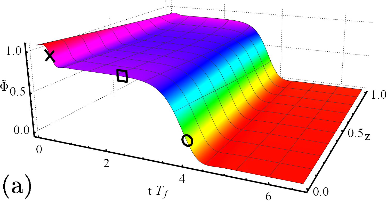
The main result is captured in Fig. 1(a), where we take 22 2 We chose this value because this is the maximum value where the spectrum of fluctuations around the vacuum is still well defined [17]. , , and . Strikingly, the time evolution of this initial profile goes through three phases. First, within a time of the inverse temperature, the system relaxes to a time-independent state. This state is however unstable, and after a time depending on how close the unstable state was reached the system relaxes again to the stable solution. We stress that we needed to fine-tune our initial condition to remain at the unstable state for a long time, but apart from this fine-tuning this phenomenon is fully generic, provided 33 3 In practise this fine-tuning is done by increasing ; for values higher than the fine-tuned value the evolution looks like Fig. 3(c), which is easy to distinguish from Fig. 1(a) at late times and hence makes a binary search algorithm straightforward. Note that we have to fine-tune the coefficient of one QNM, so we just have to fine-tune one parameter instead of a function..
In Fig. 1(b) the three regimes are shown more clearly, first there is the decay to the unstable solution by the lowest two stable QNM of the unstable phase, which is dominant since we fine-tuned the coefficient of the unstable QNM to be small. Then there is a semi-stationary period where this small coefficient grows exponentially. Finally the solution exits the linear regime around the unstable solution and rings down in the linear regime around the stable solution. All three dominant modes are indicated in Fig. 2, as red QNMs around the unstable background (first phases) and around the stable background (blue). Note that the unstable QNM has vanishing real part, which is required [23]. It is reassuring to see all QNMs of the stable and unstable solutions meet at . It is interesting that the lowest QNM of the stable phase crosses the second QNM to meet the stable partner of the unstable QNM of the unstable phase.


Interestingly, for larger source we find the same features, up to a maximum source , as illustrated in Fig. 2 and 3 (a). At the unstable and stable branch merge, and the lowest QNM of both solutions has . This then naturally gives rise to an overdamped relaxation towards the equilibrium solution, which we show in Fig. 3 (b). Clearly, at this point the thermalization takes asymptotically longer than the standard with the temperature of the final state, which is an interesting novelty for non-conformal strongly coupled systems.
Lastly, we studied the unstable QNM at for different values of , which is presented in Fig. 4(a). As approaches the critical value 1.65 from above the imaginary part goes to zero and we hence again find a diverging relaxation time. We also verified that for smaller no instability is present at zero momentum.
We performed several numerical checks. All our simulations satisfy the constraint equation to better than precision (with the exception of Fig. 3(c)). We also compared the QNM spectrum with fits of the dynamical evolution when this was in the linear regime, which is a non-trivial check. Lastly, we used a thermodynamic code to construct the time-independent solution, which allowed us to study the equilibrium properties of both the stable and unstable solutions.
3. Discussion The thermodynamics of the stable and unstable phase is presented in Fig. 4(b) and (c), where we show the entropy and free energy versus the temperature (computed using the method of [43]). Indeed the unstable solution has smaller entropy than the stable solution, but this phase still consists of a large black hole, in the sense that the black hole grows as temperature grows. This stands in contrast with two other branches in our model, shown dashed, which includes a small black hole branch, smoothly connecting to the thermal gas phase as the temperature goes to infinity. This branches are more involved to study dynamically as they are thermodynamically unfavored, and we plan to report on this in future work.
As alluded to in the Introduction, one curious feature is that the solution shown in Fig. 1(a) is unstable already at zero momentum, in contrast to the standard Gregory-Laflamme type instability. This in particular allows for a positive specific heat and a positive speed of sound squared, as is clear from Fig. 4 (c). From a field theory point of view this instability is perhaps less dramatic, as the plasma need not break up, but evolves homogeneously to a different phase. Nevertheless, the scalar operator acquires a different expectation value, and the entropy can at least double for small .
Our results are very generic. For other dimensions, other scaling dimensions and other potentials with a large enough contribution we were able to find the unstable QNM at zero momentum. Also the inclusion of anisotropy in the metric (4) does not give rise to qualitative changes.
The unstable QNM found in Fig. 1 has an interesting alternative. When choosing instead of the coefficient of the unstable QNM changes sign, and hence starts growing exponentially instead of decreasing. This means the final stable configuration found in Fig. 1 will not be reached. Our numerics do not allow to determine the final endpoint of this type of evolution, of which the first moments are displayed in Fig. 5(c). This would be interesting for future study, whereby we note that our evolution starts with regular initial conditions, an apparent horizon and that our model satisfies the null energy condition.
Our results are most easily understood in terms of the QNM spectrum of both the stable (blue) and unstable solutions (red) on the complex plane, which we show as a function of again for in Fig. 5. Starting at the blue circle for large black holes with each QNM follows a blue trajectory until the maximum source . At this point the lowest QNM hits the origin and we show the other branch in red, ending again at with a red square. It is interesting to see the lowest QNM of the stable phase hits the imaginary axis and hence become overdamped, which is similar to QNMs in Lifshitz spacetimes [15].
Indeed non-conformal theories contain rich physics. The different
black brane solutions found contain a new dynamical instability
already at zero momentum. This new mechanism leads in
particular to a value of where the quasi-normal mode
frequency goes to zero and hence the relaxation time
diverges, which we showed to be a generic feature in non-conformal
strongly coupled theories.
Note added: while finalizing our draft, the paper [9] appeared on the arXiv that also reports dynamical instability at vanishing momentum in a similar gravitational setting. However the QNM they find has a small positive imaginary part, about 0.05.
Acknowledgments. We thank Alex Buchel, Steven Gubser, Phil Szepietowski, Takaaki Ishii, Luis Lehner, Michal Heller, Elias Kiritsis, David Mateos, Francesco Nitti and Chris Rosen for useful discussions. WS is supported by the U.S. Department of Energy under grant Contract Number DE-SC0011090. This work was supported by the Netherlands Organisation for Scientific Research (NWO) under VIDI grant 680-47-518, and the Delta-Institute for Theoretical Physics (D-ITP) that is funded by the Dutch Ministry of Education, Culture and Science (OCW).
References
- [1] P. M. Chesler and L. G. Yaffe, Phys.Rev.Lett. 102, 211601 (2009), arXiv:0812.2053 [hep-th] .
- [2] P. M. Chesler and L. G. Yaffe, Phys.Rev.Lett. 106, 021601 (2011), arXiv:1011.3562 [hep-th] .
- [3] M. P. Heller, R. A. Janik, and P. Witaszczyk, Phys.Rev.Lett. 108, 201602 (2012a), arXiv:1103.3452 [hep-th] .
- [4] M. P. Heller, D. Mateos, W. van der Schee, and D. Trancanelli, Phys.Rev.Lett. 108, 191601 (2012b), arXiv:1202.0981 [hep-th] .
- [5] T. Ishii, E. Kiritsis, and C. Rosen, JHEP 08, 008 (2015), arXiv:1503.07766 [hep-th] .
- [6] A. Buchel, M. P. Heller, and R. C. Myers, Phys. Rev. Lett. 114, 251601 (2015), arXiv:1503.07114 [hep-th] .
- [7] J. F. Fuini and L. G. Yaffe, JHEP 07, 116 (2015), arXiv:1503.07148 [hep-th] .
- [8] R. A. Janik, G. Plewa, H. Soltanpanahi, and M. Spalinski, Phys. Rev. D91, 126013 (2015), arXiv:1503.07149 [hep-th] .
- [9] R. A. Janik, J. Jankowski, and H. Soltanpanahi, (2016), arXiv:1603.05950 [hep-th] .
- [10] U. Gursoy, M. Jarvinen, and G. Policastro, JHEP 01, 134 (2016a), arXiv:1507.08628 [hep-th] .
- [11] Y. Du, S.-Q. Lan, Y. Tian, and H. Zhang, JHEP 01, 016 (2016), arXiv:1511.07179 [hep-th] .
- [12] M. Attems, J. Casalderrey-Solana, D. Mateos, I. Papadimitriou, D. Santos-Oliván, C. F. Sopuerta, M. Triana, and M. Zilhão, (2016), arXiv:1603.01254 [hep-th] .
- [13] W. Sybesma and S. Vandoren, JHEP 05, 021 (2015), arXiv:1503.07457 [hep-th] .
- [14] J. Brewer and P. Romatschke, Phys. Rev. Lett. 115, 190404 (2015), arXiv:1508.01199 [hep-th] .
- [15] U. Gursoy, A. Jansen, W. Sybesma, and S. Vandoren, (2016b), arXiv:1602.01375 [hep-th] .
- [16] U. Gursoy and E. Kiritsis, JHEP 0802, 032 (2008), arXiv:0707.1324 [hep-th] .
- [17] U. Gursoy, E. Kiritsis, and F. Nitti, JHEP 02, 019 (2008a), arXiv:0707.1349 [hep-th] .
- [18] C. Csaki and M. Reece, JHEP 05, 062 (2007), arXiv:hep-ph/0608266 [hep-ph] .
- [19] S. S. Gubser, A. Nellore, S. S. Pufu, and F. D. Rocha, Phys. Rev. Lett. 101, 131601 (2008), arXiv:0804.1950 [hep-th] .
- [20] S. S. Gubser and A. Nellore, Phys. Rev. D78, 086007 (2008), arXiv:0804.0434 [hep-th] .
- [21] U. Gursoy, E. Kiritsis, L. Mazzanti, and F. Nitti, Phys. Rev. Lett. 101, 181601 (2008b), arXiv:0804.0899 [hep-th] .
- [22] U. Gursoy, E. Kiritsis, L. Mazzanti, and F. Nitti, Nucl. Phys. B820, 148 (2009a), arXiv:0903.2859 [hep-th] .
- [23] R. A. Konoplya and A. Zhidenko, Rev. Mod. Phys. 83, 793 (2011), arXiv:1102.4014 [gr-qc] .
- [24] R. Gregory and R. Laflamme, Phys. Rev. Lett. 70, 2837 (1993), arXiv:hep-th/9301052 [hep-th] .
- [25] S. Hawking, Commun.Math.Phys. 43, 199 (1975).
- [26] H. S. Reall, Phys. Rev. D64, 044005 (2001), arXiv:hep-th/0104071 [hep-th] .
- [27] S. S. Gubser and I. Mitra, (2000), arXiv:hep-th/0009126 [hep-th] .
- [28] S. S. Gubser and I. Mitra, JHEP 08, 018 (2001), arXiv:hep-th/0011127 [hep-th] .
- [29] V. E. Hubeny and M. Rangamani, JHEP 05, 027 (2002), arXiv:hep-th/0202189 [hep-th] .
- [30] A. Buchel, Nucl. Phys. B731, 109 (2005), arXiv:hep-th/0507275 [hep-th] .
- [31] A. Buchel, Nucl. Phys. B820, 385 (2009), arXiv:0903.3605 [hep-th] .
- [32] S. Hollands and R. M. Wald, Commun. Math. Phys. 321, 629 (2013), arXiv:1201.0463 [gr-qc] .
- [33] J. J. Friess, S. S. Gubser, and I. Mitra, Phys. Rev. D72, 104019 (2005), arXiv:hep-th/0508220 [hep-th] .
- [34] It is an interesting question if a dynamical instability also implies a thermodynamic instability. Naively our example is thermodynamically stable with respect to all conserved charges, but as noted in [33] it may be more natural to consider a wider definition of thermodynamics which includes non-conserved charges.
- [35] H. Bondi, Nature 186, 535+ (1960).
- [36] W. van der Schee, Gravitational collisions and the quark-gluon plasma, Ph.D. thesis, Utrecht University (2014), arXiv:1407.1849 [hep-th] .
- [37] S. de Haro, S. N. Solodukhin, and K. Skenderis, Commun.Math.Phys. 217, 595 (2001), arXiv:hep-th/0002230 [hep-th] .
- [38] P. K. Kovtun and A. O. Starinets, Phys. Rev. D72, 086009 (2005), arXiv:hep-th/0506184 [hep-th] .
- [39] P. Benincasa, A. Buchel, and A. O. Starinets, Nucl. Phys. B733, 160 (2006), arXiv:hep-th/0507026 [hep-th] .
- [40] L. G. Yaffe, http://msstp.org/?q=node/289 .
- [41] We chose this value because this is the maximum value where the spectrum of fluctuations around the vacuum is still well defined [17].
- [42] In practise this fine-tuning is done by increasing ; for values higher than the fine-tuned value the evolution looks like Fig. 3(c), which is easy to distinguish from Fig. 1(a) at late times and hence makes a binary search algorithm straightforward. Note that we have to fine-tune the coefficient of one QNM, so we just have to fine-tune one parameter instead of a function.
- [43] U. Gursoy, E. Kiritsis, L. Mazzanti, and F. Nitti, JHEP 05, 033 (2009b), arXiv:0812.0792 [hep-th] .