Observability through matrix-weighted graph

Observability is one of the central concepts in systems theory which, for LTI systems, can be expressed in many seemingly different yet mathematically equivalent forms [7]. One alternative is the following. A pair $[C,\,A]$ is observable if $C(x_{1}(t)-x_{2}(t))\equiv 0$ implies $x_{1}(t)\equiv x_{2}(t)$, where $x_{i}(t)$ denote the solutions of two identical systems ${\dot{x}}_{i}=Ax_{i}$, $i=1,\,2$. Admittedly, this appears to be an uneconomical definition, for the implication therein employs two systems where one would have sufficed. The overuse, however, has a relative advantage: it points in an interesting direction of generalization. Namely, for a pair $[(C_{ij})_{i,j=1}^{q},\,A]$ the below condition suggests itself as a natural extension.

$\displaystyle C_{ij}(x_{i}(t)-x_{j}(t))\equiv 0\ \mbox{for all}\ (i,\,j)\implies x_{i}(t)\equiv x_{j}(t)\ \mbox{for all}\ (i,\,j)$

(1)

where $x_{i}(t)$ are the solutions of $q$ identical systems ${\dot{x}}_{i}=Ax_{i}$, $i=1,\,2,\,\ldots,\,q$. Aside from its theoretical allure, this particular choice of generalization is not without practical motivation; the condition (1) happens to be both necessary and sufficient for synchronization of certain arrays of oscillators. We give two examples in the sequel.

Coupled electrical oscillators. Consider the individual oscillator in Fig. 1, where $p$ linear inductors with inductances $m_{1},\,m_{2},\,\ldots,\,m_{p}>0$ are connected by linear capacitors with capacitances $k_{1},\,k_{2},\,\ldots,\,k_{p+1}>0$.

The node voltages are denoted by $z^{[\ell]}\in{\mathbb{R}}$. Letting $z=[z^{[1]}\ z^{[2]}\ \cdots\ z^{[p]}]^{T}$ the model of this system reads $K{\ddot{z}}+M^{-1}z=0$ where $M={\rm diag}(m_{1},\,m_{2},\,\ldots,\,m_{p})$ and

$\displaystyle K=\left[\begin{array}[]{ccccc}k_{1}+k_{2}&-k_{2}&0&\cdots&0\\ -k_{2}&k_{2}+k_{3}&-k_{3}&\cdots&0\\ 0&-k_{3}&k_{3}+k_{4}&\cdots&0\\ \vdots&\vdots&\vdots&\ddots&\vdots\\ 0&0&0&\cdots&k_{p}+k_{p+1}\end{array}\right]\,.$

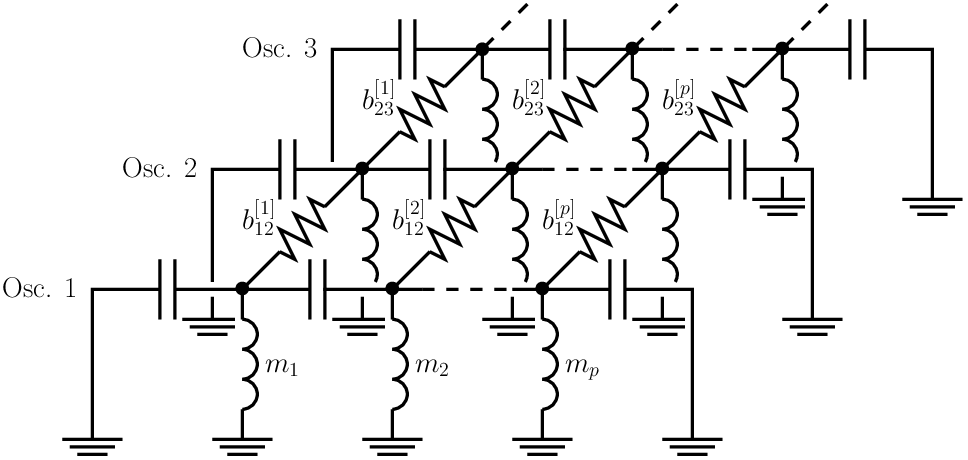
Let now an array be constructed by coupling $q$ identical oscillators in the arrangement shown in Fig. 2. If we let $z_{i}\in{\mathbb{R}}^{p}$ denote the node voltage vector for the $i$th oscillator and $b_{ij}^{[\ell]}=b_{ji}^{[\ell]}\geq 0$ be the conductance of the resistor connecting the $\ell$th nodes of the oscillators $i$ and $j$, we obtain $K{\ddot{z}}_{i}+M^{-1}z_{i}+\sum_{j=1}^{q}B_{ij}({\dot{z}}_{i}-{\dot{z}}_{j})=0$, where $B_{ij}={\rm diag}(b_{ij}^{[1]},\,b_{ij}^{[2]},\,\ldots,\,b_{ij}^{[p]})$. Denoting by $x_{i}=[z_{i}^{T}\ {\dot{z}}_{i}^{T}]^{T}$ the state of the $i$th system we can then rewrite the coupled dynamics as

$\displaystyle{\dot{x}}_{i}=\left[\begin{array}[]{cc}0&I_{p}\\ -K^{-1}M^{-1}&0\end{array}\right]x_{i}+\sum_{j=1}^{q}\left[\begin{array}[]{cc}0&0\\ 0&K^{-1}B_{ij}\end{array}\right](x_{j}-x_{i})\,,\qquad i=1,\,2,\,\ldots,\,q\,.$

To understand the collective behavior of these coupled oscillators one can employ the Lyapunov function

$\displaystyle V(x_{1},\,x_{2},\,\ldots,\,x_{q})=\frac{1}{2}\sum_{i=1}^{q}x_{i}^{T}\left[\begin{array}[]{cc}M^{-1}&0\\ 0&K\end{array}\right]x_{i}\,.$

In particular, combining (1) and (1) we reach

$\displaystyle\frac{d}{dt}V(x_{1}(t),\,x_{2}(t),\,\ldots,\,x_{q}(t))=-\sum_{i>j}(x_{i}(t)-x_{j}(t))^{T}\left[\begin{array}[]{cc}0&0\\ 0&B_{ij}\end{array}\right](x_{i}(t)-x_{j}(t))\,.$

Note that the righthand side is negative semidefinite because all $B_{ij}$ are positive semidefinite. Hence the solutions $x_{1}(t),\,x_{2}(t),\,\ldots,\,x_{q}(t)$ remain bounded. Now, for

$\displaystyle A=\left[\begin{array}[]{cc}0&I_{p}\\ -K^{-1}M^{-1}&0\end{array}\right]\quad\mbox{and}\quad C_{ij}=\left[\begin{array}[]{cc}0&0\\ 0&B_{ij}\end{array}\right]$

suppose that the condition (1) holds. Then, and only then, (1) yields by Krasovskii-LaSalle invariance principle [9] that the oscillators synchronize, i.e., $\|x_{i}(t)-x_{j}(t)\|\to 0$ for all $(i,\,j)$ and all initial conditions $x_{1}(0),\,x_{2}(0),\,\ldots,\,x_{q}(0)$.

Coupled mechanical oscillators. Our second example employs the mechanical system shown in Fig. 3, where $p$ masses are connected by linear springs. Such chains are used to model the interaction of atoms in a crystal [5].

Let $z^{[\ell]}\in{\mathbb{R}}$ be the displacement of the mass $m_{\ell}>0$ from the equilibrium. The spring constants are denoted by $k_{1},\,k_{2},\,\ldots,\,k_{p+1}>0$. Letting $z=[z^{[1]}\ z^{[2]}\ \cdots\ z^{[p]}]^{T}$ the model of this oscillator reads $M{\ddot{z}}+Kz=0$, where the matrices $M,\,K$ are borrowed from the previous example.

Let now an array be formed by coupling $q$ replicas of this oscillator in the arrangement shown in Fig. 4. If we let $z_{i}\in{\mathbb{R}}^{p}$ denote the displacement vector for the $i$th oscillator and $b_{ij}^{[\ell]}=b_{ji}^{[\ell]}\geq 0$ represent the viscous friction (damping) between the $\ell$th masses of the oscillators $i$ and $j$, we can write $M{\ddot{z}}_{i}+Kz_{i}+\sum_{j=1}^{q}B_{ij}({\dot{z}}_{i}-{\dot{z}}_{j})=0$ with $B_{ij}={\rm diag}(b_{ij}^{[1]},\,b_{ij}^{[2]},\,\ldots,\,b_{ij}^{[p]})$.

The Lyapunov approach previously adopted for the synchronization analysis of the coupled electrical oscillators is valid here, too. The outcome is the same. Namely, under the condition (1), this time with

$\displaystyle A=\left[\begin{array}[]{cc}0&I_{p}\\ -M^{-1}K&0\end{array}\right]\quad\mbox{and}\quad C_{ij}=\left[\begin{array}[]{cc}0&0\\ 0&B_{ij}\end{array}\right]\,,$

the mechanical oscillators synchronize. Having motivated the condition (1) in the context of synchronization, we will next try to explain its relation to certain existing assumptions.

Synchronization of linear systems is a broad area of research, where one of the main goals of the researcher is to unearth conditions under which the solutions of coupled units converge to a common trajectory. Different sets of assumptions have led to a rich collection of results, bringing our understanding on the subject closer to complete; see, for instance, [12, 18, 19, 16, 6, 11]. Despite their differences in degree and direction of generality, all these works share two assumptions in common: (i) the graph describing the interconnection contains a spanning tree and (ii) the individual system is observable (detectable). We intend to emphasize in this paper that these two separate assumptions, the former on connectivity and the latter on observability, dissolve inseparably in the condition (1). In particular, for an array represented by the pair $[(C_{ij})_{i,j=1}^{q},\,A]$, it is in general not meaningful to search for a spanning tree because the interconnection graph will be matrix-weighted, whereas a tree is well defined for a scalar-weighted graph only. As for the second assumption, requiring the individual systems to be observable also falls prey to ambiguity since there is not a single output matrix for each system; instead every system is coupled to each of its neighbors through a different matrix $C_{ij}$. It is true that separation is possible in the special case $C_{ij}=w_{ij}C$ with $C\in{\mathbb{C}}^{m\times n}$ and $w_{ij}\in{\mathbb{R}}$. In this much-studied scenario, where the output matrices are commensurable, the scalar weights $w_{ij}$ are used to construct the interconnection graph, which can be checked to contain a spanning tree; and the pair $[C,\,A]$ can separately be checked for observability. However, in general, the condition (1) in its entirety is what we have to deal with, which requires that we work with the matrix-weighted graphs. We will explain how these matrix-valued weights emerge soon. But first, let us review the scarce literature on observability over networks.

Observability over networks, motivated in general by synchronization (consensus) of coupled systems, is largely an unexplored area of research. Among the few works is [8], where the observability of sensor networks is studied by means of equitable partitions of graphs. This tool is employed also in [14]. The observability of path and cycle graphs is studied in [15] and of grid graphs in [13]. Recently, the networks whose individual systems’ dynamics are allowed to be nonidentical is covered in [20]. Each of these investigations covers a different case, yet they all consider interconnections that can be described by graphs with scalar-weighted edges. At this point our work is located relatively far from the reported results. In particular, to the best of our knowledge, observability over matrix-weighted graphs has not yet been studied in detail.

In the first half of this paper we report conditions on the array $[(C_{ij})_{i,j=1}^{q},\,A]$ that imply observability in the sense of (1). To this end, we construct a graph $\Gamma$ (with $q$ vertices) where to each pair of vertices $(v_{i},\,v_{j})$ we assign a weight that is a Hermitian positive semidefinite matrix, whose null space is the unobservable subspace corresponding to the individual pair $[C_{ij},\,A]$. We reveal that the array $[(C_{ij})_{i,j=1}^{q},\,A]$ is observable if and only if the interconnection graph $\Gamma$ is connected. Also, we notice that for each distinct eigenvalue of $A$ there exists a graph (we call it an eigengraph) and the observability of $[(C_{ij})_{i,j=1}^{q},\,A]$ is ensured if no eigengraph is disconnected. For our analysis we define the connectivity of a graph through a certain spectral property of its Laplacian. We note that the connectivity of a matrix-weighted graph cannot in general be characterized by the standard tools of graph theory such as path and tree. The reason is that the meaning or function of an edge (out of which paths and trees are constructed) becomes equivocal when one has to allow semidefinite weights.

In the second half of the paper we focus on the so-called $(k,\,\ell)$-observability of $[(C_{ij})_{i,j=1}^{q},\,A]$. Namely, for a given pair of indices $(k,\,\ell)$, we search for conditions under which $x_{k}(t)\equiv x_{\ell}(t)$ provided that $C_{ij}(x_{i}(t)-x_{j}(t))\equiv 0\ \mbox{for all}\ (i,\,j)$. To this end we define $(k,\,\ell)$-connectivity of a matrix-weighted graph through its Laplacian. We show the expected equivalence between the $(k,\,\ell)$-observability of the array $[(C_{ij})_{i,j=1}^{q},\,A]$ and the $(k,\,\ell)$-connectivity of the interconnection graph $\Gamma$ as well as the unexpected lack of equivalence between the $(k,\,\ell)$-observability of the array and the $(k,\,\ell)$-connectivity of its eigengraphs. Moreover, we present the interesting interchangeability between the $(k,\,\ell)$-observability of an array and the nonsingularity of the matrix $\Gamma_{k\ell}$, where $\Gamma_{k\ell}$ is the (matrix-valued) effective conductance between the nodes $k$ and $\ell$ of a resistive network (with matrix-valued parameters) whose node admittance matrix is the Laplacian of the array’s interconnection graph $\Gamma$. From a graph-theoretic point of view the nonsingularity of the effective conductance $\Gamma_{kl}$ may be interpreted to indicate that the pair of vertices $(v_{k},\,v_{\ell})$ of the matrix-weighted graph $\Gamma$ are connected. This therefore allows one to study connectivity of vertices without employing paths; which is potentially useful since defining a path, as mentioned above, is problematic for matrix-weighted graphs. One may ask why our formulation is in terms of effective conductance instead of the commoner effective resistance, e.g., [17]. The reason is that the conductances we work with are matrix-valued and not necessarily invertible. That is, since resistance is the inverse of conductance, we would have run into certain difficulties had we chosen to employ effective resistance instead. Potential applications of generalized electrical circuits with matrix-valued parameters seem to have so far gone unnoticed by the control theorists. Notable exceptions are the works [2, 1, 3] on the problem of estimation over networks.

In this section we provide the formal definitions for the observability of an array and the connectivity of an $n$-graph through its Laplacian matrix. (The reader should be warned that the term $n$-graph has appeared in the literature in different meanings. In this paper it means a weighted graph, where each pair of vertices is assigned an $n$-by-$n$ matrix.)

A pair $[(C_{ij})_{i,j=1}^{q},\,A]$ is meant to represent the array of $q$ identical systems

$${\dot{x}}_{i}&=Ax_{i}\\ y_{ij}=C_{ij}(x_{i}-x_{j})\,,\qquad\,i,\,j=1,\,2,\,\ldots,\,q$$

(16)

where $x_{i}\in{\mathbb{C}}^{n}$ is the state of the $i$th system with $A\in{\mathbb{C}}^{n\times n}$ and $y_{ij}\in{\mathbb{C}}^{m_{ij}}$ is the $ij$th relative output with $C_{ij}\in{\mathbb{C}}^{m_{ij}\times n}$. We let $C_{ii}=0$. In our paper we will solely be studying the case $y_{ij}(t)\equiv 0$ for all $(i,\,j)$. Hence we suppose $C_{ij}=C_{ji}$ without loss of generality. The generality is not lost because if $C_{ij}\neq C_{ji}$ then we can always redefine $C_{ij}^{\rm new}=C_{ji}^{\rm new}:=[C_{ij}^{T}\ C_{ji}^{T}]^{T}$; and then $y^{\rm new}_{ij}(t)\equiv 0$ for all $(i,\,j)$ if and only if $y_{ij}(t)\equiv 0$ for all $(i,\,j)$. The ordered collection $(C_{ij})_{i,j=1}^{q}$ will sometimes be compactly written as $(C_{ij})$ when there is no risk of ambiguity.

For each $(i,\,j)$ we denote by $W_{ij}$ the observability matrix of the individual pair $[C_{ij},\,A]$. Namely,

$\displaystyle W_{ij}=\left[\begin{array}[]{c}C_{ij}\\ C_{ij}A\\ \vdots\\ C_{ij}A^{n-1}\end{array}\right]\,.$

The associated unobservable subspace is denoted by $\mathcal{U}_{ij}\subset{\mathbb{C}}^{n}$. Recall that $\mathcal{U}_{ij}={\rm null}\,W_{ij}$ and that $\mathcal{U}_{ij}$ is invariant under $A$. In particular, $x_{i}(0)-x_{j}(0)\in\mathcal{U}_{ij}$ implies $x_{i}(t)-x_{j}(t)\in\mathcal{U}_{ij}$ for all $t$ since $x_{i}(t)-x_{j}(t)=e^{At}(x_{i}(0)-x_{j}(0))$. By $\mu_{1},\,\mu_{2},\,\ldots,\,\mu_{m}$ ($1\leq m\leq n$) we denote the distinct eigenvalues of $A$. By $V_{\sigma}\in{\mathbb{C}}^{n\times n_{\sigma}}$, $\sigma=1,\,2,\,\ldots,\,m$, we denote a full column rank matrix satisfying ${\rm range}\,V_{\sigma}={\rm null}\,[A-\mu_{\sigma}I_{n}]$, where $I_{n}$ is the $n$-by-$n$ identity matrix. Note that the columns of $V_{\sigma}$ are the linearly independent eigenvectors of $A$ corresponding to the eigenvalue $\mu_{\sigma}$. In particular, we have $AV_{\sigma}=\mu_{\sigma}V_{\sigma}$. The below definition is what this paper is all about.

An $n$-graph $\Gamma=(\mathcal{V},\,w)$ has a finite set of vertices $\mathcal{V}=\{v_{1},\,v_{2},\,\ldots,\,v_{q}\}$ and a weight function $w:\mathcal{V}\times\mathcal{V}\to{\mathbb{C}}^{n\times n}$ with the properties

• •

  $w(v,\,v)=0$,

• •

  $w(u,\,v)=w(v,\,u)$,

• •

  $w(u,\,v)=w(u,\,v)^{*}\geq 0$,

where $w(u,\,v)^{*}$ indicates the conjugate transpose of $w(u,\,v)$. Let $G_{ij}=w(v_{i},\,v_{j})$. The $nq$-by-$nq$ matrix

$\displaystyle{\rm lap}\,\Gamma=\left[\begin{array}[]{cccc}\sum_{j}G_{1j}&-G_{12}&\cdots&-G_{1q}\\ -G_{21}&\sum_{j}G_{2j}&\cdots&-G_{2q}\\ \vdots&\vdots&\ddots&\vdots\\ -G_{q1}&-G_{q2}&\cdots&\sum_{j}G_{qj}\end{array}\right]$

is called the Laplacian of $\Gamma$. Let $L={\rm lap}\,\Gamma$. By construction the Laplacian is Hermitian, i.e., $L^{*}=L$, and enjoys some other desirable properties. Let $\xi=[x_{1}^{T}\ x_{2}^{T}\ \cdots\ x_{q}^{T}]^{T}$ with $x_{i}\in{\mathbb{C}}^{n}$ and define the synchronization subspace as $\mathcal{S}_{n}=\{\xi\in({\mathbb{C}}^{n})^{q}:x_{i}=x_{j}\ \mbox{for all}\ (i,\,j)\}$. We see that ${\rm null}\,L\supset\mathcal{S}_{n}$. Also, since we can write $\xi^{*}L\xi=\sum_{i>j}(x_{i}-x_{j})^{*}G_{ij}(x_{i}-x_{j})\geq 0$, the Laplacian is positive semidefinite. Therefore all its eigenvalues are real and nonnegative, thanks to which the ordering $\lambda_{1}(L)\leq\lambda_{2}(L)\leq\ldots\leq\lambda_{qn}(L)$ is not meaningless. In the sequel, $\lambda_{k}(L)$ denotes the $k$th smallest eigenvalue of $L$.

We denote by $\Gamma(H_{ij})_{i,j=1}^{q}$ (or by $\Gamma(H_{ij})$ when there is no risk of confusion) the $n$-graph of a collection $(H_{ij})_{i,j=1}^{q}$ with $H_{ji}=H_{ij}\in{\mathbb{C}}^{m_{ij}\times n}$ and $H_{ii}=0$. The graph $\Gamma(H_{ij})$ has the vertex set $\mathcal{V}=\{v_{1},\,v_{2},\,\ldots,\,v_{q}\}$ and its weight function $w$ is such that $w(v_{i},\,v_{j})=H_{ij}^{*}H_{ij}$. Regarding the array (16) two graph constructions are particularly important. One of them is the $n$-graph $\Gamma(W_{ij})_{i,j=1}^{q}$ which we call the interconnection graph. The other is the $n_{\sigma}$-graph $\Gamma(C_{ij}V_{\sigma})_{i,j=1}^{q}$, called the eigengraph corresponding to the eigenvalue $\mu_{\sigma}$.

In graph theory [4], connectivity (in the classical sense) is characterized by means of adjacency. A connected graph is said to have a path between each pair of its vertices, where a path is a sequence of adjacent vertices. For 1-graphs the definition of adjacency is unequivocal: a pair of vertices $(u,\,v)$ are adjacent if $w(u,\,v)>0$ and nonadjacent if $w(u,\,v)=0$. (Adjacent vertices are said to have an edge between them.) For $n$-graphs ($n\geq 2$) however, since we have the in-between semidefinite case $w(u,\,v)\geq 0$, how to define adjacency and, in turn, connectivity becomes a matter of choice. For our purposes in this paper we (inevitably) abandon the concept of adjacency altogether and define connectivity of a graph through its Laplacian. Recall that a 1-graph $\Gamma$ is connected if and only if $\lambda_{2}({\rm lap}\,\Gamma)>0$. Since this is an equivalence result it can replace the definition of connectivity for $1$-graphs. This substitute turns out to be much easier to generalize than the standard definition that uses paths.

The next three facts will find frequent use later in the paper.

To show the other direction, suppose that there exists $\zeta\notin\mathcal{S}_{n}$ satisfying $\zeta\in{\rm range}\,[I_{q}\otimes V_{\sigma}]$ and $L\zeta=0$. Since $\zeta\in{\rm range}\,[I_{q}\otimes V_{\sigma}]$ we can find $\eta=[z_{1}^{T}\ z_{2}^{T}\ \cdots\ z_{q}^{T}]^{T}$ with $z_{i}\in{\mathbb{C}}^{n_{\sigma}}$ satisfying $\zeta=[I_{q}\otimes V_{\sigma}]\eta$. And since $V_{\sigma}$ is full column rank $\zeta\notin\mathcal{S}_{n}$ implies $\eta\notin\mathcal{S}_{n_{\sigma}}$. Now we turn the same wheels as in the first part, but in the opposite direction.

	$\displaystyle\eta^{*}L_{\sigma}\eta$	$\displaystyle=$	$\displaystyle\sum_{i>j}(z_{i}-z_{j})^{*}V_{\sigma}^{*}C_{ij}^{*}C_{ij}V_{\sigma}(z_{i}-z_{j})$
		$\displaystyle=$	$\displaystyle\left(1+|\mu_{\sigma}|^{2}+\cdots+|\mu_{\sigma}|^{2(n-1)}\right)^{-1}\sum_{i>j}(z_{i}-z_{j})^{*}V_{\sigma}^{*}W_{ij}^{*}W_{ij}V_{\sigma}(z_{i}-z_{j})$
		$\displaystyle=$	$\displaystyle\left(1+|\mu_{\sigma}|^{2}+\cdots+|\mu_{\sigma}|^{2(n-1)}\right)^{-1}\sum_{i>j}(V_{\sigma}z_{i}-V_{\sigma}z_{j})^{*}W_{ij}^{*}W_{ij}(V_{\sigma}z_{i}-V_{\sigma}z_{j})$
		$\displaystyle=$	$\displaystyle\left(1+|\mu_{\sigma}|^{2}+\cdots+|\mu_{\sigma}|^{2(n-1)}\right)^{-1}\zeta^{*}L\zeta$
		$\displaystyle=$	$\displaystyle 0\,.$

Since $L_{\sigma}$ is Hermitian positive semidefinite, $\eta^{*}L_{\sigma}\eta=0$ implies $L_{\sigma}\eta=0$, i.e., $\eta\in{\rm null}\,L_{\sigma}$. This allows us to assert ${\rm null}\,L_{\sigma}\neq\mathcal{S}_{n_{\sigma}}$ because $\eta\notin\mathcal{S}_{n_{\sigma}}$. Then by Lemma 1 the graph $\Gamma(C_{ij}V_{\sigma})$ is not connected.   $\blacksquare$

In this section we establish the equivalence between observability and connectivity. Then we present a corollary on an interesting special case followed by a relevant numerical example. We end the section with a theorem on detectability. Below is our main result.

2$\implies$3. Suppose that $\Gamma(C_{ij}V_{\sigma})$ is not connected for some $\sigma\in\{1,\,2,\,\ldots,\,m\}$. Then by Lemma 3 there exists $\zeta\in({\mathbb{C}}^{n})^{q}$ that satisfies $\zeta\notin\mathcal{S}_{n}$ and $L\zeta=0$. That is, ${\rm null}\,L\neq\mathcal{S}_{n}$. This implies by Lemma 1 that $\Gamma(W_{ij})$ is not connected.

3$\implies$1. Suppose that the array $[(C_{ij}),\,A]$ is not observable. Then we can find some initial conditions $x_{1}(0),\,x_{2}(0),\,\ldots,\,x_{q}(0)$ for which the solutions $x_{i}(t)$ of the systems (16) yield

$\displaystyle y_{ij}(t)\equiv 0\ \mbox{for all}\ (i,\,j)\ \mbox{and}\ x_{k}(t)\not\equiv x_{\ell}(t)\ \mbox{for some}\ (k,\,\ell)\,.$

Let $\xi(t)=[x_{1}(t)^{T}\ x_{2}(t)^{T}\ \cdots\ x_{q}(t)^{T}]^{T}$. By Lemma 2 we have $L\xi(0)=0$ because $y_{ij}(t)\equiv 0$ for all $(i,\,j)$. We also have $x_{k}(0)\neq x_{\ell}(0)$ because $x_{k}(t)\not\equiv x_{\ell}(t)$. Hence $\xi(0)\notin\mathcal{S}_{n}$. Combining $L\xi(0)=0$ and $\xi(0)\notin\mathcal{S}_{n}$ (in the light of ${\rm null}\,L\supset\mathcal{S}_{n}$) implies that ${\rm null}\,L$ is a strict superset of $\mathcal{S}_{n}$. Let ${\rm dim}\,{\rm null}\,L=n+p$. (Note that $p\geq 1$.) Let $S\in{\mathbb{C}}^{(nq)\times n}$ and $U\in{\mathbb{C}}^{(nq)\times p}$ be two full column rank matrices satisfying ${\rm range}\,S=\mathcal{S}_{n}$ and ${\rm range}\,[S\ \,U]={\rm null}\,L$. Recall that the unobservable subspaces $\mathcal{U}_{ij}={\rm null}\,W_{ij}$ are invariant with respect to the matrix $A$. As a consequence ${\rm null}\,L$ is invariant with respect to the matrix $[I_{q}\otimes A]$. To see that let $\zeta=[\rho_{1}^{T}\ \rho_{2}^{T}\ \cdots\ \rho_{q}^{T}]^{T}$ with $\rho_{i}\in{\mathbb{C}}^{n}$. We can write

	$\displaystyle\zeta\in{\rm null}\,L$	$\displaystyle\implies$	$\displaystyle\sum_{i>j}\|W_{ij}(\rho_{i}-\rho_{j})\|^{2}=\zeta^{*}L\zeta=0$
		$\displaystyle\implies$	$\displaystyle(\rho_{i}-\rho_{j})\in{\rm null}\,W_{ij}\ \mbox{for all}\ (i,\,j)$
		$\displaystyle\implies$	$\displaystyle A(\rho_{i}-\rho_{j})\in{\rm null}\,W_{ij}\ \mbox{for all}\ (i,\,j)$
		$\displaystyle\implies$	$\displaystyle\sum_{i>j}\|W_{ij}(A\rho_{i}-A\rho_{j})\|^{2}=\zeta^{*}[I_{q}\otimes A]^{*}L[I_{q}\otimes A]\zeta=0$
		$\displaystyle\implies$	$\displaystyle[I_{q}\otimes A]\zeta\in{\rm null}\,L$

where for the last implication we use the fact that $L$ is Hermitian positive semidefinite. Now, due to invariance, there have to exist matrices $\Omega\in{\mathbb{C}}^{n\times p}$ and $\Lambda\in{\mathbb{C}}^{p\times p}$ that satisfy

$\displaystyle[I_{q}\otimes A]U=S\Omega+U\Lambda\,.$

Let $f\in{\mathbb{C}}^{p}$ be an eigenvector of $\Lambda$ with eigenvalue $\lambda\in{\mathbb{C}}$, i.e., $\Lambda f=\lambda f$. Also, let $\zeta_{1}=Uf$ and $\zeta_{2}=S\Omega f$. Note that $\zeta_{1}\notin\mathcal{S}_{n}$ and $\zeta_{2}\in\mathcal{S}_{n}$. Now we can write

	$\displaystyle\left([I_{q}\otimes A]-\lambda I_{nq}\right)\zeta_{1}$	$\displaystyle=$	$\displaystyle[I_{q}\otimes A]Uf-\lambda Uf$
		$\displaystyle=$	$\displaystyle[I_{q}\otimes A]Uf-U\Lambda f$
		$\displaystyle=$	$\displaystyle\left([I_{q}\otimes A]U-U\Lambda\right)f$
		$\displaystyle=$	$\displaystyle S\Omega f$
		$\displaystyle=$	$\displaystyle\zeta_{2}\,.$

Let us employ the partitions $\zeta_{1}=[{\tilde{\rho}}_{1}^{T}\ {\tilde{\rho}}_{2}^{T}\ \cdots\ {\tilde{\rho}}_{q}^{T}]^{T}$ with ${\tilde{\rho}}_{i}\in{\mathbb{C}}^{n}$ and $\zeta_{2}=[{\bar{\rho}}^{T}\ {\bar{\rho}}^{T}\ \cdots\ {\bar{\rho}}^{T}]^{T}$ with ${\bar{\rho}}\in{\mathbb{C}}^{n}$. Then $\left([I_{q}\otimes A]-\lambda I_{nq}\right)\zeta_{1}=\zeta_{2}$ yields $(A-\lambda I_{n}){\tilde{\rho}}_{i}={\bar{\rho}}$ for all $i\in\{1,\,2,\,\ldots,\,q\}$. Choose an arbitrary index $a\in\{1,\,2,\,\ldots,\,q\}$ and define $\zeta_{3}=[{\tilde{\rho}}_{a}^{T}\ {\tilde{\rho}}_{a}^{T}\ \cdots\ {\tilde{\rho}}_{a}^{T}]^{T}$ and $\zeta_{4}=\zeta_{1}-\zeta_{3}$. Note that $\zeta_{3}\in\mathcal{S}_{n}$ and $\zeta_{4}\notin\mathcal{S}_{n}$. Moreover, since both $\zeta_{1}$ and $\zeta_{3}$ belong to ${\rm null}\,L$, we have $L\zeta_{4}=0$. Now observe

	$\displaystyle\left([I_{q}\otimes A]-\lambda I_{nq}\right)\zeta_{4}$	$\displaystyle=$	$\displaystyle\left([I_{q}\otimes A]-\lambda I_{nq}\right)(\zeta_{1}-\zeta_{3})$
		$\displaystyle=$	$\displaystyle\zeta_{2}-\left([I_{q}\otimes A]-\lambda I_{nq}\right)\zeta_{3}$
		$\displaystyle=$	$\displaystyle\left[\begin{array}[]{c}{\bar{\rho}}\\ \vdots\\ {\bar{\rho}}\end{array}\right]-\left[\begin{array}[]{c}(A-\lambda I_{n}){\tilde{\rho}}_{a}\\ \vdots\\ (A-\lambda I_{n}){\tilde{\rho}}_{a}\end{array}\right]$
		$\displaystyle=$	$\displaystyle 0\,.$

Let $[{\hat{\rho}}_{1}^{T}\ {\hat{\rho}}_{2}^{T}\ \cdots\ {\hat{\rho}}_{q}^{T}]^{T}=\zeta_{4}$. We can write

$\displaystyle\left[\begin{array}[]{c}(A-\lambda I_{n}){\hat{\rho}}_{1}\\ \vdots\\ (A-\lambda I_{n}){\hat{\rho}}_{q}\end{array}\right]=\left([I_{q}\otimes A]-\lambda I_{nq}\right)\zeta_{4}=0\,.$

Therefore $\lambda=\mu_{\sigma}$ for some $\sigma\in\{1,\,2,\,\ldots,\,m\}$ and every nonzero ${\hat{\rho}}_{i}$ is an eigenvector of $A$. In particular, for each ${\hat{\rho}}_{i}$ there uniquely exists $z_{i}\in{\mathbb{C}}^{n_{\sigma}}$ such that ${\hat{\rho}}_{i}=V_{\sigma}z_{i}$. By stacking these $z_{i}$ into $\eta=[z_{1}^{T}\ z_{2}^{T}\ \cdots\ z_{q}^{T}]^{T}$ we have $\zeta_{4}=[I_{q}\otimes V_{\sigma}]\eta$. Recall that we have already obtained $\zeta_{4}\notin\mathcal{S}_{n}$ and $L\zeta_{4}=0$. Hence Lemma 3 assures us that the eigengraph $\Gamma(C_{ij}V_{\sigma})$ is not connected.   $\blacksquare$