Fabrication of colloidal Laves phases via hard tetramers and hard spheres: bulk phase diagram and sedimentation behaviour

We consider a binary mixture of $N_{s}$ hard spheres and $N_{t}$ hard tetramers with composition $x=N_{s}/N$, where $N=N_{s}+N_{t}$. The spheres have diameter $\sigma_{L}$. Each tetramer consists of four touching spherical beads of diameter $\sigma_{B}$ arranged in a tetrahedral fashion. We assume the tetramers to behave like a rigid body, i.e., fluctuations in the geometrical arrangement of the spheres are neglected. The size ratio between a bead in a tetramer and a sphere is labelled as $q=\sigma_{B}/\sigma_{L}$. Since the $\text{MgCu}{\vphantom{\text{X}}}_{\vphantom{\text{2}}\smash[t]{\text{2}}}^{\vphantom{\smash[t]{\text{2}}}\hphantom{\text{2}}\text{}}$ Laves phase of an ordinary binary hard-sphere mixture achieves its highest packing fraction for $q=\sqrt{2/3}\sim 0.82$ [53, 54, 51, 52], we employ this value in our work. All interactions are assumed to be HS-like, meaning that the objects do not interpenetrate each other. Thus, spheres cannot approach each other closer than $\sigma_{L}$, beads belonging to different tetramers cannot approach each other closer than $\sigma_{B}$, spheres and tetramer beads cannot approach closer than $\sigma_{LB}=(\sigma_{L}+\sigma_{B})/2$. A model of the different building blocks employed in this work is shown in Fig. 1.

In order to map out the phase diagram of the system, we combine Monte Carlo (MC) simulations in the isobaric-isothermal ensemble and free-energy calculations. Hence, the relevant thermodynamic quantities are $N_{s},N_{t},P,T$. The pressure $P$ is measured in reduced units as $\beta P\sigma_{L}^{3}$ with $\beta=1/k_{\mathrm{B}}T$, $k_{\mathrm{B}}$ Boltzmann’s constant, and $T$ the system temperature. The packing fraction is defined as $\eta=\gamma\rho$, where $\rho=N/V$ is the number density, $V$ the volume of the simulation box, and $\gamma=\pi\sigma_{L}^{3}[x+4q^{3}(1-x)]/6$. To evolve the system, we use displacement moves for spheres and tetramers, rotational moves for tetramers, and volume moves. For each move, we set an acceptance rate of 30%. An MC step (MCS) is defined as $N$ attempted translations or rotations, and one volume move of the simulation box. The length of the simulations in the isobaric-isothermal ensemble is at least $5\times 10^{6}$ MCS, while the free-energy calculations run for at least $2\times 10^{6}$ MCS. For the case of non-cubic crystal structures, we also employ $NPT$ simulations where the box lattice vectors are free to fluctuate, in order to remove any additional stress from the crystal phase [55, 56]. For each composition of large spheres $x$, the equation of state (EOS) is computed by means of compression and expansion runs. For the compression runs, the starting configuration is a disordered fluid of $N_{s}=xN$ spheres and $N_{t}=(1-x)N$ tetramers. For the expansion runs, crystalline structures of selected composition provide the initial configuration as explained in the following.

For a binary hard-sphere mixture, previous studies have shown that, at the chosen size ratio $q=\sigma_{B}/\sigma_{L}=0.82$, the stable crystal structures are the pure FCC crystals of large and of small spheres, and the $\text{MgNi}{\vphantom{\text{X}}}_{\vphantom{\text{2}}\smash[t]{\text{2}}}^{\vphantom{\smash[t]{\text{2}}}\hphantom{\text{2}}\text{}}$, $\text{MgCu}{\vphantom{\text{X}}}_{\vphantom{\text{2}}\smash[t]{\text{2}}}^{\vphantom{\smash[t]{\text{2}}}\hphantom{\text{2}}\text{}}$, and $\text{MgZn}{\vphantom{\text{X}}}_{\vphantom{\text{2}}\smash[t]{\text{2}}}^{\vphantom{\smash[t]{\text{2}}}\hphantom{\text{2}}\text{}}$ Laves phases [51, 52], where the $\text{MgZn}{\vphantom{\text{X}}}_{\vphantom{\text{2}}\smash[t]{\text{2}}}^{\vphantom{\smash[t]{\text{2}}}\hphantom{\text{2}}\text{}}$ phase has a slightly lower free energy than the other two, and the $\text{MgCu}{\vphantom{\text{X}}}_{\vphantom{\text{2}}\smash[t]{\text{2}}}^{\vphantom{\smash[t]{\text{2}}}\hphantom{\text{2}}\text{}}$ Laves phase can be stabilised by wall templating [51]. In the case of a mixture of tetramers and spheres, we employ the same packing arrangements as those in Ref. [52], but we replace four small spheres by a tetramer. This procedure yields structures which are made from the investigated building blocks (spheres and tetramers), but are arranged similarly to the respective literature cases. In particular, the FCC of small spheres at $x=0$ becomes a simple cubic crystal lattice of tetramers. Furthermore, it is important to note that the third kind of Laves phase – the $\text{MgNi}{\vphantom{\text{X}}}_{\vphantom{\text{2}}\smash[t]{\text{2}}}^{\vphantom{\smash[t]{\text{2}}}\hphantom{\text{2}}\text{}}$ crystal – cannot be reproduced by a combination of tetramers and spheres, hence it falls already out of the picture when considering candidate crystal structures.

The bulk phase diagram is determined by using the common tangent construction in the Gibbs free energy $g$ – composition $x$ representation. We remind the reader that the dimensionless Gibbs free energy per particle is defined as $g=\beta G/N=f+Z$, where $f=\beta F/N$ is the dimensionless Helmholtz free energy per particle and $Z=\beta P/\rho=\gamma\beta P/\eta$ is the compressibility factor.

Thus, in order to compute the Gibbs free energy $g$, one must first calculate $f$, and thermodynamic integration is the method of choice for this task [58]. Starting from a reference point, $f$ is obtained by integrating the EOS to the point of interest, assuming no phase transition is crossed along the integration path

The main problem is now shifted to the computation of $f$ at the reference point. For the fluid phase we choose this point to be an ideal gas mixture. For the crystal phases we use the Frenkel-Ladd method extended to account for the anisotropic particle shape [58, 59, 60, 61]. In this method, one connects an Einstein crystal, where particles are tied to their ideal lattice positions and orientations by harmonic springs, to the system of interest by slowly removing the harmonic springs. More details can be found in Ref. [61] and references therein. The Helmholtz free-energy per particle $f$ of a crystal reads [60, 61]:

where $f_{\textrm{Einst}}$, which stands for the free energy per particle of an ideal Einstein crystal, is given by:

In Eq. 2, the function $U_{\textrm{Einst}}(\lambda)$ denotes the harmonic potential that couples the particles positions and orientations to the corresponding Einstein lattice values and reads:

where $\left(\boldsymbol{r}_{i}-\boldsymbol{r}_{i,0}\right)$ represents the displacement of particle $i$ from its position in the ideal Einstein crystal, and where the angles $\psi_{ia}$ and $\psi_{ib}$ are the minimum angles formed by the vector pointing to any of the beads in the tetramer and the rest position of two arbitrarily chosen beads $a$ and $b$, respectively. Note that all the spheres and tetramers are connected with springs to their respective lattice positions in the Einstein crystal, whereas an aligning potential is acting only on the tetramers. The term $f_{\textrm{or}}(\lambda_{\textrm{max}})$ in Eq. 3 takes into account the orientational free energy of the ideal Einstein crystal and reads:

where $\phi$, $\theta$ and $\chi$ are the Euler angles. This integral depends only on the maximum value chosen for the coupling constant $\lambda$ and, of course, on the form of the Hamiltonian chosen for the orientational springs. In simple cases, it can be evaluated exactly or in an approximated analytic form. However, when the orientational Hamiltonian is more complex as in the current case, it must be calculated numerically, e.g. via MC integration.

Once the Helmholtz free energy is known, the Gibbs free energy per particle for fixed composition and varying pressure is calculated as

With the outlined procedure, we calculate the Gibbs free energy $g(P,x)$ for the fluid phase at different compositions with a grid spacing of $0.1$, as well as the Gibbs free energy $g(P,x)$ for the solid phases. We then use the common tangent construction in the $(g,x)$-plane to draw the phase diagram. A representative calculation of $g(P,x)$ is given in Fig. 3, where we also show the results of the common tangent construction. By collecting the information about $g(P,x)$ at several pressure values, we eventually map out the phase diagram of the binary mixture in the pressure $\beta P\sigma_{L}^{3}$ – sphere composition $x$ representation.

Once ascertained the bulk thermodynamics, we also study the system sedimentation behaviour. To this end, we theoretically construct a stacking diagram which is the set of all possible sequences of phases stacked in a sedimentation column, following the method recently presented in Ref. [62]. The theory behind the construction of a stacking diagram is based on chemical potentials, hence the bulk phase diagram in the $P-x$ representation must first be converted to the plane of chemical potential of the spheres (L) and tetramers (T), respectively. In the following, we assume that such a conversion has been done and only discuss in terms of chemical potentials of the two species.

Once gravity is switched on, there is an increasing concentration profile along the column in the direction of gravity $z$. We now define a $z$-dependent chemical potential which varies with concentration along the sedimentation column

where $\psi_{i}(z)$ is the chemical potential of species $i=\{L,T\}$ at a height $z$ of the column , $\mu_{i}^{0}$ is its chemical potential in the absence of gravity, and $m_{i}$ its buoyant mass. Rearranging Eq. 7 and eliminating the $z$-dependence, we obtain a linear relation between the chemical potential of the spheres $\psi_{L}(z)$ and the chemical potential of the tetramers $\psi_{T}(z)$

where $s$ is the gravitational variable and $a$ is the composition variable.

Assuming the local density approximation (LDA) is valid, we can set the local chemical potential $\psi_{i}(z)$ of species $i$ equal to the chemical potential $\mu_{i}$ of an equilibrium bulk state, i.e

so that the correlation between $s$ and $a$ appears as a straight line (Eq. 8) on the plane of chemical potentials $\mu_{T}-\mu_{L}$. This straight line is called a “sedimentation path” and the set of all such lines constitutes a stacking diagram. The point at which a sedimentation path crosses a bulk binodal represents a phase transition. Therefore, each path yields a specific stacking sequence of phases in the corresponding stacking diagram.

The equations of state (EOS) of both the fluid phase at different compositions $x$ and of the crystalline structures considered are a key ingredient of the calculation of the phase diagram, as we see from Eq. 6. For the fluid phase, we calculated the EOSs at composition intervals of $0.1$, whereas for the crystal phases the compositions are fixed. In Fig. 4 we show the EOSs of the different crystal structures investigated, as well as the EOSs of the fluid mixture at different compositions $x$.

We subsequently fit the simulation results to

for the fluid phase, and

for the crystal phases. The typical value of $n$ is $12$, while $m=3$ for all cases. The fitting procedure allows us to easily perform the thermodynamic integration in Eq. 6.

Previous work on binary hard-sphere mixtures has shown that, unless wall templating is used, the $\text{MgZn}{\vphantom{\text{X}}}_{\vphantom{\text{2}}\smash[t]{\text{2}}}^{\vphantom{\smash[t]{\text{2}}}\hphantom{\text{2}}\text{}}$ Laves phase is more stable than the $\text{MgCu}{\vphantom{\text{X}}}_{\vphantom{\text{2}}\smash[t]{\text{2}}}^{\vphantom{\smash[t]{\text{2}}}\hphantom{\text{2}}\text{}}$ Laves phase [51, 52]. Unfortunately, the $\text{MgCu}{\vphantom{\text{X}}}_{\vphantom{\text{2}}\smash[t]{\text{2}}}^{\vphantom{\smash[t]{\text{2}}}\hphantom{\text{2}}\text{}}$ structure is the only Laves phase whose sublattices display a complete photonic band gap [36, 37]. Hence, the first issue for us to investigate is the thermodynamic stability of LP1–$\text{MgCu}{\vphantom{\text{X}}}_{\vphantom{\text{2}}\smash[t]{\text{2}}}^{\vphantom{\smash[t]{\text{2}}}\hphantom{\text{2}}\text{}}$ compared to LP2–$\text{MgZn}{\vphantom{\text{X}}}_{\vphantom{\text{2}}\smash[t]{\text{2}}}^{\vphantom{\smash[t]{\text{2}}}\hphantom{\text{2}}\text{}}$. We addressed this by performing free-energy calculations at a fixed packing fraction of $\eta=0.60$ for different total number of particles $N$. By plotting the excess free energy per particle including finite-size corrections versus $1/N$ for both structures, we can extrapolate to the thermodynamic limit $N\rightarrow\infty$ by looking at the intercept of the two lines . This is displayed in Fig. 5, where it becomes clear that the LP1–$\text{MgCu}{\vphantom{\text{X}}}_{\vphantom{\text{2}}\smash[t]{\text{2}}}^{\vphantom{\smash[t]{\text{2}}}\hphantom{\text{2}}\text{}}$ structure of hard tetramers and hard spheres is more stable than the LP2–$\text{MgZn}{\vphantom{\text{X}}}_{\vphantom{\text{2}}\smash[t]{\text{2}}}^{\vphantom{\smash[t]{\text{2}}}\hphantom{\text{2}}\text{}}$ structure in the thermodynamic limit. The LP1 structure has a bulk excess free energy per particle of 10.01(1)$k_{\textrm{B}}T$, while the LP2 crystal has an excess free energy per particle of 10.07(1)$k_{\textrm{B}}T$, the difference being $6\times 10^{-2}k_{\textrm{B}}T$ per particle. Incidentally, we note that this free-energy difference is not at all small, being hundreds of times larger than the free-energy difference per particle between an FCC and an HCP of hard spheres. Thus, by employing a mixture of hard tetramers and large hard spheres, the $\text{MgCu}{\vphantom{\text{X}}}_{\vphantom{\text{2}}\smash[t]{\text{2}}}^{\vphantom{\smash[t]{\text{2}}}\hphantom{\text{2}}\text{}}$ structure – the precursor of colloidal photonic crystals – is stabilised in bulk. In view of this result, we will refer to LP1 more generically as “Laves phase” in the following.

To draw the phase diagram in the pressure $\beta P\sigma_{L}^{3}$–composition $x$ representation, we apply common tangent constructions to the Gibbs free-energy curves $g(P,x)$ at different pressures, in order to determine the composition and densities of the coexisting phases. The results are summarised in Fig. 6.

For pressures $\beta P\sigma_{L}^{3}\leq 11.5$, we find that the fluid is the only stable phase. Increasing the pressure results in different coexistence regions, between the fluid and the three crystal structures investigated, and between the different crystal structures at even higher pressures.

For $11.5\leq\beta P\sigma_{L}^{3}\leq 13.9$ and compositions $x>0.81$ we find coexistence between the FCC crystal of large spheres and the fluid phase, while for $17.0\leq\beta P\sigma_{L}^{3}\leq 17.6$ and compositions $x<0.17$ we find a coexistence between the simple cubic crystal of tetramers and the fluid phase.

Interestingly, at intermediate pressures and compositions we observe two distinct phase coexistence regions between the Laves phase and the fluid phase with either a composition smaller or larger than that of the Laves phase, i.e., $x\leq 2/3$ and $x\geq 2/3$. Moving towards high pressures we find solid-solid coexistence between the simple cubic phase of pure tetramers and the Laves phase, and between the Laves phase and the pure FCC phase of large spheres, the former starting at somewhat higher pressures than the latter ($\beta P\sigma_{L}^{3}>17.6$ vs $\beta P\sigma_{L}^{3}>13.9$).

For very high pressures, we expect, due to packing considerations, only a single coexistence region between the simple cubic phase of tetramers and the FCC crystals of large spheres, i.e. we expect to find another triple point where the SC, Laves, and FCC phases are in coexistence with each other. However, we were unable to detect the crossover, even by simulating at pressures as high as $\beta P\sigma_{L}^{3}=70.0$. Thus, we can only set a lower limit on this specific crystal-crystal phase coexistence region.

The relatively large two-phase coexistence region between the fluid phase and the Laves phase is the most remarkable feature of the presented phase diagram, signalling an extended and easily accessible parameter range to obtain the targeted $\text{MgCu}{\vphantom{\text{X}}}_{\vphantom{\text{2}}\smash[t]{\text{2}}}^{\vphantom{\smash[t]{\text{2}}}\hphantom{\text{2}}\text{}}$ Laves phase in simulations as well as in experiments. We checked this result by additionally performing direct coexistence simulations at overall compositions $x=0.5$ and $x=0.6$ and pressure $\beta P\sigma_{L}^{3}=15.0$. In Fig. 7 we present snapshots of the final configurations as obtained from the simulations, which confirm the coexistence between the fluid phase and the Laves phase of tetramers and spheres.

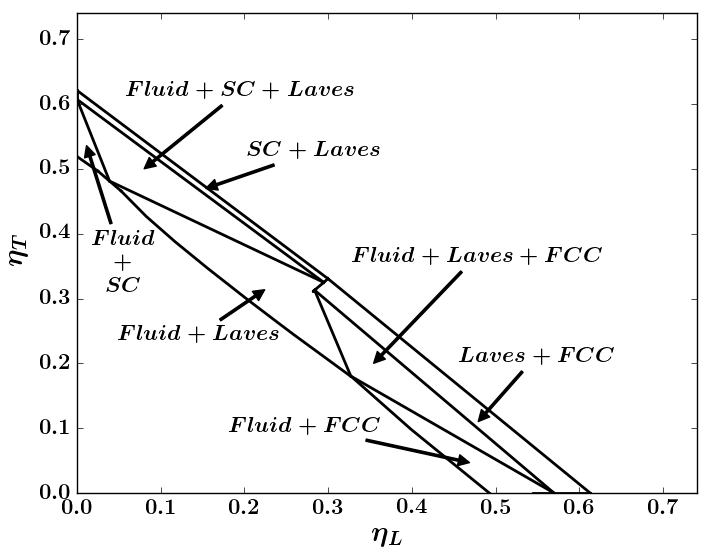
Despite the progress in the fabrication of colloidal building blocks, we are unaware, to the best of our knowledge, of experimental realisations of the proposed binary mixture. In order to facilitate the comparison with experimental results we additionally convert the phase diagram to the packing fraction of tetramers $\eta_{T}$ – packing fraction of spheres $\eta_{S}$ representation, the result being shown in Fig. 8. The triple points we found in Fig. 6 – Fluid + SC + Laves, Fluid + Laves + FCC – transform to triangular areas in this representation. In between the triple points we find the coexistence region between fluid phase and Laves structure, which could be probed experimentally. Note that the triple point SC + Laves + FCC is outside the scanned pressure range and for this reason does not appear in Fig. 8. Finally, we also calculate the phase diagram in the chemical potential of the spheres $\mu_{L}$ – chemical potential of the tetramer $\mu_{T}$ representation. While this diagram is not suitable for comparison with experiments, it is instead crucial in order to theoretically address the role of gravity on the presented bulk results, as accomplished in the next section.

References

- [1] M. N. Rosenbluth and A. W. Rosenbluth, The Journal of Chemical Physics 22, 881 (1954).
- [2] W. W. Wood and J. D. Jacobson, The Journal of Chemical Physics 27, 1207 (1957).
- [3] B. J. Alder and T. E. Wainwright, The Journal of Chemical Physics 27, 1208 (1957).
- [4] P. N. Pusey and W. van Megen, Nature 320, 340 (1986).
- [5] V. J. Anderson and H. N. W. Lekkerkerker, Nature 416, 811 (2002).
- [6] P. J. Lu and D. A. Weitz, Annual Review of Condensed Matter Physics 4, 217 (2013).
- [7] B. Li, D. Zhou, and Y. Han, Nature Reviews Materials 1, 15011 (2016).
- [8] A. Stein, B. E. Wilson, and S. G. Rudisill, Chem. Soc. Rev. 42, 2763 (2013).
- [9] G. von Freymann, V. Kitaev, B. V. Lotsch, and G. A. Ozin, Chem. Soc. Rev. 42, 2528 (2013).
- [10] H. Cong, B. Yu, J. Tang, Z. Li, and X. Liu, Chem. Soc. Rev. 42, 7774 (2013).
- [11] J. Xu and Z. Guo, Journal of Colloid and Interface Science 406, 1 (2013).
- [12] J. Zhang, Z. Sun, and B. Yang, Current Opinion in Colloid & Interface Science 14, 103 (2009).
- [13] C. López, Advanced Materials 15, 1679 (2003).
- [14] J. F. Galisteo-López, M. Ibisate, R. Sapienza, L. S. Froufe-Pérez, Á. Blanco, and C. López, Advanced Materials 23, 30 (2011).
- [15] J. Ge and Y. Yin, Angewandte Chemie International Edition 50, 1492 (2011).
- [16] S. Furumi, H. Fudouzi, and T. Sawada, Laser & Photonics Reviews 4, 205 (2010).
- [17] D. K. Cullen, Y. Xu, D. V. Reneer, K. D. Browne, J. W. Geddes, S. Yang, and D. H. Smith, NeuroImage 54, S37 (2011).
- [18] H. S. Lee, T. S. Shim, H. Hwang, S.-M. Yang, and S.-H. Kim, Chemistry of Materials 25, 2684 (2013).
- [19] I. B. Burgess, L. Mishchenko, B. D. Hatton, M. Kolle, M. Lončar, and J. Aizenberg, Journal of the American Chemical Society 133, 12430 (2011).
- [20] V. P. Bykov, Soviet Journal of Quantum Electronics 4, 861 (1975).
- [21] E. Yablonovitch, Phys. Rev. Lett. 58, 2059 (1987).
- [22] E. Yablonovitch, T. J. Gmitter, and K. M. Leung, Phys. Rev. Lett. 67, 2295 (1991).
- [23] E. Yablonovitch, J. Opt. Soc. Am. B 10, 283 (1993).
- [24] K. M. Ho, C. T. Chan, and C. M. Soukoulis, Phys. Rev. Lett. 65, 3152 (1990).
- [25] K. Ho, C. Chan, C. Soukoulis, R. Biswas, and M. Sigalas, Solid State Communications 89, 413 (1994).
- [26] H. Sözüer and J. P. Dowling, Journal of Modern Optics 41, 231 (1994).
- [27] H. S. Sözüer and J. W. Haus, J. Opt. Soc. Am. B 10, 296 (1993).
- [28] H. S. Sözüer, J. W. Haus, and R. Inguva, Phys. Rev. B 45, 13962 (1992).
- [29] S. G. Johnson and J. D. Joannopoulos, Applied Physics Letters 77, 3490 (2000).
- [30] S.-Y. Lin, J. Fleming, D. Hetherington, B. Smith, R. Biswas, K. Ho, M. Sigalas, W. Zubrzycki, S. Kurtz, and J. Bur, Nature 394, 251 (1998).
- [31] J. G. Fleming and S.-Y. Lin, Opt. Lett. 24, 49 (1999).
- [32] J. E. G. J. Wijnhoven and W. L. Vos, Science 281, 802 (1998).
- [33] R. C. Schroden, M. Al-Daous, C. F. Blanford, and A. Stein, Chemistry of Materials 14, 3305 (2002).
- [34] Y. A. Vlasov, X.-Z. Bo, J. C. Sturm, and D. J. Norris, Nature 414, 289 (2001).
- [35] M. Qi, E. Lidorikis, P. T. Rakich, S. G. Johnson, J. D. Joannopoulos, E. P. Ippen, and H. I. Smith, Nature 429, 538 (2004).
- [36] M. Maldovan and E. L. Thomas, Nat Mater 3, 593 (2004).
- [37] E. C. M. Vermolen, J. H. J. Thijssen, A. Moroz, M. Megens, and A. van Blaaderen, Opt. Express 17, 6952 (2009).
- [38] V. N. Manoharan, M. T. Elsesser, and D. J. Pine, Science 301, 483 (2003).
- [39] C. Young-Sang, Y. Gi-Ra, K. Shin-Hyun, D. J. Pine, and Y. Seung-Man, Chemistry of Materials 17, 5006 (2005).
- [40] D. J. Kraft, J. Groenewold, and W. K. Kegel, Soft Matter 5, 3823 (2009).
- [41] C. Liddell and C. Summers, Advanced Materials 15, 1715 (2003).
- [42] S.-M. Yang, S.-H. Kim, J.-M. Lim, and G.-R. Yi, J. Mater. Chem. 18, 2177 (2008).
- [43] Y. Lu, Y. Yin, and Y. Xia, Advanced Materials 13, 415 (2001).
- [44] J.-T. Wang, J. Wang, and J.-J. Han, Small 7, 1728 (2011).
- [45] S. Sacanna and D. J. Pine, Current Opinion in Colloid & Interface Science 16, 96 (2011).
- [46] Y. Yin and Y. Xia, Advanced Materials 13, 267 (2001).
- [47] Y. Xia, Y. Yin, Y. Lu, and J. McLellan, Advanced Functional Materials 13, 907 (2003).
- [48] L.-Y. Chu, A. Utada, R. Shah, J.-W. Kim, and D. Weitz, Angewandte Chemie International Edition 46, 8970 (2007).
- [49] E. Duguet, A. Desert, A. Perro, and S. Ravaine, Chem. Soc. Rev. 40, 941 (2011).
- [50] T. T. Ngo, C. M. Liddell, M. Ghebrebrhan, and J. D. Joannopoulos, Applied Physics Letters 88, 241920 (2006).
- [51] A.-P. Hynninen, J. H. Thijssen, E. C. Vermolen, M. Dijkstra, and A. Van Blaaderen, Nature Materials 6, 202 (2007).
- [52] A.-P. Hynninen, L. Filion, and M. Dijkstra, The Journal of Chemical Physics 131, 064902 (2009).
- [53] J. H. Zhu, C. T. Liu, L. M. Pike, and P. K. Liaw, Metallurgical and Materials Transactions A 30, 1449 (1999).
- [54] A. R. Edwards, Metallurgical Transactions 3, 1365 (1972).
- [55] M. Parrinello and A. Rahman, Phys. Rev. Lett. 45, 1196 (1980).
- [56] L. Filion, M. Marechal, B. van Oorschot, D. Pelt, F. Smallenburg, and M. Dijkstra, Phys. Rev. Lett. 103, 188302 (2009).
- [57] M. Kowalik, K. Tretiakov, and K. Wojciechowski, Computational Methods in Science and Technology 16, 141 (2010).
- [58] D. Frenkel and B. Smit, Understanding Molecular Simulation: From Algorithms to Applications (Computational Science), 2nd ed. (Academic Press, 2001).
- [59] D. Frenkel and A. J. C. Ladd, The Journal of Chemical Physics 81, 3188 (1984).
- [60] M. Marechal and M. Dijkstra, Phys. Rev. E 77, 061405 (2008).
- [61] C. Vega, E. Sanz, J. L. F. Abascal, and E. G. Noya, Journal of Physics: Condensed Matter 20, 153101 (2008).
- [62] D. de las Heras and M. Schmidt, Journal of Physics: Condensed Matter 27, 194115 (2015).
- [63] J. C. Williams, Powder technology 15, 245 (1976).
- [64] A. Rosato, K. J. Strandburg, F. Prinz, and R. H. Swendsen, Phys. Rev. Lett. 58, 1038 (1987).
- [65] A. Esztermann and H. Löwen, Europhys. Lett. 68, 120 (2004).
- [66] M. N. van der Linden, Long-range repulsive charged colloids in and out of equilibrium, Ph.D. thesis, Utrecht University (2013).
- [67] D. de las Heras, N. Doshi, T. Cosgrove, J. Phipps, D. I. Gittins, J. S. van Duijneveldt, and M. Schmidt, Scientific Reports 2, 789 (2012).