Interplay of Coulomb interaction and spin-orbit coupling

We consider electrons that move between $t_{2{\rm g}}$ orbitals $b$ and $b^{\prime}$ on sites $i$ and $j$ of our simple-cubic lattice with $L$ sites. In second quantization the single-particle Hamiltonian reads

where we introduce the combined spin-orbital index

The crystal-field energies are set to zero, $t_{i,i}^{\sigma,\sigma^{\prime}}=0$.

We use the standard parameterization for the hopping amplitudes in (2) with some generic Slater-Koster parameters [19]

for the electron transfers up to 3rd nearest neighbors. By including hoppings beyond the nearest neighbors we make sure that there are no artificial features in our band structure, such as nesting vectors or particle-hole symmetry. In transition metal compounds, the value of $t$ is of the order of $1\,$eV. In our pure model study in this work, we will simply set $t=1$ as our energy unit.

The single-particle Hamiltonian (2) can be readily diagonalized in momentum space,

with the bare dispersion

and ${\bm{k}}$ from the first Brillouin zone. The remaining task is the diagonalization of the $6\times 6$ matrix $\varepsilon_{{\bm{k}};\sigma,\sigma^{\prime}}$ for each ${\bm{k}}$ to obtain the (bare) band structure. For non-interacting electrons, all energy levels up to the Fermi energy $E_{\rm F}$ are filled in the ground state. The corresponding density of states at the Fermi-energy $E_{\rm F}$ is shown in Fig. 1 as a function of both $E_{\rm F}$ and of the average orbital occupation $0\leq n_{\sigma}\leq 1$. The total bandwidth is $W\approx 3.4$.

Apparently, the Hamiltonian for the kinetic energy is not particle-hole symmetric, as can be seen from the density of states at the Fermi energy. Fig. 1 clearly shows that ${\rm DOS}(n_{\sigma})\neq{\rm DOS}(1-n_{\sigma})$. To study the influence of the spin-orbit coupling, we shall later investigate a particle-hole symmetric kinetic energy. For this case, we use the somewhat artificial Slater-Koster parameters for electron transfers between nearest neighbors only,

which lead to a symmetric density of states of bandwidth $W^{\prime}=2$.

In our ferromagnetic calculations we focus on the filling $n_{\sigma}\approx 0.4$ where the (paramagnetic) density of states has a maximum at the Fermi energy. At such a maximum we can expect a stronger tendency towards ferromagnetic order according to the Stoner criterion. [20]

The Coulomb and spin-orbit interaction are assumed to be purely local,

The local Coulomb interaction for a model with three degenerate $t_{2{\rm g}}$ orbitals reads [21]

where we use the convention $\bar{\uparrow}=\;\downarrow$, $\bar{\downarrow}=\;\uparrow$, and $\hat{n}_{i,b,s}=\hat{c}^{\dagger}_{i,b,s}\hat{c}^{\phantom{\dagger}}_{i,b,s}$ counts the electrons with spin $s$ in orbital $b$ on site $i$. Note that for $t_{2{\rm g}}$-orbitals the three parameters in (11) are not independent because they obey the symmetry relation $U^{\prime}=U-2J$. [21]

For the SOC we use

When we work with the following order for our local basis $|\sigma\rangle$,

the six-dimensional SOC matrix $\tilde{\epsilon}^{\rm so}$ in (12) has the well-known form

with the standard two-dimensional Pauli matrices $\tilde{\sigma}_{1}$, $\tilde{\sigma}_{2}$, $\tilde{\sigma}_{3}$, and the SOC constant $\zeta$.

The local Hamiltonian

in the $64$-dimensional local Hilbert space is readily diagonalized,

For parameter values that are typical for transition metals, $\zeta/J=0.2\ldots 1.0$ and $J/U=0.2$, the atomic spectrum has a generic form. In table 1 we list the degenerate eigenspaces of $\hat{H}_{i;{\rm loc}}$, ordered by increasing energy for given particle number $0\leq n_{\rm loc}\leq 6$. We give the degeneracy $g$ of each level, its total spin $s$, orbital moment $l$, and total ‘angular momentum’ $j$.

Since the rotational symmetry is broken in our cubic environment, the quantum numbers $l$ and $j$ do, in fact, not label eigenstates of the total ‘angular momentum’ operator. It is well known, however, that in the $t_{2\rm{g}}$ sub-space we have

for the vector $\tilde{{\bm{l}}}$ of the three matrices

Hence, the orbital moment behaves like that of $l=1$ states (‘T-P equivalence’), [21] because $\langle\hat{{\bm{l}}}^{2}\rangle=1(1+1)=2$. To be more precise, one finds

where on the r.h.s. we introduced the representation of the orbital momentum for ($l=1$) $p$-orbitals. Due to the T-P equivalence we can label the multiplet states $|\Gamma\rangle$ by a quantum number $j$ that formally corresponds to a total angular momentum of $l=1$ orbitals. Table 1 shows that Hund’s rules are still valid for the ground states of all particle numbers if we make the replacement $l\to-l$ in Hund’s third rule, as a consequence of eq. (30). In particular, as seen from table 1, the local spectrum is not particle-hole symmetric. As we will show in Sect. III.1.1, the particle-hole asymmetry induced by the SOC is visible in our itinerant three-band lattice model even when we work with a symmetric density of states.

For the variational investigation of the Hamiltonian (1) we use the Gutzwiller wave functions

where $|\Psi_{0}\rangle$ is a normalized single-particle product state (Slater determinant) and the local Gutzwiller correlator is defined as

Here, we introduce the matrix $\tilde{\lambda}_{i}$ of (complex) variational parameters $\lambda_{i;\Gamma,\Gamma^{\prime}}$ which allows us to optimize the occupation and the form of the eigenstates $|\Gamma_{\rm d}\rangle_{i}$ of $\hat{P}_{i}$.

We assume that the matrix $\tilde{\lambda}_{i}$ is Hermitian which ensures that the eigenstates $|\Gamma_{\rm d}\rangle_{i}$ exist and form a basis of the local Hilbert space. Without SOC it is usually a sensible approximation to work with a diagonal (and hence real) matrix $\tilde{\lambda}_{i}$. For a finite SOC, however, it is essential to include at least some non-diagonal elements in $\tilde{\lambda}_{i}$. In this work, we will take into account all non-diagonal parameters in $\lambda_{i;\Gamma,\Gamma^{\prime}}$ with states $|\Gamma\rangle_{i}$ and $|\Gamma^{\prime}\rangle_{i}$ that have the same particle number.

The evaluation of expectations values with respect to the wave function (31) poses a difficult many-particle problem that cannot be solved in general. As shown in Refs. [11, 22], it is possible to derive analytical expressions for the variational ground-state energy in the limit of infinite spatial dimensions ($D\to\infty$). An application of this energy functional to finite-dimensional systems is usually termed ‘Gutzwiller approximation’. It will also be used in this work. One should keep in mind, however, that the Gutzwiller approximation has its limitations, and the study of some phenomena requires an evaluation of expectation values in finite dimensions. [23, 24]

Since the energy functional of the Gutzwiller approximation has been derived in detail in previous work, we will only summarize the main results in this section. In the following we are only interested in systems and wave functions that are translationally invariant. Hence, we shall drop lattice-site indices whenever this does not lead to ambiguities.

As shown in Refs. [11, 22] it is most convenient for the evaluation of Gutzwiller wave functions in infinite spatial dimensions to impose the following (local) constraints

for the local correlation operators $\hat{P}\equiv\hat{P}_{i}$. Here, we introduce the local density matrix $\tilde{C}\equiv\tilde{C}_{i}$ with the elements

Note that the order of indices in (35) has been chosen deliberately because it slightly simplifies the analytical results in Sect. II.2.5.

The constraints can be evaluated by means of Wick’s theorem; explicit expressions are given in Appendix A. In systems with a high symmetry, the matrix $\tilde{C}$ is often diagonal, e.g., for $d$ orbitals in a cubic environment. In such a case, one usually has to take into account only the diagonal constraints (34), because the l.h.s. of (34) for $\sigma\neq\sigma^{\prime}$ is automatically zero for all values of $\tilde{\lambda}_{\rm i}$ that are included in the variational Ansatz. Here, the matrix $\tilde{C}$ is non-diagonal in our system with a finite SOC. Even if one introduces a local basis which has a diagonal local density matrix with respect to $\left|\Psi_{0}\right\rangle$, see Appendix A, one still has to take into account some non-diagonal constraints.

Each local operator $\hat{O}_{i}$, e.g., the operator $\hat{H}_{i;{\rm so}}$, can be written as

In infinite dimensions the expectation value of $\hat{O}_{i}$ has the form

where the remaining expectation values

can readily be evaluated using Wicks theorem, see Appendix A.

The expectation value of a hopping operator in infinite dimensions reads ($i\neq j$)

where an analytical expression for the (local) renormalization matrix $q_{\sigma}^{\sigma^{\prime}}$ is also given in Appendix A. Note that the matrix $q_{\sigma}^{\sigma^{\prime}}$ is, in general, neither real nor Hermitian. Any symmetries among its elements are caused by those of the orbital basis states $|\sigma\rangle$ and the form of the Gutzwiller wave function. For example, if we have no SOC and no magnetic or orbital order in our degenerate three-band system, the renormalization matrix has the simple form $q_{\sigma}^{\sigma^{\prime}}=\delta_{\sigma,\sigma^{\prime}}\sqrt{q}$ with only one renormalization factor for all orbitals.

In a translationally invariant system, the expectation values that we introduced in the previous section lead to the following variational energy functional (per lattice site)

Here, we introduce the tensor

with the bare dispersion $\varepsilon_{{\bm{k}};\sigma,\sigma^{\prime}}$ from eq. (8).

The energy (41) is a function of $\lambda_{\Gamma,\Gamma^{\prime}}$ and $\left|\Psi_{0}\right\rangle$ where $\left|\Psi_{0}\right\rangle$ enters (41), (42) solely through the (non-interacting) density matrix $\tilde{\rho}$ with the elements

Note that the non-local elements of $\tilde{\rho}$ ($i\neq j$) determine the tensor (42) while its local elements

as introduced in eq. (35), enter the elements $q_{\sigma}^{\sigma^{\prime}}$ of the renormalization matrix, the expectation value (39), and the constraints (33), (34).

The energy

has to be minimized with respect to the variational parameters $\lambda_{\Gamma,\Gamma^{\prime}}$ and the density matrices $\tilde{\rho}$ and $\tilde{C}$ obeying the constraints (33), (34), (44), and

This additional constraint ensures that $\tilde{\rho}$ corresponds to a Slater determinant $|\Psi_{0}\rangle$. Note that introducing the local density matrix $\tilde{C}$ as an independent variational object in (45), at the expense of the additional constraint (44), is actually not necessary. Instead one could consider the energy solely as a function of $\tilde{\lambda},\tilde{\rho}$. Our form of the energy functional, however, will turn out to be slightly more convenient because, in the Gutzwiller approximation, $\tilde{\rho}$ enters the energy in a non-linear way only through its local elements.

We introduce the real and the imaginary parts of the variational parameters

Due to the Hermiticity of $\tilde{\lambda}$ we have

which leads to a number $n_{v}$ of independent (and real) variational parameters $\lambda_{\Gamma^{\prime},\Gamma}^{({\rm r/i})}$. They will be considered as the components $v_{z}$ of the $n_{v}$-dimensional vector

The (in general) complex constraints (33), (34) are not all independent, e.g., because of the Hermiticity of $\tilde{g}^{\rm c}$. We denote the set of all independent real and imaginary parts of (33), (34) by the $n_{c}$ real constraints

The constraints (44), (46), and (51) are implemented via Lagrange parameters $\eta_{\sigma,\sigma^{\prime}}$, $\Omega_{(i\sigma),(j\sigma^{\prime})}$, and $\Lambda_{l}$. This leads to the Lagrange functional

which provides the basis of our minimization.

As shown, e.g., in Ref. [25], the minimization of (52) with respect to $\tilde{\rho}$ leads to the effective single-particle Hamiltonian

with the renormalized hopping parameters

The optimal Slater determinant $\left|\Psi_{0}\right\rangle$ is the ground state of $\hat{H}^{\rm eff}_{0}$,

From the minimization of (52) with respect to $\tilde{C}$ we obtain an equation for $\eta_{\sigma,\sigma^{\prime}}$ in (53),

Finally, the minimization with respect to ${\bm{v}}$

determines the Lagrange parameters $\Lambda_{l}$ and the optimal value of ${\bm{v}}$. Equations (53)–(57) need to be solved self-consistently. In Appendix B we explain in more detail how we solve this problem numerically. Note that our minimization algorithm does not require the constraints $g_{l}({\bm{v}},\tilde{C})$ to be independent. This is a major advantage over the method that we had proposed in the earlier work [25].

Without any breaking of spin or orbital symmetries, the minimization of the Gutzwiller energy functional leads to effective on-site energies (56) that have the same form as the SOC (14) but with the coupling constant $\zeta$ replaced by $\zeta^{\rm eff}$. This change from the bare to an effective coupling constant also changes the quasi-particle dispersion of $\hat{H}_{0}^{\rm eff}$. Therefore, the energy splittings at certain high-symmetry points as seen in ARPES experiments are a measure for the effective, not the bare spin-orbit coupling. Note that extracting the quasi-particle dispersion from our Gutzwiller approach relies on a Fermi-liquid interpretation. [26] However, all changes of the effective single-particle Hamiltonian, e.g., energy shifts, are related to changes of certain ground-state expectation values. Since the latter are variationally controlled, it is very likely that the exact single-particle spectrum reflects the same trends.

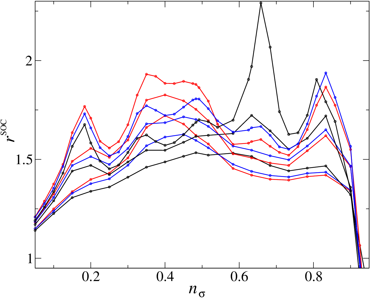
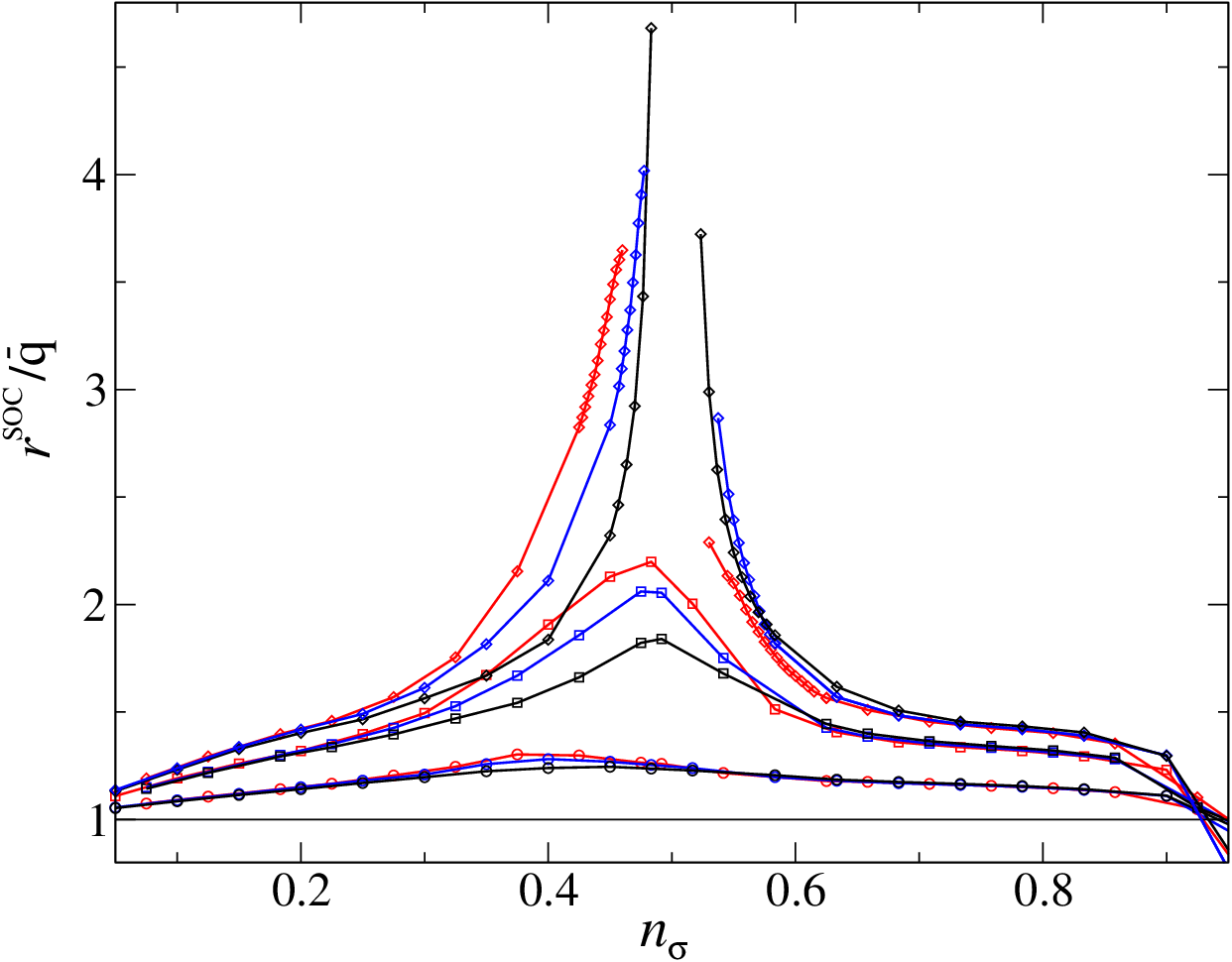
In Fig. 2 we show the renormalization of $\zeta$,

as a function of the orbital occupation $n_{\sigma}$ for the three bare values $\zeta=0.05,0.1,0.2$ and interaction parameters $U=2,3,4$ and $J=0$. Apparently, the effective spin-orbit coupling increases as a function of $U$, apart from a small region of an almost filled shell where $\zeta^{\rm eff}(U)<\zeta$. For $U=4$, which is approximately equal to the band width, the spin-orbit couping can be renormalized by a factor two or more, $r^{\rm SOC}(U=4,n_{\sigma}=2/3,\zeta=0.2)\approx 2.3$. This substantial increase is clearly visible in the quasi-particle band structure, see Fig. 3, where we show the bare ($U=J=0$) and renormalized band structures ($U=4,J/U=0.2$) for $n_{\sigma}=2/3$ and $\zeta=0.2$. For example, the splitting of the bands at the $\Gamma$-point and the R-point is noticeably enhanced in presence of the Coulomb interaction.

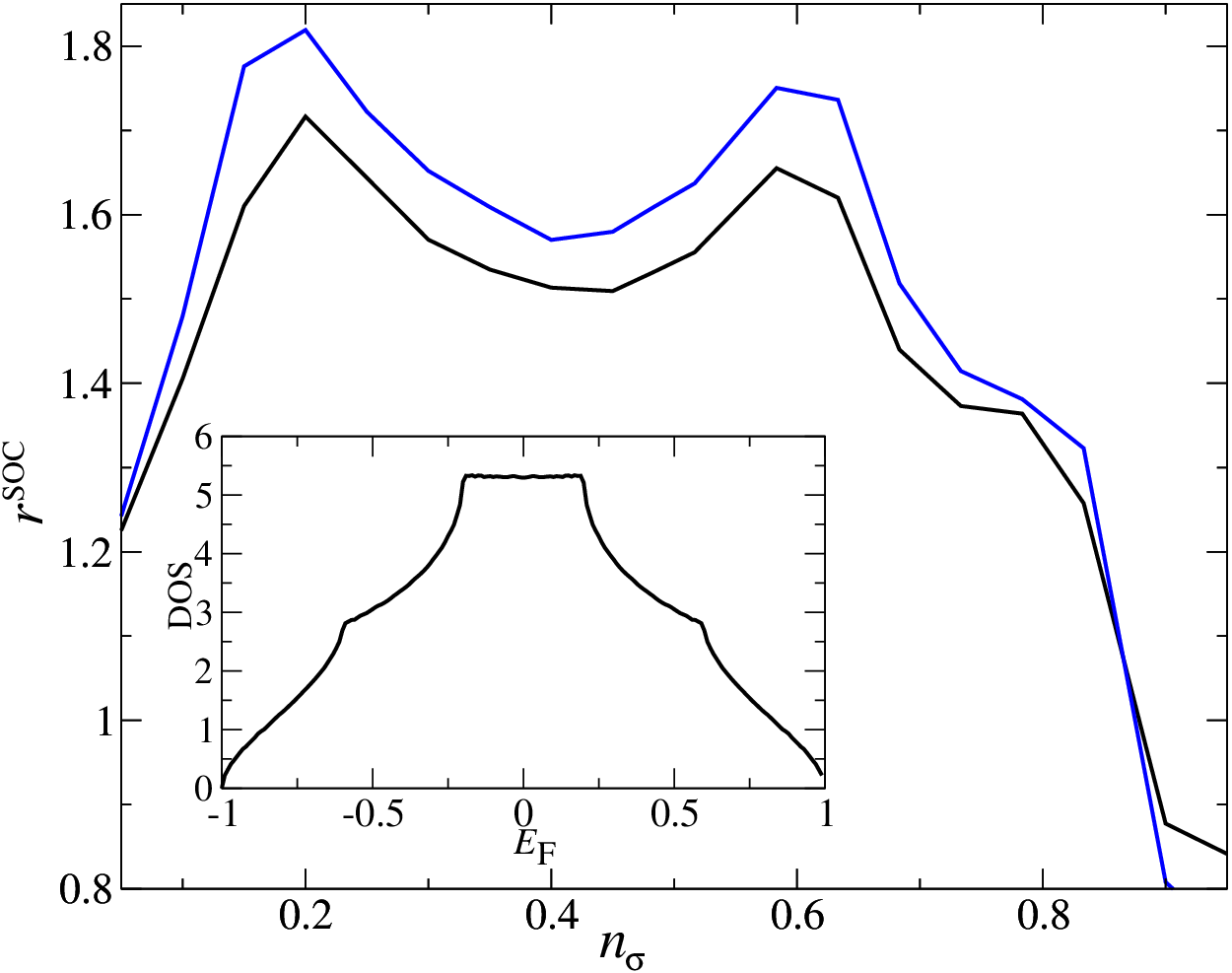
The renormalization $r^{\rm SOC}$ is not monotonous as a function of the bare coupling $\zeta$. Moreover, it is not particle-hole symmetric, i.e., it is not invariant under the transformation $n_{\sigma}\to 1-n_{\sigma}$. This is only partly caused by the particle-hole asymmetry of the bare density of states in Fig. 1. As discussed already in Sect. II.1.2, the SOC inherently breaks the particle-hole symmetry. To illustrate this point, we show the results for a symmetric density of states that results from the nearest-neighbor electron transfers (9), displayed in the inset of Fig. 4. As seen from the figure, the SOC alone induces a particle-hole asymmetry in the renormalization of the effective spin-orbit coupling. We not in passing, that band structures with a fairly similar density of states may, nevertheless, display a very different $n_{\sigma}$ dependence of $r^{\rm SOC}$. Apparently, the full momentum dependence of the band structure determines the details of the $r^{\rm SOC}$-curves.

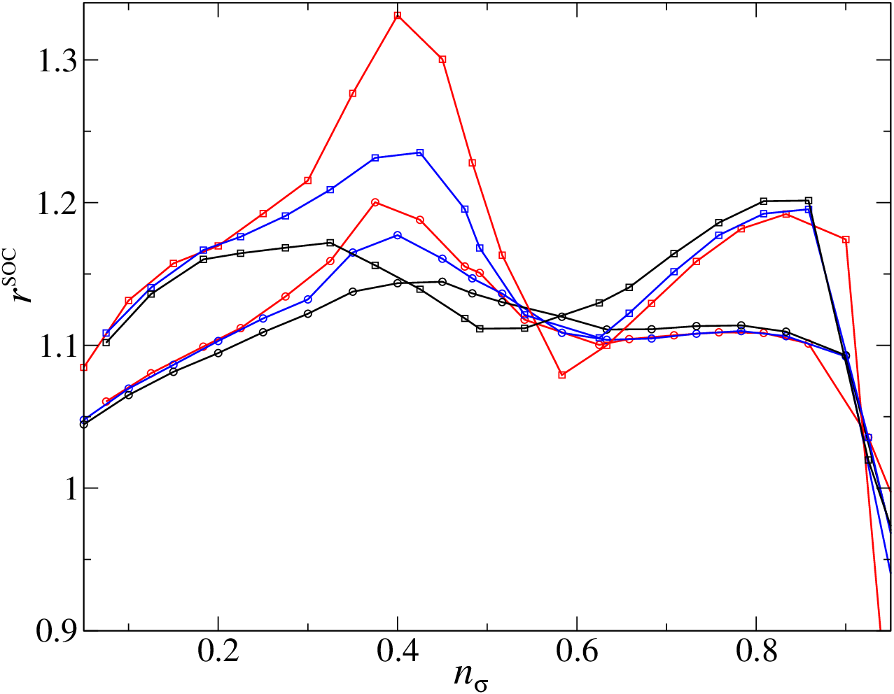
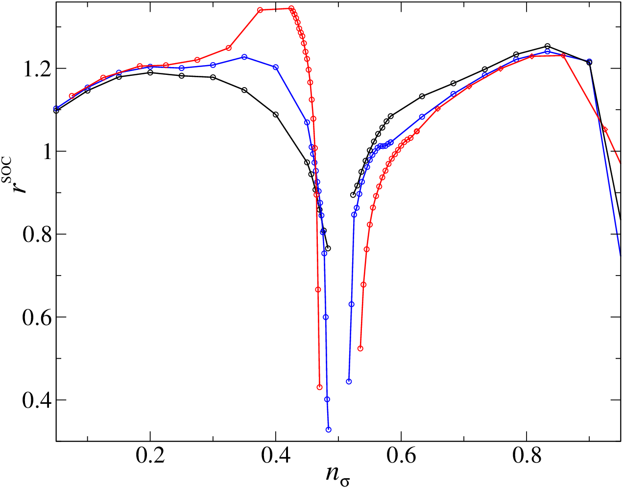
For finite values of the exchange interaction $J$, the effective coupling constants are smaller than for $J=0$, in general. This can be seen in Figs. 5 and 6 where we show the renormalization for $J/U=0.2$, and $U=1,2$ (Fig. 5), $U=2.5$ (Fig. 6). Note that for $U=U_{\rm c}\lesssim 2.5$ there appears a Brinkmann-Rice type of insulating phase[27] at half filling where the renormalization matrix $\tilde{q}$ is zero. Therefore we could perform our calculations shown in Fig. 6 only away from half filling.

The dependence of the renormalization on the band-filling $n_{\sigma}$ appears to be even more complicated for finite $J$, in particular in the region around half filling. One must keep in mind, however, that there is a ‘trivial’ contribution to the renormalization of $\zeta$ which simply stems from the band-width renormalization induced by the renormalization matrix $q^{\sigma^{\prime}}_{\sigma}$. To understand this effect, we consider, for the sake of argument, a renormalization matrix of the simplest form $q^{\sigma^{\prime}}_{\sigma}=\delta_{\sigma,\sigma^{\prime}}\sqrt{q}$. In that case, the effective hopping parameters in (53) are given by $\bar{t}^{\sigma,\sigma^{\prime}}_{i,j}=qt^{\sigma,\sigma^{\prime}}_{i,j}$. Hence, in order to obtain the same expectation values of $\left|\Psi_{0}\right\rangle$ as in the non-interacting limit, we must introduce a scaling $\zeta\to q\zeta<\zeta$. The effect of the enhancement of $\zeta^{\rm eff}$ is therefore amplified by the renormalization of the hopping parameters.

For a more quantitative analysis, we define an average value $\bar{q}$ of the bandwidth renormalization through

i.e., $\bar{q}$ quantifies the reduction of the average kinetic energy in presence of the Coulomb interaction. The relative SOC-renormalization is then plotted in Fig. 7 for the same parameters as in Fig. 5. It shows that the non-trivial renormalization is, in fact, largest in the region around half filling. Moreover, it is actually fairly independent of the bare SOC, a feature that cannot be seen in the original representation of the data in Fig. 5.

In the introduction we raised the question if, and to what extent, Hund’s rules are still discernible in a solid. To clarify this issue, we define the three ‘quantum numbers’ $s,l,j$ via the local expectation values

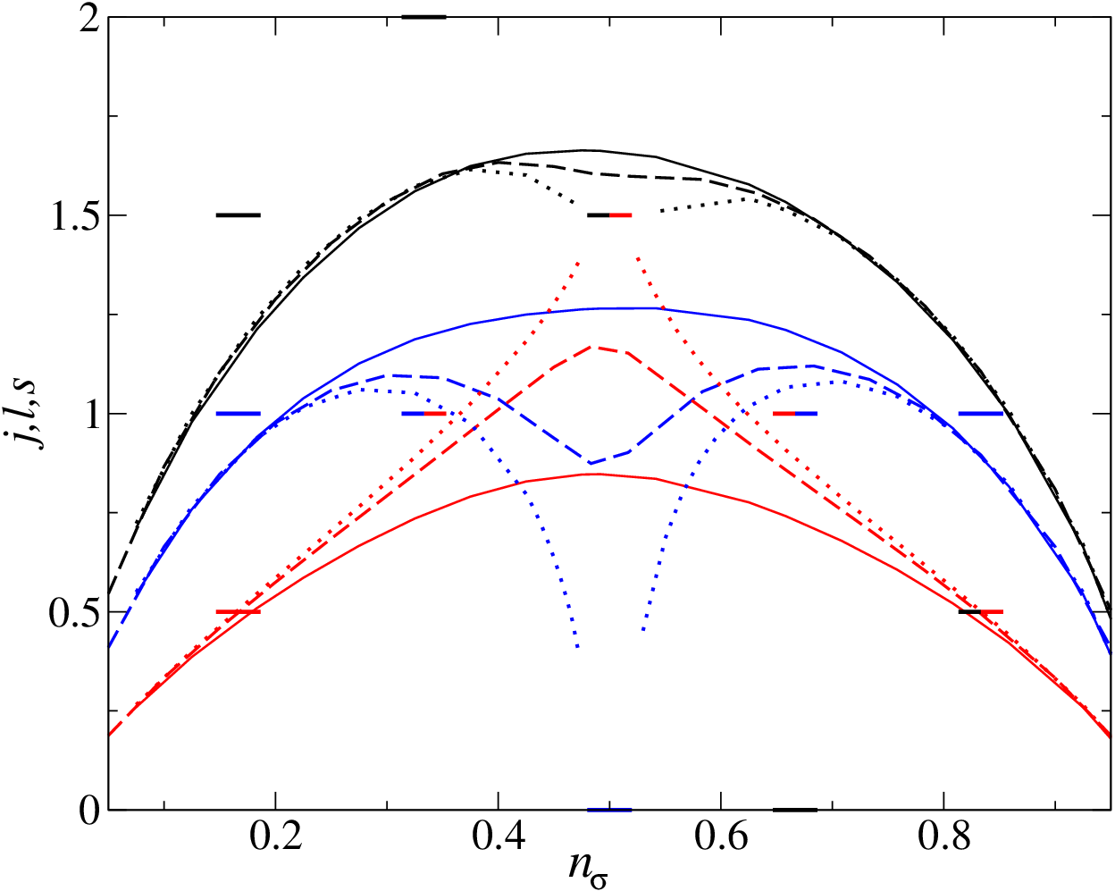
Figure 8 shows these three numbers for $\zeta=0.05$, $J/U=0.2$ and $U=1,2,2.5$. The bars give the values in the atomic limit, as extracted from the ground states in table 1. As expected, all quantum numbers move towards their atomic values when we increase the Coulomb interaction parameters. This is best visible near half-filling when the system is close to the metal-insulator transition that appears at half filling.

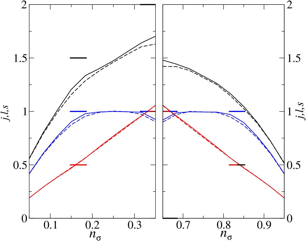
As shown in previous work,[28, 11] this transition is of first-order where in the Gutzwiller insulating state all atoms are in their ground state. This means that at $U_{c}$ all three quantum numbers will jump to their atomic values at half filling. For all other (integer) fillings, the system is still rather itinerant and some of the quantum numbers, in particular $j$, deviate significantly from their atomic values. This is best visible at a filling of $n_{\sigma}=2/3$ where the value of $j$ is far off its atomic value $j_{\rm atomic}=0$. The results change only slightly when we increase the values of $U$ (and $J$) as can be seen from Fig. 9 where we display $j$, $l$, and $s$ for larger values of $U$ away from half filling.

The difference between the behavior close to half filling and the other integer fillings can be understood from the atomic spectra. The high-spin ground state at half filling is only slightly changed by a small SOC and, most importantly, its degeneracy is not lifted. Hence, the energy difference between the Hund’s-rule ground state and the first excited state is of the order of $J$. In contrast, at all other integer fillings, the ground states are created by a splitting of the (degenerate) ground states at $\zeta=0$, caused by the SOC. Therefore, the energy difference between the Hund’s-rule ground state and the first excited states is much smaller away from half filling. As a consequence, it is energetically not favorable to lose a lot of kinetic energy by only occupying the Hund’s-rule ground state. Unlike in the half-filled case, the Hund’s-rule ground state does not dominate the quantum numbers in the metallic phase at or around other integer fillings. As seen from Figs. 8 and 9, only Hund’s first rule is seen to be obeyed in strongly correlated paramagnetic metals close to integer fillings.

In Fig. 10 we display the total spin $S\equiv|\langle\hat{{\bm{S}}}_{i}\rangle|$ for seven different values of $\zeta$ ($0\leq\zeta\leq 0.3)$ as a function of $U$ for $J/U=0.2$. As seen from the figure, the SOC destabilizes the ferromagnetic order, i.e., the value $U_{c}$ for noticeable ferromagnetic order ($S>0.1$) substantially increases as a function of $\zeta$. Concomitantly, the ordered magnetic moment $m=2S$ strongly depends on the SOC as long as the magnetic order is weak, $S<1/2$. The SOC becomes a small perturbation only in the saturation region, $S>1$.

The SOC not only reduces the ordered spin moment, it also induces an orbital moment, i.e., $L\equiv|\langle\hat{{\bm{L}}}_{i}\rangle|$ is non-zero. This is shown in Fig. 11 where we display $L$ for the same parameters as in Fig. 10, apart from $\zeta=0$ where $L=0$. The orbital contribution to the magnetic moment, however, remains rather small, of the order of 10% of the spin moment, especially for values of $\zeta<0.1$ that are realistic for transition metals. Therefore, the gain in orbital moment does not compensate the loss in the ordered spin moment induced by the spin-orbit coupling.

Finally, we take a look at the ‘anisotropy energy’, i.e., the dependence of the energy on the magnetic-moment direction. To this end, we could introduce additional constraints that fix the moment direction during the minimization. However, this would require additional programming work that we prefer to avoid. Therefore, we apply an external magnetic field that allows us to change the magnetic-moment direction. In fact, this is how the anisotropy energy would actually be measured.

Since our field is just a technical tool, we couple it to the spin only, i.e., we add

to the Hamiltonian of our system. Here, ${\bm{e}}_{B}$ is the direction of the magnetic field that we adjust in our calculations. The size of the field amplitude $B$ must be chosen with care to obtain meaningful results. On the one hand, it must be large enough to force the magnetic moment into all directions that we aim to investigate, i.e., in the ground state we must approximately find $\langle{\bm{S}}_{i}\rangle_{\rm G}||{\bm{e}}_{B}$. On the other hand, the variation in the field contribution to the energy must be small compared to the variation of the system’s energy that we actually want to determine. Meeting these criteria becomes difficult, in particular, in the region of small magnetic moments. In all calculations that we are going to present below, we found that a field amplitude of $B=0.002$ leads to meaningful results for the anisotropy energy.

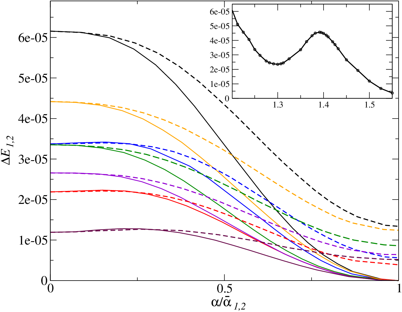
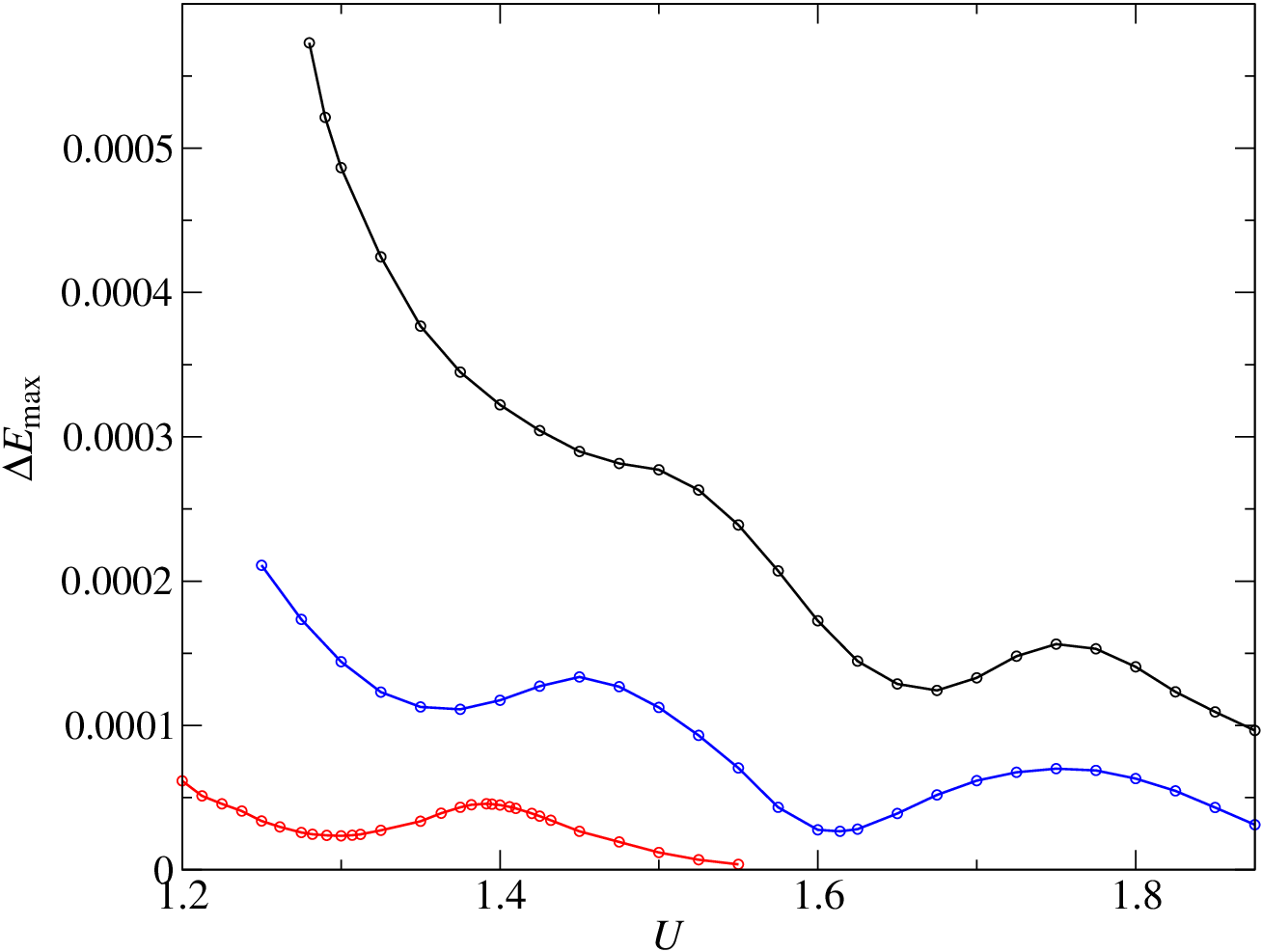
In the following we consider rotations of the magnetic moment from the $(1,0,0)$ direction, (1), into the $(1,1,1)$ direction, and, (2), into the $(1,1,0)$ direction. The corresponding maximal rotation angles are $\bar{\alpha}_{1}=\arccos{(1/\sqrt{3})}$ and $\bar{\alpha}_{2}=\pi/4$, respectively. From our minimization we obtain the two energies $E_{1,2}(\alpha)$ as a function of the angle $\alpha$. Since, as mentioned before, the easy axis always points into the $(1,1,1)$-direction, we define the anisotropy energy as $\Delta E_{i}(\alpha)\equiv E_{i}(\alpha)-E_{1}(\bar{\alpha}_{1})$. This quantity is displayed in Fig. 12 for several values of $U$ (and consequently also different values of the magnetic moment) for $J/U=0.2$ and $\zeta=0.1$. The figure shows that, although the anisotropy energy is quite small, of the order of several ten $\mu$eV per site, our approach is perfectly capable to resolve it. The maximal anisotropy energy $\Delta E_{\rm max}$, i.e., its value for $\alpha=0$ is a non-trivial function of $U$. This can be seen from the inset of Fig. 12 where we display $\Delta E_{\rm max}$.

When we increase the SOC, the anisotropy energies change significantly, see Fig. 13 where we show $\Delta E_{\rm max}$ as a function of $U$ for $\zeta=0.1,0.15,0.2$. The non-monotonic behavior of $\Delta E_{\rm max}$ has its cause in the band structure. For example, the maxima in the red and blue curves and the corresponding structure in the black curve correspond to almost the same magnetization, cf. Fig. 10.

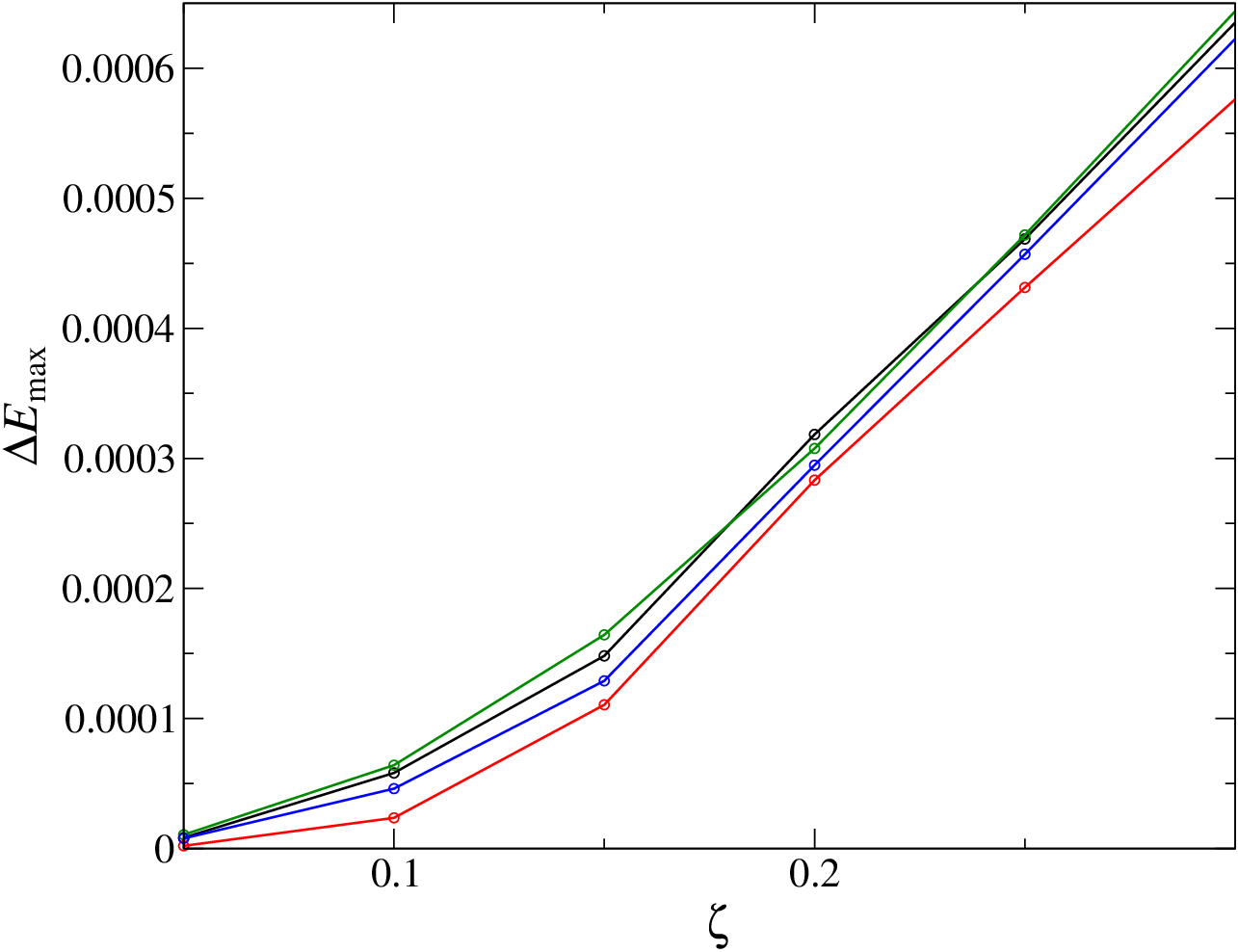
To extract the genuine $\zeta$ dependence of $\Delta E_{\rm max}$, it is best to consider states with the same moment. This is done in Fig. 14 where we display $\Delta E_{\rm max}$ as a function of $\zeta$ for values of $U$ which lead to the same ordered spin moments. These curves reveal that the anisotropy depends very sensitively on $\zeta$ for small values of $\zeta$ whereas it becomes linear for sizable $\zeta$.

References

- [1] F. Hund. Zeitschrift für Physik, 40:742, 1927.
- [2] F. Hund. Zeitschrift für Physik, 42:93, 1927.
- [3] J.-P. Julien, J.-X. Zhu, and R. C. Albers. Phys. Rev. B, 77:195123, 2008.
- [4] L. Du, L. Huang, and X. Dai. Eur. Phys. J. B, 86:94, 2013.
- [5] L. Du, X. Sheng, H. Weng, and X. Dai. Europhys. Lett., 101:27003, 2013.
- [6] A. Farrell and T. Pereg-Barnea. Phys. Rev. B, 89:035112, 2014.
- [7] H. Shinaoka, S. Hoshino, M. Troyer, and P. Werner. Phys. Rev. Lett., 115:156401, 2015.
- [8] G. Zhang, E. Gorelov, E. Sarvestani, and E. Pavarini. Phys. Rev. Lett., 116:106402, 2016.
- [9] Z. Y. Meng, Y. B. Kim, and H.-Y. Kee. Phys. Rev. Lett., 113:177003, 2014.
- [10] A. O. Shorikov and V. I. Anisimov. arxiv:1412.0140.
- [11] J. Bünemann, W. Weber, and F. Gebhard. Phys. Rev. B, 57:6896, 1998.
- [12] W. Metzner and D. Vollhardt. Phys. Rev. Lett., 59:121, 1987.
- [13] F. Gebhard. Phys. Rev. B, 41:9452, 1990.
- [14] K. zu Münster and J. Bünemann. Phys. Rev. B, 2016.
- [15] K. M. Ho, J. Schmalian, and C. Z. Wang. Phys. Rev. B, 77:073101, 2008.
- [16] X. Deng, X. Dai, and Z. Fang. Europhys. Lett., 83:37008, 2008.
- [17] T. Schickling, J. Bünemann, F. Gebhard, and W. Weber. New Journal of Physics, 16:93034, 2014.
- [18] T. Schickling, J. Bünemann, L. Boeri, and F. Gebhard. Phys. Rev. B, 2016.
- [19] J. C. Slater and G. F. Koster. Phys. Rev., 94:1498, 1954.
- [20] E. C. Stoner. Proc. of the Royal Soc. London A, 165:372, 1938.
- [21] S. Sugano, Y. Tanabe, and H. Kamimura. Multiplets of Transition-Metal Ions in Crystals. Pure and Applied Physics 33, Academic Press, New York, 1970.
- [22] J. Bünemann, F. Gebhard, and W. Weber. In A. Narlikar, editor, Frontiers in Magnetic Materials. Springer, Berlin, 2005.
- [23] J. Büneman, T. Schickling, and F. Gebhard. Europhys. Lett., 98:27006, 2012.
- [24] J. Kaczmarczyk, J. Spałek, T. Schickling, and J. Bünemann. Phys. Rev. B, 88:115127, 2013.
- [25] J. Bünemann, F. Gebhard, T. Schickling, and W. Weber. physica status solidi (b), 249:1282, 2012.
- [26] J. Bünemann, F. Gebhard, and R. Thul. Phys. Rev. B, 67:75103, 2003.
- [27] W. F. Brinkman and T. M. Rice. Phys. Rev. B, 2:4302, 1970.
- [28] J. Bünemann and W. Weber. Phys. Rev. B, 55:4011, 1997.
- [29] J. Bünemann, T. Linneweber, and F. Gebhard. physica status solidi, 2016.
- [30] S. Hoshino and P. Werner. Phys. Rev. Lett., 115:247001, 2015.
- [31] M. Fabrizio. Phys. Rev. B, 76:165110, 2007.
- [32] J. Nocedal and S. J. Wright. Numerical Optimization. Springer, New York, 2nd edition, 2006.