Landweber-Kaczmarz method in Banach spaces with inexact inner solvers
Abstract.
In recent years Landweber(-Kaczmarz) method has been proposed for solving nonlinear ill-posed inverse problems in Banach spaces using general convex penalty functions. The implementation of this method involves solving a (nonsmooth) convex minimization problem at each iteration step and the existing theory requires its exact resolution which in general is impossible in practical applications. In this paper we propose a version of Landweber-Kaczmarz method in Banach spaces in which the minimization problem involved in each iteration step is solved inexactly. Based on the -subdifferential calculus we give a convergence analysis of our method. Furthermore, using Nesterov’s strategy, we propose a possible accelerated version of Landweber-Kaczmarz method. Numerical results on computed tomography and parameter identification in partial differential equations are provided to support our theoretical results and to demonstrate our accelerated method.
1. Introduction
Regularization of inverse problems has been considered extensively and significant progress has been made; see [10, 18, 21, 26, 34] and references therein. Due to the demand of capturing special features of the reconstructed objects and the demand of dealing with general noise, regularization in Banach spaces has emerged as a highly active research field and many new regularization methods have been proposed and investigated in recent years; one may refer to [5, 17, 19, 23, 24, 25, 33] and the references therein for recent developments.
Because of its simplicity and relatively small complexity per iteration, Landweber iteration and its Kaczmarz version have received extensive attention in inverse problem community [9, 11, 12, 14, 27]. In recent years, several versions of Landweber iteration has been formulated in Banach spaces, see [5, 20, 22, 31]. When solving ill-posed system of the form
| (1.1) |
consisting of equations, a Kaczmarz version of Landweber iteration in Banach spaces with general uniformly convex penalty functions has been proposed in [22] which cyclically considers each equation in (1.1) in a Gauss-Seidel manner. For these modern versions of Landweber method, each iteration step essentially requires the computation of next iterate from current iterate via
where is a step size, is a duality mapping, denote one of , denotes the Fréchet derivative of , and is a uniformly convex function. Therefore, the implementation of the Landweber(-Kaczmarz) method in Banach spaces requires to solving a minimization problem of the form
| (1.2) |
associated with in each iteration step.
The existing convergence theory on Landweber(-Kaczmarz) method in Banach spaces requires the exact resolution of the minimization problem (1.2). For some special its exact resolution is possible. However, this minimization problem in general can only be solved inexactly by an iterative procedure which may produce an approximate solution satisfying
| (1.3) |
for some small . Furthermore, numerical simulations indicate that solving (1.2) very accurately in every step does not improve the final reconstruction result but wastes a huge amount of computational time. Therefore, it is necessary to formulate a Landweber-Kaczmarz method with inexact inner solver in each iteration step and to develop the corresponding convergence theory. The inequality (1.3) suggests that the -subdifferential calculus might be a useful tool for this purpose.
It is well-known that Landweber iteration admits the slow convergence property ([10]) which restricts its applications to wide range of problems. To expand its applied range, it is necessary to introduce some acceleration strategy to fasten its convergence speed. In this paper we will use the Nesterov’s strategy in optimization ([29]) to propose an accelerated version of Landweber-Kaczmarz method in Banach spaces in which some extrapolation steps are incorporated. We do not have a theory to guarantee its acceleration effect at this moment, however, we will provide numerical simulations to support the fast convergence property.
This paper is organized as follows. In section 2 we will provide some preliminaries on Banach spaces and convex analysis and derive some useful results concerning -subdifferential. In section 3 we propose the Landweber-Kaczmarz method with inexact inner solvers, show that it is well-defined, and prove its convergence and regularization property. We then use Nesterov’s strategy to propose an accelerated version. We also discuss how to produce the inexact solvers for solving the inner minimization problem at each iteration step of Landweber-Kaczmarz method. Finally, we provide numerical simulations to verify the theoretical results and to demonstrate the fast convergence of the accelerated method.
2. Preliminaries
Let be two Banach space whose norm is denoted by . We use to denote its dual spaces. For any and , we write for the duality pairing. Let be another Banach space. By we denote for the space of all bounded linear operators from to . For any we use to denote its adjoint, i.e.
for any and .
For each , the set-valued mapping defined by
is called the duality mapping of with gauge function . When is uniformly smooth in the sense that its modulus of smoothness
satisfies , the duality mapping , for each , is single valued and uniformly continuous on bounded sets.
Given a convex function , we use
to denote its effective domain. It is called proper if . For a proper convex function and , we define for any the set
which is called the -subdifferential of at . Any element in is called an -subgradient of at . When , the -subdifferential of reduces to the subdifferential . It is clear that for some implies . If is lower semi-continuous, then for any , the -subdifferential is always non-empty for any , see [35, Theorem 2.4.4]; however, can be empty in general.
For with , we may introduce
which is called the -Bregman distance induced by at in the direction . It is clear that
When , the -Bregman distance becomes the well-known Bregman distance [7] which will be denoted by . It should be pointed out that -Bregman distance is not a metric distance in general. Nevertheless, as the following result shows, the -Bregman distance can be used to detect information under the norm if is -convex for some in the sense that there is a constant such that
| (2.1) |
for all and , .
Lemma 2.1.
Let be a proper, lower semi-continuous function that is -convex in the sense of (2.1). If for some , then
| (2.2) |
for any .
Proof.
In convex analysis, the Legendre-Fenchel conjugate is an important notion. Given a proper convex function , its Legendre-Fenchel conjugate is defined by
As an immediate consequence of the definition, one can see, for any , that
| (2.3) |
If, in addition, is lower semi-continuous, then ([35, Theorem 2.4.4])
| (2.4) |
For a proper, lower semi-continuous, -convex function, even if it is non-smooth, its Legendre-Fenchel conjugate can have enough regularity as the following result indicates.
Lemma 2.2.
Let be a reflexive Banach space and let be a proper, lower semi-continuous function that is -convex in the sense of (2.1). Then , is Fréchet differentiable, and its gradient satisfies
| (2.5) |
which consequently implies
| (2.6) |
for any , where is the number conjugate to , i.e. .
Proof.
See [35, Theorem 3.5.10 and Corollary 3.5.11]. ∎
Finally we conclude this section by providing a result which show that, when is -convex, then, for any , the distance from to can be controlled in terms of .
Lemma 2.3.
Let ba a reflexive Banach space and let be a proper, lower semi-continuous function that is -convex in the sense of (2.1). If and satisfy for some , then for any there holds
| (2.7) |
and hence
| (2.8) |
3. The method
We consider the system
| (3.1) |
consisting of equations, where, for each , is an operator between two reflexive Banach spaces and . Such systems arise in many practical applications including various tomography problems using multiple exterior measurements.
We will assume that (3.1) has a solution which consequently implies that
In practical applications, instead of we only have noisy data satisfying
| (3.2) |
with a small noise level . How to use to produce an approximate solution of (3.1) is an important question. In [22] we proposed a Landweber iteration of Kaczmarz type which makes use of every equation in (3.1) cyclically. In order to capture the feature of the sought solution, general convex functions have been used in [22] as penalty terms.
We will make the following assumption, where .
Assumption 3.1.
According to Assumption 3.1 (c), we can find a constant such that
| (3.4) |
Moreover
| (3.5) |
for all which shows that is continuous on for each .
The formulation of the Landweber iteration of Kaczmarz type in [22] involves in each iteration step a minimization problem of the form
| (3.6) |
for any . The convergence result developed there requires to solving (3.6) exactly. The exact solution of (3.6) can be found for some special . However, this minimization problem in general can only be solved inexactly by iterative procedures. Furthermore, numerical simulations indicate that solving (3.6) very accurately in every step does not improve the final reconstruction result. Therefore, it is necessary to formulate a Landweber-Kaczmarz method with inexact inner solver in each iteration step and to develop the corresponding convergence theory.
Concerning the inexact resolution of (3.6), we make the following assumption.
Assumption 3.2.
For any given there is a procedure for solving (3.6) such that for any , the element satisfies
| (3.7) |
Moreover, for each , the mapping is continuous.
In subsection 3.5 we will discuss how to produce the inexact procedure by using concrete examples of including the total variation like convex penalty functions.
3.1. The method with noisy data
We are ready to formulate our Landweber-Kaczmarz method with inexact inner solvers. We will take and let denote the duality mapping over with gauge function . Given an integer , we set .
Algorithm 3.1 (Landweber-Kaczmarz method with noisy data).
Let , and be suitably chosen numbers, and let be a sequence of positive numbers satisfying .
- (i)
Pick and such that .
- (ii)
Let and . Let and let be a small number. For we define and
We then update
(3.8) where
(3.9) with
- (iii)
Let be the first integer such that and use as an approximate solution.
In Algorithm 3.1, each is determined by completely without involving , and each is defined by the inexact procedure specified in Assumption 3.2 for solving (3.6) which is independent of , . This splitting character can make the implementation of Algorithm 3.1 efficiently. Furthermore, the definition of implies that
which shows that
| (3.10) |
We will use this fact in the forthcoming convergence analysis.
We first prove the following basic result which shows that Algorithm 3.1 is well-defined.
Lemma 3.1.
Let and be reflexive Banach spaces with being uniformly smooth, let and , satisfy Assumption 3.1, and let be a sequence of positive numbers satisfying
| (3.11) |
Let be a constant such that . If and are chosen such that
| (3.12) |
and if is chosen such that , where
| (3.13) |
then for Algorithm 3.1 there hold
- (i)
for all ;
- (ii)
the method terminates after iteration steps;
- (iii)
Proof.
Let be any solution of (3.1) in . We first show that, if for some , then
| (3.15) |
To see this, we consider
which can be written as
Since , we have from (2.3) that
By the definition of we also have
Therefore
Because is -convex, we may use (2.6) in Lemma 2.2 and the definition of to obtain
| (3.16) |
Since , we may use Lemma 2.3 to derive that
Plugging this estimate into (3.16) and using the definition of it follows that
By writing
we may use the condition , Assumption 3.1 (c), and the properties of to obtain
Therefore
| (3.17) |
By the definition of we can see that
and
Combining the above two estimates with (3.17) we can obtain
| (3.18) |
We next consider the term . We claim that
| (3.19) |
where is the constant defined by (3.13). Indeed, this is trivial when . We only need to consider the case that . If , then
If , we may use the inequality for and to derive that
Thus, by using , we have
We therefore obtain (3.19).
Combining (3.18) and (3.19) we thus have
where is the constant defined by (3.12). Since and , we therefore obtain (3.15).
Now we use an induction argument to show that for all . This is trivial when . Assume that there is some such that for . Thus (3.15) holds for all . By taking in (3.15) and summing it over these gives
In view of Lemma 2.1, (3.3) in Assumption 3.1 and (3.11) we can obtain
This implies that . By virtue of (3.3) and Lemma 2.1 we also have . Therefore , i.e. . Consequently, (3.15) holds for all which gives (3.14) immediately. By summing (3.15) over from to we can obtain
| (3.20) |
3.2. The method with exact data
In order to prove the regularization property of Algorithm 3.1, we first consider its counterpart where the noisy data are replaced by the exact data . That is, we will consider the following algorithm.
Algorithm 3.2 (Landweber-Kaczmarz method with exact data).
Let , , , , and be the same as in Algorithm 3.1. For we define and update
| (3.21) |
where and
| (3.22) |
with
By using the same argument in the proof of Lemma 3.1, we can obtain the following result on Algorithm 3.2.
Lemma 3.2.
Let and be reflexive Banach spaces with being uniformly smooth, let and , satisfy Assumption 3.1, and let be a sequence of positive numbers satisfying (3.11). Let be a constant such that . If is chosen such that
| (3.23) |
and if is chosen such that , where is defined by (3.13), then for Algorithm 3.2 there holds for all , and for any solution of (3.1) in there hold
| (3.24) | ||||
| (3.25) |
In the following we will show that the sequence defined by Algorithm 3.2 converges to a solution of (3.1). We first prove that the sequence is convergent.
Lemma 3.3.
Proof.
Lemma 3.4.
For all there holds
Proof.
Recall . This result follows from Lemma 2.3 immediately. ∎
Lemma 3.5.
Let all the conditions in Lemma 3.2 hold. Then there is a universal constant such that
for all and , where .
Proof.
We consider the case ; the case can be considered similarly. Let . By the triangle inequality and (3.5) we have
By virtue of the Hölder inequality and , we can obtain
| (3.27) |
In view of Lemma 3.4 and (2.5), we have
By the definition of and we have
Thus
Combining this with (3.27) gives
where is a universal constant. This completes the proof. ∎
Corollary 3.1.
Now we are ready to prove the convergence on the sequence defined by Algorithm 3.2.
Theorem 3.6.
Proof.
We first show that has a convergent subsequence. To this end, we consider.
Then and, in view of (3.26), we have as . We may choose a strictly increasing subsequence of integers such that and , for each , is the first integer satisfying
For this it can be seen that
| (3.28) |
Indeed, for any satisfying , we can find such that and thus, by the definition of , we have .
With the above chosen , we set and show that is convergent. To this end, we consider the -Bregman distance for . Let be any solution of (3.1) in . By the definition of -Bregman distance, we have
| (3.29) |
We need to consider the term for . We write
According to the definition of we have
By the Cauchy-Schwarz inequality, the property of and the definition of we obtain
By Assumption 3.1 (c) we have
Combining the above two equations and using the Hölder inequality, we can find a universal constant such that
By using Lemma 3.5 we have
Consequently, it follows from (3.28) that
Therefore
This together with (3.26) implies that
| (3.30) |
Thus, it follows from (3.29), Lemma 3.3 and that
In view of Lemma 2.1 and , we can conclude
i.e. is a Cauchy sequence in . Thus as for some . By using Corollary 3.1 and the continuity of we have for all .
We next show that Since , we must have . By using we can obtain
| (3.31) |
In view of (3.30) and , there is a constant such that
Thus for all . By using the lower semi-continuity of and we obtain from (3.31) that
This implies that . Therefore is a solution of (3.1) in .
Finally we show that the whole sequence converges to . Let
whose existence is guaranteed by Lemma 3.3. By the non-negativity of -Bregman distance, we have . In (3.29) we set and take to derive that
This implies that
for all . In view of (3.30), by taking we obtain . Therefore , that is, . By using Lemma 2.1 and we can obtain . ∎
3.3. Regularization property
We return to Algorithm 3.1 and prove its regularization property. We need the following stability result.
Lemma 3.7.
Let all the conditions in Lemma 3.1 hold. Then for all there hold
Proof.
The result is trivial for . We next assume that the result is true for some and show that and as . We consider two cases.
Case 1: . In this case we have . Therefore
Since , we may use the property of and (3.4) to obtain
By the induction hypothesis and the continuity of , we then have as . By the definition of and the continuity of we have
as .
Case 2: . Since , we have for small . Thus
We claim that as . In fact, if then, by definition, we must have and for small . If then, by the definition of and and the induction hypothesis, we can conclude that as . In any case, we always have as . Consequently, by the induction hypotheses and the continuity of , and , we have and therefore as . By invoking again the continuity of , we obtain as . ∎
Theorem 3.8.
Proof.
By the definition of we have . Since for all , we must have as . Let be the solution of (3.1) in determined in Theorem 3.6. In view of Lemma 2.1 and , it suffices to show that
| (3.32) |
Let be an arbitrary but fixed integer. By virtue of Lemma 3.1 we have
Consequently
By making use of Lemma 3.7 and the lower semi-continuity of we have
Therefore
Since can be arbitrarily large, by taking we can derive from Theorem 3.6 and the condition that
This completes the proof. ∎
3.4. Acceleration
It is well-known that Landweber iteration is a slowly convergent method ([10]). In order to make it applicable in practical applications, acceleration strategies should be incorporated into the method. When an inverse problem is formulated in Hilbert spaces, a family of accelerated Landweber iterations, including the famous -method of Brakhage [2], have been proposed in [3] using the orthogonal polynomials and the spectral theory of self-adjoint operators. The acceleration strategy using orthogonal polynomials is no longer available when an inverse problems is considered in Banach spaces using general convex penalty functions. Instead the sequential subspace optimization strategy has been employed in [16, 32] to accelerate the method.
In recent years Nesterov’s acceleration strategy [29] has received tremendous consideration in optimization community. Consider the unconstrained optimization problem
| (3.33) |
in a Hilbert space with a continuous differentiable function . Nesterov’s strategy speeds up the gradient descent method by using a proper extrapolation point at each iteration step. It takes the form
| (3.34) |
with suitable step sizes , where is a fixed number. This strategy has been extended in various context, even for nonsmooth optimization problems, see [2, 3, 8].
Due to the simplicity of Nesterov’s strategy, it is natural to consider its use in accelerating our Landweber-Kaczmarz method. We propose the following accelerated version in which we drop the superscript for all the iterates for simplicity.
Algorithm 3.3.
Let , , and be suitably chosen numbers, let be a summable sequence of positive numbers, and let be a fixed number.
- (i)
Pick and such that .
- (ii)
Let , , and . For we define and
We then update
(3.35) where
with
- (iii)
Let be the first integer such that and use as an approximate solution.
Let us give a brief remark on Algorithm 3.3 when . Note that, when both and are Hilbert spaces, is a bounded linear operator and , by taking and let be the exact solver, i.e. for any and , then (3.35) becomes
| (3.36) |
This is exactly the formula (3.34) applied to (3.33) with . Therefore, it is reasonable to expect that Algorithm 3.3 can converge faster than Algorithm 3.1. Currently there is no available theory regarding the convergence of Algorithm 3.3, however, in the next section we will use numerical examples to demonstrate its acceleration effect.
3.5. Construction of inexact inner solvers
In this subsection we will discuss how to find an inexact solver specified in Assumption 3.2 for solving (3.6) for each . For those such that the exact solution of (3.6) can be determined explicitly, we can simply take each to be the exact solver. We therefore consider only those for which (3.6) does not have an explicit exact solution. We will focus on the total variation like functions which have significant importance in image reconstruction.
Due to the numerical implementation, we will give the exposition in a discrete setting. Let and for each let denotes the Fröbenius norm of . Let be the discrete gradient operator given by for with
and
We consider the function
| (3.39) |
where is a constant, is a closed convex set representing the constraints on , is the indicator function of , i.e.
and is a function defined on given by
Note that represents a discrete total variation of . For this the minimization problem (3.6) becomes
| (3.40) |
where is called a primal function. This is a total variation denoising problem [30] for which many algorithms have been developed to solve it approximately. We will use the primal-dual hybrid gradient (PDHG) method introduced in [36] which is a special case of the Uzawa algorithm [1]. To formulate the method, we use the Legendre-Fenchel conjugate of to rewrite (3.40) as
Then the PDHG method takes the form
with suitably chosen step sizes and . Direct manipulation shows that
where denotes the projection onto and for any denotes the proximal mapping of defined by
For our , it is easily seen that , where
Thus , where, for any , with
To achieve a fast convergence, it was suggested in [36] to choose the step sizes as
The convergence of the PDHG method, under such a choice of the step sizes, was confirmed in [4].
In order to terminate the PDHG method, we use the relative duality gap. The dual function is given by
Given a primal feasible point and a dual feasible point , we define the relative duality gap
If there exists a feasible such that for some , then, by using the fact that , we can conclude that satisfies (3.7) with
4. Numerical simulations
In this section we provide numerical simulations to test our theoretical result on Algorithm 3.1 using inexact inner solvers and to illustrate the acceleration effect embraced in Algorithm 3.3. Our simulations were done by using MATLAB R2012a on a Lenovo laptop with Intel(R) Core(TM) i5 CPU 2.30GHz and 6GB memory.
Example 4.1.
We first consider the application of our algorithms in computed tomography which consists in determining the density of cross sections of human body by measuring the attenuation of X-rays as they propagate through the biological tissues [28]. Mathematically, it requires to determine a function supported on a bounded domain from its Radon transform
where and . The most prominent method in computed tomography is the filtered backprojection (FBP) algorithm which is based on the explicit inversion formula and therefore is fast and inexpensive. However, the FBP algorithm is not robust with respect to noise, its accuracy requires patients to be over-exposed to X-rays, and it is difficult to incorporate a prior information into the algorithm.
In order to apply our algorithm to solve CT problems, we need a discrete model. We assume that the image is supported on a square domain in which is divided into pixels numbered from to . Each pixel is assigned a constant value such that the vector is a discrete version of the sought function. Assume that there are X-rays passing through the image. Let denote the length of the intersection of the -th ray with the -th pixel. Let be the measurement of the attenuation for ray and let . Then
Note that is a sparse matrix of size . We will apply our algorithms to solve this linear equation.


The formation of the matrix depends on the scan geometry. In the following numerical simulations we consider only test problems that model the standard 2D parallel-beam tomography; other scan geometries can be done similarly. For the simulations, the true image is taken to be the Shepp-Logan phantom shown in Figure 1(a) discretized on a pixel grid with its pixel values varying in the interval . This phantom is widely used in evaluating tomographic reconstruction algorithms. We consider a full angle problem using 45 projection angles evenly distributed between 1 and 180 degrees, with 367 lines per projection. The function paralleltomo in the MATLAB package AIR TOOLS [15] is used to generate the sparse matrix , which has the dimension size and .
Let . We add Gaussian noise to to generate a noisy data with relative noise level so that the noise level is . We then use to reconstruct via Algorithm 3.1 and Algorithm 3.3 with . We take
with and and use the initial guess and the parameters , , and ; we also take when using Algorithm 3.3. The minimization problems associated with are solved by the PDHG method which is terminated when the relative duality gap is at the -th iteration. In Figure 1 (c) and (d) we present the reconstruction results by Algorithm 3.1 and Algorithm 3.3 respectively. The both algorithms give satisfactory results. Algorithm 3.1 terminates after 582 iterations and takes seconds; while Algorithm 3.3 terminates after 86 iterations and takes 26.6 seconds. This clearly shows that Algorithm 3.3 is much faster than Algorithm 3.1. As comparison, in Figure 1 (b) we include the reconstruction result by the FBP algorithm which is much faster but the result is much worse.
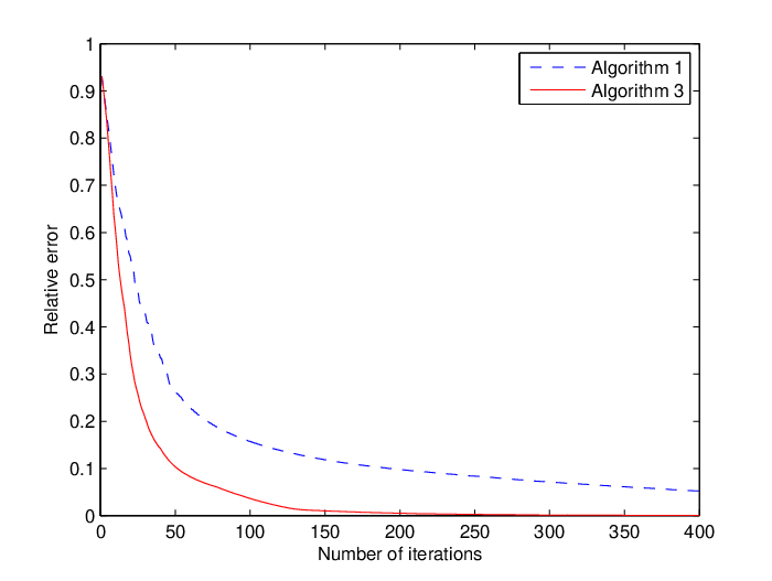
To further illustrate the fast convergence property of Algorithm 3.3, we redo the numerical simulations under the same situation but with exact data. We run iterations for both Algorithm 3.1 and Algorithm 3.3. The relation between the relative errors and the iteration numbers is plotted in Figure 2 which clearly shows that Algorithm 3.3 has the acceleration effect.
Example 4.2.
We next consider the identification of the parameter in the boundary value problem
from an -measurement of the state , where is a bounded domain with Lipschitz boundary, and . This is a benchmark example of nonlinear inverse problems. We assume that the exact solution is in . This problem reduces to solving , if we define the nonlinear operator by , where is the unique solution of (4.2). This operator is well defined on
for some positive constant . It is known that is Fréchet differentiable; the Fréchet derivative of and its adjoint are given by
| (4.4) |
for , where is defined by which is an isomorphism uniformly in ball for small . Moreover, Assumption 3.1 (c) holds for small (see [10]).


We will present our numerical results on with on and
We assume the sough solution is a piecewise constant function as shown in Figure 3 (a) and reconstruct it by using a noisy data with relative noise level . When applying Algorithm 3.1 and Algorithm 3.3 with , we take and
with , where
denotes the total variation of . We use the initial guess and the parameters , , and ; we also take when using Algorithm 3.3. In order to carry out the computation, we need to discretize the problem. We divide into small squares of equal size and solve all partial differential equations involved approximately by a finite difference method. We also discretize so that is replaced by the Fröbenius norm of arrays and is replaced by the discrete total variation given in Section 3.5. The corresponding minimization problems associated with the discrete are solved by the PDHG method which is terminated as long as the relative duality gap is at the -th iteration. In Figure 3 (b) and (c) we report the computational results using Algorithm 3.1 and Algorithm 3.3. The both algorithms give satisfactory reconstruction results. Moreover, Algorithm 3.3 requires significantly less number of iterations than Algorithm 3.1 which demonstrates that Algorithm 3.3 has the acceleration effect.
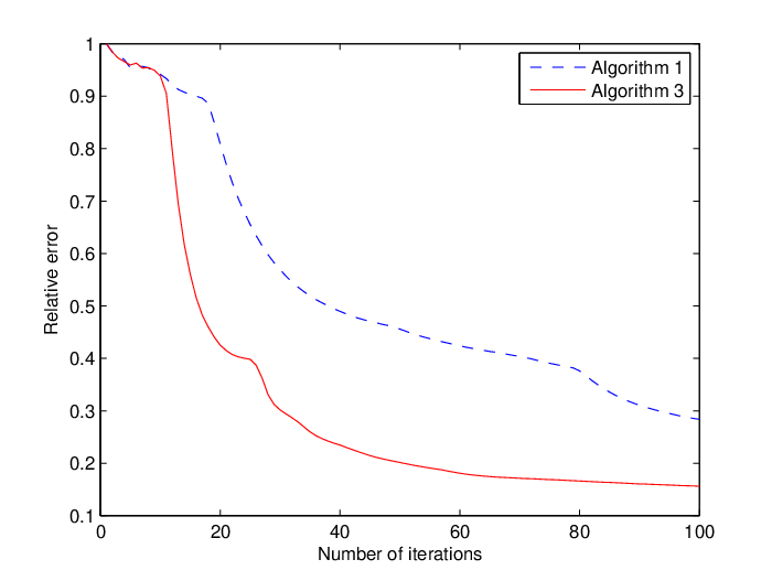
To further illustrate the fast convergence property of Algorithm 3.3, we redo the above computation using exact data. We perform 100 iterations for both Algorithm 3.1 and Algorithm 3.3. The curve of the relative error versus the iteration number is plot in Figure 4 which clearly indicates that Algorithm 3.3 converges faster than Algorithm 3.1.
Acknowledgement
This work is partially supported by the Discovery Project grant of Australian Research Council.
References
- [1] K. J. Arrow, L. Hurwicz, H. Uzawa, Studies in linear and nonlinear programming, Stanford Mathematical Studies in the Social Sciences, vol. II. Stanford University Press, Stanford, 1958
- [2] H. Attouch and J. Peypouquet, The rate of convergence of Nesterov’s accelerated forward-backward method is actually , Preprint 2015.
- [3] A. Beck and M. Teboulle, A fast iterative shrinkage-thresholding algorithm for linear inverse problems, SIAM Journal on Imaging Sciences, 2 (2009), 183–202.
- [4] S. Bonettini and V. Ruggiero, On the convergence of primal–dual hybrid gradient algorithms for total variation image restoration, J Math Imaging Vis., 44 (2012), 236–253.
- [5] R. Bot and T. Hein, Iterative regularization with a geeral penalty term—theory and applications to and TV regularization, Inverse Problems, 28 (2012), 104010.
- [6] H. Brakhage, On ill-posed problems and the method of conjugate gradients, In: Engl HW, Groetsch CW, editors. Inverse and ill-posed problems. Boston (MA): Academic Press 1987, 165–175.
- [7] L. M. Bregman, The relaxation method for finding common points of convex sets and its application to the solution of problems in convex programming, USSR Comput. Math. Math. Phys. 7 (1967), 200–217.
- [8] A. Chambolle and C. Dossai, On the convergence of the iterates of the “fast iterative shrinkage/thresholding algorithm”, J. Optim. Theory Appl., 166 (2015), 968–982.
- [9] A. De Cezaro, M. Haltmeier, A. Leitão, O. Scherzer, On steepest-descent-Kaczmarz methods for regularizing systems of nonlinear ill-posed equations, Appl. Math. Comput., 202 (2008), no. 2, 596–607.
- [10] H. W. Engl, M. Hanke and A. Neubauer, Regularization of Inverse Problems, Mathematics and its Applications, 375. Kluwer Academic Publishers Group, Dordrecht, 1996.
- [11] M. Haltmeier, A. Leitao and O. Scherzer, Kaczmarz methods for regularizing nonlinear ill-posed equations I. Convergence analysis, Inverse Probl. Imaging, 1 (2007), no. 2, 289–298.
- [12] M. Haltmeier, R. Kowar, A. Leitao and O.Scherzer, Kaczmarz methods for regularizing nonlinear ill-posed equations II. Applications, Inverse Probl. Imaging, 1 (2007), no. 3, 507–523.
- [13] M. Hanke, Accelerated Landweber iterations for the solution of ill-posed equations, Numer. Math., 60 (1991), 341–373.
- [14] M. Hanke, A. Neubauer and O. Scherzer, A convergence analysis of the Landweber iteration for nonlinear ill-posed problems, Numer. Math., 72 (1995), 21–37.
- [15] P. C. Hansen and M. Saxild-Hansen, AIR Tools — a MATLAB package of algebraic iterative reconstruction methods, J. Comput. Appl. Math., 236 (2012), 2167–2178.
- [16] M. Hegland, Q. Jin and W. Wang, Accelerated Landweber iteration with convex penalty for linear inverse problems in Banach spaces, Appl. Anal., 94 (2015), 524–547.
- [17] T. Hohage and F. Werner, Iteratively regularized Newton-type methods for general data misfit functionals and applications to Poisson data, Numer. Math., 123 (2013), 745–779.
- [18] K. Ito and B. Jin, Inverse Problems: Tikhonov Theory and Algorithms, World Scientific, Singapore, 2014.
- [19] Q. Jin, Inexact Newton-Landweber iteration in Banach spaces with non-smooth convex penalty terms, SIAM J. Numer. Anal., 53 (2015), no. 5, 2389–2413.
- [20] Q. Jin, Inexact Newton-Landweber iteration for solving nonlinear inverse problems in Banach spaces, Inverse Problems, 28 (2012), 065002 (15pp).
- [21] Q. Jin and U. Tautenhahn, On the discrepancy principle for some Newton type methods for solving nonlinear inverse problems, Numer. Math., 111 (2009), 509–558.
- [22] Q. Jin and W. Wang, Landweber iteration of Kaczmarz type with general non-smooth convex penalty functionals, Inverse Problems, 29 (2013), 085011 (22pp).
- [23] Q. Jin and M. Zhong, On the iteratively regularized Gauss-Newton method in Banach spaces with applications to parameter identification problems, Numer. Math., 124 (2013), 647–683.
- [24] Q. Jin and M. Zhong, Nonstationary iterated Tikhonov regularization in Banach spaces with uniformly convex penalty terms, Numer. Math. 127 (2014), 485–513.
- [25] B. Kaltenbacher and B. Hofmann, Convergence rates for the iteratively regularized Gauss-Newton method in Banach spaces, Inverse Problems, 26 (2010), 035007 (21pp).
- [26] B. Kaltenbacher, A. Neubauer and O. Andreas, Iterative Regularization Methods for Nonlinear Ill-Posed Problems, Radon Series on Computational and Applied Mathematics 6, Walter de Gruyter, Berlin, 2008.
- [27] R. Kowar and O. Scherzer, Convergence analysis of a Landweber-Kaczmarz method for solving nonlinear ill-posed problems, Ill-posed and inverse problems, 253–270, VSP, Zeist, 2002.
- [28] F. Natterer, The Mathematics of Computerized Tomography, SIAM, Philadelphia, 2001.
- [29] Y. Nesterov, A method of solving a convex programming problem with convergence rate , Soviet Mathematics Doklady, 27 (1983), 372–376.
- [30] L. Rudin, S. Osher, and C. Fatemi, Nonlinear total variation based noise removal algorithm, Phys. D, 60 (1992), pp. 259–268.
- [31] F. Schöpfer, A. K. Louis and T. Schuster, Nonlinear iterative methods for linear ill-posed problems in Banach spaces, Inverse problems, 22 (2006), 311-329.
- [32] F. Schöpfer and T. Schuster, Fast regularizing sequential subspace optimization in Banach spaces, Inverse Problems, 25(2009): 015013 (22pp).
- [33] T. Schuster, B. Kaltenbacher, B. Hofmann and K. S. Kazimierski, Regularization Methods in Banach Spaces, Radon Series on Computational and Applied Mathematics 10, Walter de Gruyter, Berlin 2012.
- [34] U. Tautenhahn and Q. Jin, Tikhonov regularization and a posteriori rules for solving nonlinear ill posed problems, Inverse P roblems, 19 (2003), no. 1, 1–21.
- [35] C. Zlinscu, Convex Analysis in General Vector Spaces, World Scientific Publishing Co., Inc., River Edge, New Jersey, 2002.
- [36] M. Zhu and T. F. Chan, An efficient primal–dual hybrid gradient algorithm for Total Variation image restoration, CAM Report 08-34, UCLA (2008)