Semantics and Analysis of DMN Decision Tables
Abstract
The Decision Model and Notation (DMN) is a standard notation to capture decision logic in business applications in general and business processes in particular. A central construct in DMN is that of a decision table. The increasing use of DMN decision tables to capture critical business knowledge raises the need to support analysis tasks on these tables such as correctness and completeness checking. This paper provides a formal semantics for DMN tables, a formal definition of key analysis tasks and scalable algorithms to tackle two such tasks, i.e., detection of overlapping rules and of missing rules. The algorithms are based on a geometric interpretation of decision tables that can be used to support other analysis tasks by tapping into geometric algorithms. The algorithms have been implemented in an open-source DMN editor and tested on large decision tables derived from a credit lending dataset.
Keywords:
Decision Model and Notation, Decision Table, Sweep algorithm1 Introduction
Business process models often encode decision logic of varying complexity, typically via conditional expressions attached either to outgoing flows of decision gateways or to conditional events. The need to separate this decision logic from the control-flow logic [2] and to capture it at a higher level of abstraction has motivated the emergence of the Decision Model and Notation (DMN) [6].
A central construct of DMN is that of a decision table, which stems from the notion of decision table proposed in the context of program decision logic specification in the 1960s [8]. A DMN decision table consists of columns representing the inputs and outputs of a decision, and rows denoting rules. Columns may be typed, meaning that they have an associated domain (or facet). Each rule is a conjunction of basic expressions captured in an expression language known as S-FEEL (Simplified Friendly Enough Expression Language).
The use of DMN decision tables as a specification vehicle for critical business decisions raises the question of ensuring the correctness of these tables, in particular the detection of inconsistent or incomplete DMN decision tables. Indeed, detecting errors in DMN tables at specification time may prevent costly defects down the road during business process implementation and execution.
This paper provides a foundation for analyzing the correctness of DMN tables. The contributions of the paper are: (i) a formal semantics of DMN tables; (ii) a formalization of correctness criteria for DMN tables; and (iii) scalable algorithms for two basic correctness checking tasks over DMN tables, i.e., detection of overlapping rules and detection of missing rules (i.e., incompleteness). The latter algorithms are based on a novel geometric interpretation of DMN tables, wherein each rule in a table is mapped to an iso-oriented hyper-rectangle in an N-dimensional space (where N is the number of columns). Accordingly, the problem of detecting overlapping rules is mapped to that of detecting overlapping hyper-rectangles. Meanwhile, the problem of detecting missing rules is mapped to that of differencing the N-dimensional universe defined by the N columns of a DMN table, and the set of hyper-rectangles induced by its rules. Based on this geometric interpretation and inspired by sweep-based spatial join algorithms [1], the paper presents scalable algorithms for these two analysis tasks. The algorithms have been implemented atop the dmn-js DMN editor and evaluated over decision tables of varying sizes derived from a credit lending dataset.
The rest of the paper is structured as follows. Section 2 introduces DMN and discusses related work. Section 3 presents the formalization of DMN tables and their associated correctness criteria. Section 4 presents the algorithms for correctness analysis while Section 5 discusses their empirical evaluation. Finally, Section 6 summarizes the contributions and outlines future work directions.
2 Background and Related Work
2.1 Overview of DMN Decision Tables
A DMN table consists of columns corresponding to input or output attributes, and rows corresponding to rules. Each column is associated to a type (e.g., a string, a number, or a date), and optionally to a more specific domain of possible values, which we hereby call a facet. Each row has an identifier, one expression for each input column (a.k.a. the input entries), and one specific value for each output column (the output entries). For example, Table 1 shows a DMN table with two input columns, one output column and four rules.
| Income | Size | ||
| A | VG | ||
| B | G | ||
| C | F | ||
Given an input configuration consisting of a vector of values (one entry per column), if every input entry of a row holds true for this input vector, then the vector matches the row and the output entries of the row are evaluated. For example, vector matches rule in Table 1, thus yielding G in the output configuration. To specify how output configurations are computed from input ones, a DMN table may have a hit indicator and a completeness indicator. The hit indicator specifies whether only one or multiple rows of the table may match a given input, and if multiple rules match an input, how should the output configuration be computed. The completeness indicator specifies whether every input configuration must match at least one rule or potentially none. If an input configuration matches two or more rules, this may contradict the hit policy. Similarly, if no rule matches an input configuration, this may contradict the completeness indicator. The former type of contradiction is called overlapping rules while the latter is called missing rule.
2.2 Analysis of DMN Decision Tables
The need to analyze decision tables from the perspective of completeness (i.e., detecting missing rules) as well as consistency and non-redundancy (i.e., detecting overlapping rules) is widely recognized [3]. These two analysis tasks have been tackled using rough sets [7]. However, this approach requires that the domains of the input attributes are boolean or categorical. Numerical attributes need to be previously discretized into intervals. In this paper, we study the problem of analyzing decision tables with arbitrary S-FEEL expressions, meaning that no prior discretization of numerical domains is required.
Prologa [9, 10] is a tool for modeling and executing classical decision tables. It supports the construction of decision tables in a way that prevents overlapping or missing rules. It also supports the optimization of a decision table via rule merging: two rules are merged when all but one of their input entries are identical, and their output entries are also identical. However, Prologa presents the same intrinsic limitation of the rough set approach: it requires columns to have boolean or categorical domains. Hence, numerical domains need again to be discretized into intervals when constructing a decision table.
Signavio’s DMN editor11 1 http://www.signavio.com detects overlapping and missing rules. However, the employed analysis techniques are undisclosed and no empirical evaluation thereof has been reported. Also, the diagnosis of overlapping and missing rules produced by Signavio is unnecessarily large: it often reports the same rule overlap multiple times. This behavior will be further explained in Section 5.
OpenRules22 2 http://openrules.com/ uses constraint satisfaction techniques to analyze business rules, in particular rules encoded in decision tables. While using a general solver to analyze decision tables is an option (e.g., an SMT solver such as Z3 [4]), this approach leads to a boolean output (is the set of rules satisfiable?), and cannot natively highlight specific sets of rules that need to be added to a table (missing rules), nor specific overlaps between pairs of rules that need to be resolved.
3 Formalization
In this section, we provide a logic-based formalization of DMN decision tables, unanmbiguously defining their input/output semantics, and at the same time introducing several analysis tasks focused on correctness checking. As a concrete specification language for input entries in DMN, we consider the S-FEEL language, introduced in the DMN standard itself.
Our formalization is based on classical predicate logic extended with data types, which are needed to capture conditions that employ domain-specific predicates such as comparisons interpreted over the total order of natural numbers. Such formalization is important per sè, as it defines a clear, unambiguous semantics of decision tables, and also as an interlingua supporting the comparison of different analysis techniques.
3.1 Data Types and S-FEEL Conditions
We first introduce the building blocks of decision tables, i.e., the types of the modeled attributes, and conditions over such types expressed using the S-FEEL language. A data type is a tuple , where is an object domain, and is a signature, constituted by a set of predicate symbols, and a set of function symbols (disjoint from ). Each predicate symbol comes with its own arity , and with an -ary predicate that rigidly defines its semantics. Each function symbol comes with its own arity , and with a function that defines its semantics. To make the arity explicit in predicate and function symbols, we use the standard notation and . As usual, we assume that every data type is equipped equality as a predefined, binary predicate interpreted as the identity on the underlying domain. Hence, we will not explicitly mention equality in the signatures of data types. In the following, we show some of the S-FEEL data types33 3 Date/time data types are also supported, but from the logical point of view they can be considered as simple numeric attributes:
- •
– strings.
- •
– boolean attributes.
- •
– integer numbers equipped with the usual comparison predicates and binary operations;
- •
(defined as by replacing the domain with , and by reinterpreting all predicates and functions accordingly) – real numbers equipped with the usual comparison predicates and binary operations.
The set of all such types is denoted by . Since decision tables do not support conditions that combine multiple data types, we can safely assume that the object domains of all types in are pairwise disjoint.
S-FEEL allows one to formulate conditions over types. Such conditions
constitute the basic building blocks for facets and rules, which in
turn are the core of decision tables. The syntax of an
(S-FEEL) condition over type is:
where
is an object and is an -ary function.
Intuitively, S-FEEL supports the following conditions on a given data type :
(i) “” indicates any value, i.e., it holds for every object in . (ii) is a shortcut for “”, and indicates a matching expression, which holds for the object in that corresponds to the result denoted by term . A term, in turn, corresponds either to a specific object in , or to the recursive application of an -ary function in to terms. (iii) is only applicable when is a numeric data type, and indicates a comparison condition, which holds for all objects that are related via the employed comparison predicate to the object resulting from expression . (iv) is only applicable when is numeric, and allows the modeler to capture membership conditions that tests whether an input object belongs to the modeled interval. (v) “” indicates an alternative condition, which holds whenever one of the two conditions and holds.Example 1
The fact that a risk category is either high, medium or low can be expressed by the following condition over : “”. By using to denote the age of persons (in years), the group of people that are underage or old (i.e., having at least years) is captured by condition “”.
3.2 Decision Tables
We are now in the position of defining DMN decision tables. See Table 1 for a reference example. A decision table is a tuple , where:
- •
is the table name.
- •
and are disjoint, finite sets of input and output attributes (represented as strings).44 4 These are called “expressions” in the DMN standard, but we prefer the term “attribute” as it is less ambiguous.
- •
is a typing function that associates each input/output attribute to its corresponding data type.
- •
is a facet function that associates each input/output attribute to a condition over , defining the acceptable objects for that attribute. Facet functions are depicted as “optional lists of values” in Table 1.
- •
is a finite set of rules . Each rule is a pair , where is an input entry function that associates each input attribute to a condition over , and is an output entry function that associates each output attribute an object in .
- •
is a priority function injectively mapping rules in to a corresponding rule number defining its priority. If no priority is explicitly given, in accordance with the standard we assume that the priority is implicitly defined by the graphical ordering in which rule entries appear inside the decision table.
- •
is the completeness indicator, where is the default value and stands for complete table, while stands for incomplete table.
- •
is the (single) hit indicator defining the policy for the rule application, where:
(i) is the default value and stands for unique hit policy, (ii) stands for any hit policy, (iii) stands for priority hit policy, and (iv) stands for first hit policy.
We now informally review the intuitive semantics of rules and of completeness/hit indicators in DMN, moving to the formalization in Section 3.3.
Rule semantics. Intuitively, rules follow the standard “if-then” interpretation. Rules are matched against input configurations, which map the input attributes to objects in such a way that each object
(i) belongs to the type of the corresponding input attribute, and (ii) satisfies the corresponding facet.If, for every input attribute, the assigned object satisfies the condition imposed by the rule on that type, then the rule triggers, and bounds the output attributes to the actual objects mentioned by the rule.
Example 2
Consider the decision table in Table 1. The input configuration where is and is , triggers rule .
Completeness indicator. When the table is declared to be complete, the intention is that every possible input configuration must trigger at least one rule. Incomplete tables, instead, have input configurations with no matching rule.
Hit policies. Hit policies specify how to handle the case where multiple rules are triggered by an input configuration. In particular:
- •
“Unique hit” indicates that at most one rule can be triggered by a given input configuration, thus avoiding the need of handling how to compute the output objects in the case of multiple triggered rules.
- •
“Any hit” indicates that when multiple rules are triggered, they must agree on the output objects, thus guaranteeing that the output is unbambiguous.
- •
“Priority hit” indicates that whenever multiple rules trigger, then the output is unambiguously computed by only considering the contribution of the triggered rule that has highest priority.
- •
“First hit” can be understood as a variant of the priority hit, in which priority is implicitly obtained from the ordering in which rules appear in the decision table. Hence, this case is subsumed by that of priority hit.
- •
“Collect” implies that multiple rules can match an input configuration and when this is the case, all matching rules are fired the the resulting output configurations are aggregated. Aggregation is orthogonal to correctness checking, and thus we leave the “Collect” policy outside the scope of the formalization below.
3.3 Formalization of Rule Semantics and of Analysis Tasks
We first define how conditions map to corresponding
formulae. Since each condition is applied to a single input
attribute, the corresponding formula has a single free variable
corresponding to that attribute.
Given a condition over
type , the condition formula for
, written , is a formula using
predicates/functions in and objects from ,
and possibly mentioning a single free variable, constructed as follows:
As usual, we also use notation to explicitly mention
the free variable of the condition formula.
Example 3
Consider the S-FEEL conditions in Example 1. The condition over the risk category is . The condition formula person ages is instead: .
With this notion at hand, we now formalize the notions of correctness of rule specifications, semantics of rules, and semantics of completeness and hit indicators. These notions are building blocks for an overall notion of table correctness.
Let be a decision table with input attributes , output attributes , and rules . We use variables for objects matching the input attributes, and variables for those matching the output attributes.
Facet correctness. We first consider the Facet correctness of , which intuitively amounts to check whether all the mentioned input conditions and output objects are compatible with their corresponding attribute facets.
Given an attribute and a corresponding input variable , the fact that is legal for is defined as:
We use this notion in combination with a condition over , so as to check whether an input variable matches with :
Note that for output objects, above is a test where is equated to the output object.
This derived predicate, in turn, can be used to identify whether is compatible with , i.e., whether the condition is specified in such a way that can potentially trigger, or is instead contradictory with the facet attached to :
Rule semantics. A rule is triggered by a configuration of input objects whenever each such object matches with the corresponding input condition:
Two configurations and of input and output objects are input-output related by a rule if the rule is triggered by the input configuration, and binds the output as specified by the output configuration:
Completeness. When declaring that a table is (in)complete, there is no guarantee that the specified rules guarantee this property. To check whether this is indeed the case, we introduce a formula that holds whenever each possible input configuration triggers at least one rule:
Hit policies. We start with the unique hit policy, which requires that each input configuration triggers at most one rule. This can be formalized as follows:
We then continue with the any hit policy. Here multiple rules may be triggered by the same input configuration, but if so, then they must agree on the output. This can be formalized as follows:
We now consider the case of priority hit policy. This requires to reformulate the rule semantics, so as to consider the whole decision table and the priority of the rules. In particular, with this hit policy a rule is triggered with priority by an input configuration if it is triggered by in the sense specified above, and no rule of higher priority is triggered by the same input :
With this policy, the relationship between input and output configurations can be lifted from the single-rule case discussed above to the whole decision table by isolating the highest-priority rule that matches with the input configuration, and by considering its output:
Finally, we observe that the priority hit policy may create a situation in which some rules are never triggered. This happens when other rules of higher priority have more general input conditions. We formalize this notion by introducing a formula dedicated to check when a rule is masked by another rule :
Correctness formula. We now combine the previously defined formulae into a single formula that captures the overall correctness of a decision table.
We say that is correct if the following conditions hold:
- 1.
Every table cell, i.e., every input condition or output object, is legal for the corresponding attribute (considering the attribute type and facet).
- 2.
The completeness indicator corresponds to iff the table is indeed complete.
- 3.
The rules are compatible with the hit policy indicator:
- (a)
if the hit policy is , each input configuration triggers at most one rule;
- (b)
if the hit policy is , all overlapping rules (i.e., rules that could simultaneously trigger) have the same output;
- (c)
if the hit policy is , all rules are “useful”, i.e., no rule is masked by a rule with higher priority.
- (a)
Based on the previously introduced formulae, we formalize correctness as:
| (1) | ||||
| (2) | ||||
| (3a) | ||||
| (3b) | ||||
| (3c) |
Global input-output formula. We combine the previously defined formulae into a single formula that captures the overall input-output relation induced by . This is done by exploiting the notion of input-output related configurations by a rule, so as to cover the entire table. Specifically we say that an input configuration and an output configuration are input-output related by if:
- 1.
the hit policy is either or , and there exists a rule that relates to (in the case of any hit policy, there could be many, but they establish the same input-output relation, so it is sufficient to pick one of them);
- 2.
the hit policy is , and there exists a rule relating to without any other rule of higher priority that is triggered by (is such a rule exists, then it is such rule that has to be selected to relate input-output).
This is formalized as follows:
| (1) | ||||
| (2) |
4 Algorithms
We now introduce algorithms to handle the two main analysis tasks introduced in the previous section: detecting overlapping rules and (in)completeness. The proposed algorithms rely on a geometric interpretation of a DMN table. Every rule in a table is seen as an iso-oriented hyper-rectangle in an N-dimensional space (where N is a number of columns). Indeed, an input entry in a rule can be seen a constraint over one of the columns (i.e. dimensions). In the case of a numerical column, an input entry is an interval (potentially with an infinite upper or lower bound) and thus it defines a segment or line over the dimension corresponding to that column. In the case of a categorical column, we can map each value of the column’s domain to a disjoint interval – e.g. “Refinancing” to [0..1), “Card payoff” to [1..2), “Car leasing” to [2..3), etc. – and we can see an input entry under this column as defining a segment (or set of segments) over the dimension corresponding to the column in question. The conjunction of the entries of a row hence defines a hyper-rectangle, or potentially multiple hyper-rectangles in the case of a multi-valued categorical input entry (e.g. {“Refinancing”, “Car leasing”}). The hyper-rectangles are iso-oriented because only constraints of the form “attribute operator literal” are allowed in S-FEEL and such constraints define iso-oriented lines or segments.
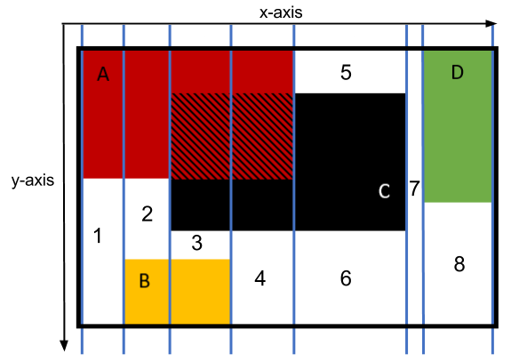
For example, the geometric interpretation of Table 1 is shown in Figure 1. The two dimensions, and , represent the two input columns (Annual income and Loan size) respectively. The table contains 4 rules: , , , and . Some of them are overlapping. For example, rule overlaps with rule . Their intersection is the rectangle . The table also contains missing values. For example, vector does not match any rule in Table 1.
The algorithms are presented for numeric columns. Minor adaptations (not discussed here) allow these algorithms to handle categorical columns as well.
4.1 Finding Overlapping Rules
Algorithm 1 finds overlapping rules in a DMN table. This algorithm is an extension of line-sweep algorithm for two-dimensional spatial joins proposed in [1]. The idea of this latter algorithm is to pick one dimension (e.g. x-axis), project all objects into this dimension, and then sweep an imaginary line orthogonal to this axis (i.e. parallel to the y-axis). The line stops at every point in the x-axis where either an object starts or ends. When the line makes a “stop”, we gather all objects that intersect the line (the active list). These objects overlap along their x-axis projection. In [1], it is then checked if the objects also overlap in the y-axis, and if so they are added to the result set (i.e. the objects overlap). Algorithm 1 extends this idea to N dimensions. The algorithm takes as input:
- 1.
ruleList, containing all rules of the input DMN table;
- 2.
i, containing the index of the column under scrutiny;
- 3.
N, representing the total number of columns;
- 4.
OverlappingRuleList, storing the rules that overlap.
The algorithm starts analyzing the first column of the table (axis ). All rules are projected over this column. Note that the projection of a rule on a column is an interval. We indicate the projection of rule over axes and with and respectively. All the intervals are represented in terms of upper and lower bounds. The bounds are sorted in ascending order (line 7). The algorithm iterates over the list of sorted bounds (line 8). In the case of Figure 1, the rules projected over the axis correspond are:
Considering the rules above, the algorithm first analyzes the lower bound of . Therefore, is added to an active list of intervals for the first column , , since the bound processed is a lower bound (line 13). Next, the algorithm processes the lower bound of and is added to . Then, the lower bound of is processed and is added to . Finally, the algorithm processes the upper bound of . Every time an upper bound of an interval is processed (line 9), the following column of the table is analyzed (in this case ) by invoking findOverlappingRules recursively (line 10).
All the intervals projections on of the rules corresponding to intervals contained in (in our example , , and ) are represented in terms of upper bounds and lower bounds:
The bounds are sorted in ascending order. The algorithm iterates over the list of sorted bounds. Considering the intervals above, the algorithm first encounters the lower bound of . Therefore, is added to the active list of intervals for the second column , . Next, the algorithm processes the lower bound of and adds to . Then, the upper bound of is processed. Since there is no other column in the table, this means that all the rules corresponding to the intervals in overlap. At the end of each recursion, the interval corresponding to the current bound is removed from the current active list (line 11). In addition, when the last column of the table is processed (line 1), the algorithm checks whether the identified set of overlapping rules is contained in one of the other sets produced in a previous recursion (lines 3). If this is not the case, the new set of overlapping rules is added to the output list overlappingRuleList (line 4). In this way, the procedure outputs maximal sets of overlapping rules having a non-empty intersection stored in overlappingRuleList (line 16).
4.2 Finding Missing Rules
Algorithm 2 describes the procedure for finding missing rules, which is also based on the line-sweep principle. The algorithm takes as inputs 5 parameters:
- 1.
ruleList, containing all rules of the input DMN table;
- 2.
missingIntervals, storing the current missing intervals;
- 3.
i, containing the index of the column under scrutiny;
- 4.
N, representing the total number of columns;
- 5.
MissingRuleList, storing the missing rules.
The algorithm starts analyzing the first column of the table (axis ). Consider again the projection of the table in Figure 1 on :
Upper and lower bounds of each interval are sorted in ascending order (line 3). The algorithm iterates over the list of sorted bounds (line 4).
Considering the rules above, the algorithm first analyzes the lower bound of . Therefore, is added to an active list of intervals for the first column , . An interval is added to the active list only if its lower bound is processed (line 15). If the upper bound of an interval is processed, the interval is removed from the list (line 17). Next, the algorithm processes the lower bound of . Since is not empty, is not added to yet (line 11). Starting from the interval (line 12) having the lower bound of as lower bound and the lower bound of as upper bound, the following column of the table is analyzed (in this case ) by invoking findMissingRules recursively (line 13). All the interval projections on of the rules corresponding to intervals contained in (in our example only ) are represented in terms of upper and lower bounds, obtaining in this case the following simple situation:
The bounds are sorted in ascending order. The algorithm iterates over the list of sorted bounds. The first bound taken into consideration is the lower bound of so that is added to (since is empty). Since this bound corresponds to the minimum possible value for , there are no missing values between the minimum possible value for and the lower bound of (line 5). Next, the algorithm processes the second bound in that is the upper bound of . Considering that the upper bound of is the last one in , the algorithm checks if this value corresponds to the maximum possible value for (line 5). Since this is not the case, this means that there are missing values in the area between the upper bound of and the next bound over the same column (in this case area 1). The algorithm checks if the identified area is contiguous to an area of missing values previously found (line 7). If this is the case the two areas are merged (line 8). If this is not the case, the area is added to a list of missing value areas (line 10). In our case, area 1 is added to a list of missing value areas. Note that the algorithm merges two areas of missing values only when the intervals corresponding to one column are contiguous and the ones corresponding to all the other columns are exactly the same. In the example in Figure 1, areas 4 and 6 are merged.
At this point, the recursion ends and the algorithm proceeds analyzing the intervals in the projection along the axis. The last bound processed was the lower bound of , so that is added to . Next, the algorithm processes the lower bound of (since is not empty, is not added to yet). Starting from the interval having the lower bound of as lower bound and the lower bound of as upper bound, the following column of the table is analyzed (in this case ) again through recursion.
All intervals projections on of the rules corresponding to intervals contained in (in this case and ) are represented in terms of upper and lower bounds:
The bounds are sorted in ascending order. The algorithm iterates over the list of sorted bounds. Considering the rules above, the algorithm first processes the lower bound of so that is added to ( is empty). Then, the upper bound of is processed. When the algorithm reaches the upper bound of an interval in a certain column the interval is removed from the corresponding active list. Therefore, is removed from . Next, the lower bound of is processed. Since is empty, the algorithm checks if the previous processed bound is contiguous with the current one (line 5). Since this is not the case, this means that there are missing values in the area between the upper bound of and the next bound over the same column (in this case area 2). The algorithm checks if the identified area is contiguous to an area of missing values previously found. If this is the case, the two areas are merged. If this is not the case, the area is added to a list of missing value areas (in our case area 2 is added to a list of missing value areas). The list of missing areas stored in missingRuleList is returned by the algorithm (line 19).
5 Evaluation
We implemented the algorithms on top of dmn-js: the open-source rendering and editing toolkit of Camunda DMN.55 5 https://camunda.org/ In it current version, dmn-js does not support correctness verification. Our dmn-js extension with verification features can be found at https://github.com/ulaurson/dmn-js and a deployed version is available for testing at http://kodu.ut.ee/~ulaurson/DMN/.
For the evaluation, we created decision tables from a loan dataset of LendingClub -- a peer-to-peer lending marketplace.66 6 Dataset available at https://www.lendingclub.com/info/download-data.action The employed dataset contains data about all loans issued in 2013-2014 (23 5629 loans). For each loan, there are attributes of the loan itself (e.g., amount, purpose), of the lender (e.g., income, family status, property ownership), and a credit grade (A, B, C, D, E, F, G).
Using Weka [5], we trained decision trees to classify the grade of each loan from a subset of the loan attributes. We then translated each trained decision tree into a DMN table by mapping each path from the root to a leaf of the tree into a rule. Using different attributes and pruning parameters in the decision tree discovery, we generated DMN tables containing approx. 500, 1000 and 1500 rules and 3, 5 and 7 columns (nine tables in total). The 3-dimensional (i.e. 3-column) tables have one categorical and two numerical input columns; the 5-dimensional tables have two categorical and three numerical input columns, and the 7-dimensional tables has two categorical and five numerical input columns.
By construction, the generated tables do not contain overlapping or missing rules. To introduce missing rules in a table, we selected of the rules. For each of them, we then randomly selected one column, and we injected noise into the input entry in the cell in the selected column by decreasing its lower bound and increasing its upper bound in the case of a numerical domain (e.g. interval [3..6] becomes [2..7]) and by adding one value in the case of a categorical domain (e.g. { Refinancing, CreditCardPayoff } becomes { Refinancing, CreditCardPayoff, Leasing }). These modifications make it that the rule will overlap others. Conversely, to introduce missing rule errors, we selected of the rules, picked a random column for each row and “shrank” the corresponding input entry.
We checked each generated table both for missing and incomplete rules and measured execution times averaged over 5 runs on a single core of a 64-bit 2.2 Ghz Intel Core i5-5200U processor with 16GB of RAM. The results are shown in Table 2. Execution times for missing rules detection are under 2 seconds, except for the 7-columns tables with 1000-1500 rules. The detection of overlapping rules leads to higher execution times, due to the need to detect sets of overlapping rules and ensure maximality. The execution times for overlapping rules detection on the 3-columns tables is higher than on the 5-columns tables because the 5-columns tables have less rule overlaps. This is because there are proportionally less categorical columns in the 5-columns tables than in the 3-columns ones, and the modifications made to categorical columns create more overlaps.
In addition to implementing our algorithms, we implemented algorithms designed to produce the same output as Signavio. In Signavio, if multiple rules have a joint intersection (e.g. rules {r1, r2, r3}) the output contains an overlap entry for the triplet {r1, r2, r3} but also for the pairs {r1, r2}, {r2, r3} and {r1, r3} (i.e. subsets of the overlapping set). Furthermore, the overlap of pair {r1, r2} may be reported multiple times if r3 breaks into multiple hyper-rectangles (and same for {r2, r3} and {r1, r3}). Meanwhile, our approach produces only maximal sets of overlapping rules with a non-empty intersection.
Table 3 shows the number of sets of overlapping rules and the number of missing rules identified by our approach vs. Signavio’s one. In all runs, both the number of overlapping and missing rules is drastically lower in our approach.
| 3 columns | 5 columns | 7 columns | |||||||
|---|---|---|---|---|---|---|---|---|---|
| #rules | 499 | 998 | 1 492 | 505 | 1 000 | 1 506 | 502 | 1 019 | 1 496 |
| overlapping time | 297ms | 6 475ms | 24 530ms | 200ms | 1 621ms | 5 374ms | 5 715ms | 6 793ms | 30 736ms |
| missing time | 160ms | 611ms | 1 672ms | 163ms | 820ms | 1 942ms | 2 173ms | 7 029ms | 18 263ms |
| 3 columns | 5 columns | 7 columns | ||||||||
|---|---|---|---|---|---|---|---|---|---|---|
| #rules | 499 | 998 | 1 492 | 505 | 1 000 | 1 506 | 502 | 1 019 | 1 496 | |
| #overlapping | our approach | 131 | 447 | 812 | 110 | 225 | 378 | 139 | 227 | 371 |
| rule sets | Signavio | 1 226 | 10 920 | 23 115 | 679 | 3 692 | 8 921 | 23 175 | 22 002 | 62 217 |
| #missing | our approach | 117 | 330 | 726 | 136 | 254 | 462 | 134 | 322 | 518 |
| rules | Signavio | 668 | 2 655 | 5 386 | 563 | 2 022 | 4 832 | 5 201 | 18 076 | 43 552 |
6 Conclusion and Future Work
This paper presented a formal semantics of DMN decision tables, a notion of DMN table correctness, and algorithms that operationalize two core elements of this correctness notion: the detection of overlapping rules and of missing rules. The algorithms have been implemented atop the DMN toolkit dmn-js. An empirical evaluation on large decision tables has shown the potential for scalability of the proposed algorithms and their ability to generate non-redundant feedback that is more concise than the one generated by the Signavio DMN editor.
The proposed algorithms rely on a geometric interpretation of rules in decision tables, which we foresee could be used to tackle other analysis problems. In particular, we foresee that the problem of simplification of decision tables (rule merging) could be approached from a geometric standpoint. Indeed, if we see the rules as hyperrectangles, the problem of table simplification can be mapped to one of finding an optimal way of merging hyperrectangles with respect to some optimality notion. Another direction for future work is to extend the proposed formal semantics to encompass other aspects of the DMN standard, such as the concept of Decision Requirements Graphs (DRGs), which allow multiple decision tables to be linked in various ways.
Acknowledgement. This research was partly funded by an Institutional Grant of the Estonian Research Council.
References
- [1] Lars Arge, Octavian Procopiuc, Sridhar Ramaswamy, Torsten Suel, and Jeffrey Scott Vitter. Scalable sweeping-based spatial join. In VLDB, 1998.
- [2] Kimon Batoulis, Andreas Meyer, Ekaterina Bazhenova, Gero Decker, and Mathias Weske. Extracting decision logic from process models. In CAiSE’15.
- [3] CODASYL Decision Table Task Group. A Modern appraisal of decision tables : a CODASYL report. ACM, 1982.
- [4] Leonardo Mendonça de Moura and Nikolaj Bjørner. Z3: an efficient SMT solver. In Proc. of TACAS, pages 337–340. Springer, 2008.
- [5] Mark A. Hall, Eibe Frank, Geoffrey Holmes, Bernhard Pfahringer, Peter Reutemann, and Ian H. Witten. The WEKA data mining software: an update. SIGKDD Explorations, 11(1):10–18, 2009.
- [6] Object Management Group. Decision Model and Notation (DMN) 1.0, 2015.
- [7] Zdzislaw Pawlak. Decision tables – a rough set approach. Bulletin of the EATCS, 33:85–95, 1987.
- [8] Udo W. Pooch. Translation of decision tables. Comp. Surv., 6(2):125–151, 1974.
- [9] Jan Vanthienen and Elke Dries. Illustration of a decision table tool for specifying and implementing knowledge based systems. International Journal on Artificial Intelligence Tools, 3(2):267–288, 1994.
- [10] Jan Vanthienen, Christophe Mues, and Ann Aerts. An illustration of verification and validation in the modelling phase of KBS development. Data Knowl. Eng., 27(3):337–352, 1998.