Regular black holes: Guilfoyle’s electrically charged solutions with a perfect fluid phantom core
Abstract
Regular black hole solutions are found among the Guilfoyle exact solutions. These are spherically symmetric solutions of general relativity coupled to Maxwell’s electromagnetism and charged matter where the metric potentials and electromagnetic fields are related in some particularly simple form. We show that, for certain ranges of the parameters, there are objects which correspond to regular charged black holes, whose interior region is filled by an electrically charged phantomlike fluid, or, in the limiting case, a de Sitter false vacuum fluid, and whose exterior region is Reissner-Nordström. The boundary between both regions is a smooth boundary surface, except in the limiting case where the boundary is made of a massless electrically charged spherically symmetric coat. The main physical and geometrical properties of such charged regular solutions are analyzed.
Keywords:
Regular black holes; null and timelike boundaries; Einstein-Maxwell equationspacs
04.70.Bw, 04.20.Jb, 04.40.Nr, 04.40.DgI Introduction
Solutions of Einstein-Maxwell with matter equations are of importance as they not only represent a class of solutions in general relativity but also give hints to the behavior of solutions with other type of fields. Electric charged compact objects, starlike, solutions have been constructed by Guilfoyle in [1]. The interpretation of the fluid content in these solutions has appeared in [2], and part of the spectrum of the solutions received a global interpretation in [3, 4].
On the other hand, a class of compact objects that has been of interest are regular black holes, i.e., black holes that, contrary to the usual Schwarzschild and Reissner-Nordström black holes, do not possess curvature singularities at the center. In these regular black holes a well-behaved interior replaces the singularity.
The first work on regular black holes is due to Bardeen [5] whose regular black hole was put on a firm footing in [6]. Dymnikova [7] constructed a regular black hole solution whose interior matter is an anisotropic fluid obeying a de Sitter equation of state, , where and are the energy density and pressure of the fluid, respectively, that asymptotically approached the Schwarzschild spacetime. Other regular black hole solutions have been found in [8, 9] where the interior region is a de Sitter core that can be matched to a Reissner-Nordström exterior metric thanks to an energyless charged layer at the boundary surface (see also [10]). Regular black holes with nonlinear electrodynamics sources appear in, e.g., [11, 12, 13]. Stability of these black holes appeared in [14, 15]. Regular black holes in different theories of gravity also appeared in [16, 17], and in nonminimal theories in [18].
An important class of regular black holes is the class of phantom matter black holes. Phantom matter is characterized by a perfect fluid for which . Fluids satisfying such a condition may represent the dark energy sector of the Universe. The property of phantom matter to act as a negative effective mass turns it into a natural candidate to build models of compact objects and, in particular, to build black hole solutions free from singularities. This motivated several works reporting on black holes with phantom matter, some of them regular, see [19, 20, 21, 22, 23, 24, 25, 26, 27, 28].
Now, electric charged matter provides repulsion, but in general this electric repulsion is not enough to furnish regularity at the center. However, electrically charged matter made of a phantom perfect fluid might indeed be suitable to produce enough antigravity in order to form a regular core. Thus it is worth exploring the possibility that the Guilfoyle solutions [1] contain a subset of regular electrical black holes with a phantom perfect fluid core.
In the present work we analyze in detail the Guifoyle model for electrically charged matter [1] and show that within a certain range of the parameters of the model there are indeed regular black holes whose central core is made by a charged perfect fluid obeying an equation of state representing phantom matter for which .
The layout of the paper is as follows. In Sec. II we present the basic equations describing a spherically symmetric electrically charged perfect fluid matter distribution satisfying some simplifying assumptions, that define the systems. We give explicitly the interior and exterior solutions with the appropriate boundary conditions and display the class of the Guilfoyle solutions that is of interest here. We also show the conditions on the solutions necessary to make them black holes. Section III is dedicated to analyzing the phantom regular charged black hole solutions we have found, presenting their main properties, and comparing the present solutions to other regular black hole solutions found in the literature. In Sec. IV a particular limit of the regular black holes analyzed, where the core is made of de Sitter material and there is a massless charged layer at the Cauchy horizon, is studied. Then in Sec. V the spectrum of the free parameters of the solutions that yields regular black holes is analyzed in detail. In the first part, we study the behavior of the mass and other free parameters in terms of the radius and energy density of the solutions. The second part contains the display of the regions of the parameter space where regular black holes can be found. We also comment on some interesting cases including the ones analyzed in the previous sections. Finally, in Sec. VI we conclude.
II Guilfoyle solutions and black hole conditions
II.1 Spherical static Weyl-Guilfoyle systems and equations
The matter source is a static charged fluid distribution with spherical symmetry. The metric is conveniently written in the form
| (1) |
where are spherical symmetric coordinates, and the functions and depend on the radial coordinate only. The fluid is characterized by its energy density , isotropic pressure , electric charge density , and four-velocity . The electromagnetic gauge field assumes the form
| (2) |
where is the electric potential.
Two important auxiliary quantities are the mass inside a sphere of radius
| (3) |
and the electric charge inside a sphere of radius ,
| (4) |
The system we study here is a case of the Weyl-Guilfoyle-type systems for which the metric potential and the electric potential are functionally related through a particular Weyl-Guilfoyle relation [1] (see also [2]), namely, , with and being arbitrary constants and . Now, the parameter can be absorbed into the electric potential , and so without loss of generality one can set . Thus,
| (5) |
with being an arbitrary constant called the Guilfoyle parameter.
Using the Einstein-Maxwell equations one finds the set of equations for this system (we use units in which the gravitational constant and the speed of light are set to one). The Einstein part of the equations furnishes the following relations,
| (6) | |||
| (7) |
where a prime denotes the derivative with respect to the radial coordinate . With the definition of the total charge inside a sphere of radius , see Eq. (4), the only nonzero component of the Maxwell equation yields , where an integration constant was set to zero. From Eq. (5) we can write in terms of as . With this, the amount of electric charge inside a spherical surface of radius , Eq. (4), is then given by
| (8) |
The electric charge is then obtained once we have the metric functions and .
II.2 Guilfoyle solutions
II.2.1 Interior solution
The interior goes up to a certain radius , say. Guilfoyle’s solutions are found under the assumption that the effective energy density is a constant,
| (10) |
where , a characteristic length associated to the inverse of the total energy density, is a constant to be related to the parameters of the exterior solution, and , by the junction conditions of the metric at the surface . With this hypothesis, Guilfoyle [1] found an exact solution given by
| (11) |
| (12) |
| (13) |
| (14) |
| (15) | |||||
| (16) |
The auxiliary functions are
| (17) |
| (18) |
The function is defined by
| (19) |
and the integration constants and are given by
| (20) |
| (21) |
where
| (22) |
| (23) |
The constants and are found through the junction conditions. As one can check, the above solution is valid for all , the limiting case yielding the uncharged () Schwarzschild interior solution. We are not interested in negative .
II.2.2 Exterior solution
The solution of Einstein-Maxwell field equations, Eqs. (6)-(8), for the external region, , is given by
| (24) |
| (25) |
| (26) |
| (27) |
| (28) |
| (29) |
and the auxiliary functions are
| (30) |
| (31) |
which is the Reissner-Nordström solution. Note that, by continuity on the surface , the metric functions yield . Also one must have , , and , and being the total mass and total charge of the exterior spacetime.
II.2.3 Junction conditions
To do the matching properly, we start by imposing the junction condition that the metric should be continuous at the boundary surface . In fact, by joining the interior metric function in Eq. (11) with the coefficient of the exterior metric given by (25), it is found [1] that
| (32) |
Another junction condition arises by using the continuity of the metric coefficient, the continuity of its first derivative at , and Eq. (8). Then one gets
| (33) |
where the fact that was also taken into account, and positive is assumed without loss of generality.
II.2.4 Some constraints
Equations (32)-(33) are two constraints to the five free parameters of the solutions, , , , , and . We now investigate some constraints on these parameters.
Using Eqs. (32)-(33) it is possible to treat the Guilfoyle parameter and the mass of the solution as a function of the other parameters of the theory, namely, and . Relation (33) implies may be zero or negative in some range of the parameters. However, to avoid imaginary electromagnetic fields, we are interested just in solutions for which
| (34) |
and so we use Eq. (33) to constrain the range of the parameters and . The condition requires that
| (35) |
II.3 Black hole conditions
We are looking for regular black holes. The conditions for the solutions to be regular are subtle and can be found numerically. The conditions for the solutions to be black holes are simple and can be stated now. The first condition to check is the presence of horizons. Namely, the expressions for the Cauchy and event horizon radii of the Reissner-Nordström solution exterior to the matter,
| (36) |
| (37) |
respectively, have to produce real numbers. Then the overcharged solutions are discarded and we have the constraint,
| (38) |
Thus the existence of and for the electrically charged solutions guarantees that the solutions are black holes.
Moreover, the radius of the boundary surface cannot be larger than, or at most, the gravitational radius , i.e., . However, inequality (38) together with condition (35) imply that the value of cannot be in the region between and . Additionally, the boundary conditions impose that cannot be equal to , with one special case as an exception, when and at the extremal regime , which means . The constraint for is then
| (39) |
the equality holding in the limit of . This result and Eq. (37) give
| (40) |
the equality holding in the limit of .
III Regular nonextremal black holes with charged phantom matter
In testing for regularity of the solutions, we find that there is a region of the parameter space which corresponds to regular black holes for small characteristic length , namely,
| (41) |
From now on we write the parameters of the problem as parameters without units, mainly we use the total charge as the quantity to which the other parameters are gauged. Since from Eq. (10), , small characteristic length means sufficiently large total energy density, i.e., the configurations are compact relative to the electric charge. Or, if one prefers, the configurations are heavily charged in comparison.


Besides , another useful parameter for our analysis is the ratio , which is the ratio of the radius of the matter distribution to the energy density parameter . For very compacted charged spheres, typically, for , the fluid energy density assumes negative values at some . On the other hand, for
| (42) |
from below, the energy density is positive, while the pressure is negative everywhere inside the central core. For solutions in this range one has , i.e.,
| (43) |
which means that the fluid is composed of a phantom matter with electric charge. This is a Guilfoyle phantom fluid.
To show that these configurations are indeed black holes, regular ones, we focus on the physical quantities , , , , and and plot them as functions of . The potential is not necessary to plot as it is given by Eq. (13). We also plot and which are useful quantities. As a typical class of configurations we consider the case
| (44) |
According to Eq. (35), the maximum value for is , so in this case the upper limit is then
| (45) |


In Figs. 2-7 we display the behavior as a function of of the above-mentioned physical quantities for four different values of , namely, , this latter number being the maximum value possible, see Eq. (45).
In Figs. 2-2 the plots of the metric potentials and are shown. Clearly there are no curvature singularities, i.e., the black holes are regular. The curve for (dotted line) corresponds to a regular black hole with a de Sitter core, to be treated separately. The small difference among the curves of Figs. 2 and 2 is related to the fact that we considered regular black holes of almost the same sizes, i.e., with values of very close to each other. Although the values of the mass are relatively close to , these regular black holes are far from being extremal as and differ substantially. These facts can be found in Table I, which shows the values of the mass , the Cauchy and event horizon radii, and , respectively, for some chosen values of , with fixed. It is clear from the table that , i.e., the matter radius is inside the Cauchy horizon.
| 0.720000 | 1.02622 | 0.795724 | 1.25672 |
| 0.730000 | 1.03072 | 0.780939 | 1.28051 |
| 0.740000 | 1.03587 | 0.765622 | 1.30613 |
| 0.750000 | 1.04167 | 0.750000 | 1.33333 |

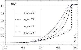


In Fig. 4 the energy density is displayed for the mentioned range of parameters. We see that within this range it is positive. The curve with (dotted line) is flat, has a sharp drop at the boundary, and corresponds to a de Sitter core. Due to its particular interest it is studied separately. For smaller values of the solutions are less interesting, as they have negative energy densities. In Fig. 4 the pressure is shown. The values are negative and higher in modulus than the energy density . The fluid is a phantom fluid. The curve with (dotted line), that is flat and drops sharply to zero at the boundary corresponds to a de Sitter core. In Figs. 5 the charge density profiles for the given range of parameters are shown. Finally, the behavior of the auxiliary functions and is shown in Figs. 6 and 7, respectively.
The conformal Carter-Penrose diagram of this regular black hole is shown in Fig. 8. The external region () is Reissner-Nordström, possessing a Cauchy and an event horizon, and , respectively. In the external region there are three distinct regions indicated in the figure by I, II, and III. The internal regular region, indicated by R in the diagram, is filled by a distribution of charged matter for which the pressure is negative and larger in absolute value than the energy density in the central core.
IV Regular black holes with a de Sitter core and a massless charged layer at the Cauchy horizon
Within this set of Guilfoyle solutions there are also regular black holes with a de Sitter core whose matching to the exterior region occurs at the Cauchy horizon, , which is a null, i.e., lightlike, surface. The interior fluid, , is uncharged, satisfying a de Sitter equation of state , so that
| (46) |
for this fluid. It is a false vacuum de Sitter core, the limiting case of a phantom fluid . The boundary of this de Sitter core, , is a layer of zero mass but nonzero charge. Thus, all the electric charge is on such a surface.
Let us show from the equations that this regular black hole solution exists.
By inspection, or otherwise, it is seen that this solution exists when . Since by Eq. (36), , using Eq. (32), we obtain . This equation gives two solutions. One is , which is satisfied for all and is in fact a singular black hole. The other solution is
| (47) |
and is satisfied only for . This latter is the solution that yields regular black holes. Thus
| (48) |
for this black hole.
Let us now discuss the features of the three different regions of this regular black hole.
(i) The region : In this region the interior fluid is uncharged, satisfying a de Sitter equation of state.
Indeed, in the limit the ratio tends to unity, . One can find this result by taking the limit in Eqs. (12)-(21) with the help of Eqs. (32)-(33).
To be specific, we see from Eq. (33) that for and for , see Eq. (48), the parameter diverges with . Hence, Eq. (20) implies that the following limit, , is finite. Similarly, it follows from Eq. (21) that the constant goes to zero with . Therefore, for , the function defined in Eq. (19) is finite and nonzero. Then, in the limit the solution for is
| (49) | |||
| (50) | |||
| (51) |
Thus these black holes have a central de Sitter vacuum up to , .
Note that generically, the metric function can be made equal to by a redefinition of the time coordinate. Note also that for , a case that follows outside the configurations we are studying (see Eq. (48)), for all and we are in the presence of a quasiblack hole.

(ii) The region : In this region one has an electrically charged massless layer. Indeed, in the limit , and the function defined in Eq. (19) goes to zero as . Then the charge density diverges at , but the total charge is finite,
| (52) |
(iii) The region : By construction this region is the Reissner-Nordström vacuum.
Thus, we have shown that a regular black hole solution with a de Sitter core and a massless electrically charged layer at the Cauchy horizon is a solution of the equations.
The resulting metric and fluid functions for this extremal case correspond to the dotted curves of Figs. 2-7. Those plots show the particular case . Worth noting is the graph for (dotted curve of Fig. 5), which is essentially for , and diverges at . Its integration gives , see Fig. 7, i.e., it is zero for and for , indicating that has similar properties to the Dirac delta function. This special case is identical to a special case of the regular charged black holes found in [8], see also [10]. The conformal Carter-Penrose diagram for these regular black holes is shown in Fig. 9. In the external region there are two distinct regions indicated in the figure by I and II. The internal regular region, indicated by dS in the diagram, the de Sitter core, is fulfilled by an uncharged fluid with equation of state of de Sitter type, .
V The space of parameters: looking for all regular black holes
V.1 Generics
The model has five free parameters, , , , , and , and two relations among them (Eqs. (32) and (33)). In summary, we have five parameters and only two constraints so that three parameters are left free. Here we choose , , and as free parameters. We normalize all quantities in terms of , which is equivalent to setting the charge to unity.
In the two previous sections we studied two typical classes of regular black holes within the Guilfoyle solutions. Now, we investigate the space of parameters where regular black holes can be found. For this, we start by showing the dependence of the Guilfoyle parameter and of the mass as a function of the other parameters of the model. After that we show all the different regions containing regular black holes.
V.2 The mass and the Guilfoyle parameter
V.2.1 The mass function
From Eq. (32) it follows that the ratio is a function of the two parameters and . Figure 10 shows the mass of each configuration as a function of for five different values of . Since cannot be larger than , all the plotted curves in such a figure end at .
Based on Eq. (32) and Fig. 10 we find that there is an important value for , namely, , with . We can then divide the analysis of the mass properties into three cases depending on the values of : (i) , (ii) , and (iii) .
(i) : In this region there appears also another important value for , , with . (a) For all of the curves end abruptly when (the region of the parameter space where the Guilfoyle parameter assumes negative values is not considered in the present work as for these values the electric charge is imaginary). This happens, e.g., in the case of the curve for , see Fig. 10, which ends at an given by . (b) For one finds the curve for which the minimum coincides exactly with the endpoint of the line. This curve is not shown in Fig. 10, because it would cause a mess in the figure. (c) For and for fixed the mass function has a minimum at some finite value of , see Fig. 10. This minimum is denoted by . Now, Eq. (32) furnishes for this minimum the value . The corresponding minimum value of the mass, , is such that . Thus, in brief, within this range, for fixed , we see that as increases the mass increases if and the mass decreases if . The increasing of the mass with for large is expected, because with fixed, i.e., with the energy density fixed, the mass-energy increases with the size of the object. On the other hand, the decreasing of with for small may be understood by noticing that in this case the total mass is dominated by the electromagnetic energy, , which decreases with increasing .
(ii) : For this value the minimum of the curve coincides with the value . This minimum limit is found at , see Fig. 10.
(iii) : In this case the value of is larger than and the respective masses are such that . In fact there is a range of values of for which , meaning these objects are overcharged or are extremal. Overcharged objects certainly do not represent regular black holes and are not of interest for the present work. Extremal black holes that are regular could not be found in these solutions. Thus, only configurations that satisfy can be regular black holes. Within this range of we see that regular black holes can exist in the two disjoint parts of the curve for which . An example is . It has , and , see Fig. 10.

V.2.2 The Guilfoyle parameter
Typical curves for the parameter as a function of and are shown in Fig. 11. For fixed one has that all the curves show a smooth branch in the form of a cup. The curves have a minimum at some value of , say (the root of a polynomial), and tend to at and . Examples of these are the curves for , , , and in Fig. 11. The case is special in the sense that the curve has no local minimum and ends at .

V.3 Regions of the parameter space and general properties of the solutions
In the following we list the different regions of the parameter space in which the corresponding solutions represent regular black holes.
V.3.1 : High mass-energy densities
For sufficiently compact charged mass distributions, i.e., high mass-energy densities, is in the range . A typical case in this range is shown in Fig. 12 for . Particular instances of within this case were studied in Sec. III.
In Fig. 12 we plot the horizon radius and the Cauchy horizon in terms of for . There are regular black holes for all values of .
The dependence of the mass and of the parameter in terms of for this case is similar to the curves indicated by and in Figs. 10 and 11, respectively. One notes that the mass is larger than the charge for all these objects. Also for these large mass-energy density objects there are always two horizons, the event horizon and the Cauchy inner horizon which cannot be equal to each other, . Thus there are no extremal black holes. The boundary of the matter core can be equal to the Cauchy horizon only when ( is excluded because it gives singular solutions). Solutions belonging to this region of the parameter space may be regular black holes with a timelike boundary below the inner horizon, or, if , with a lightlike boundary at the inner horizon, see Secs. III-IV.
The good regular black holes, i.e., the ones with non-negative fluid energy density, are found for close to . Such a kind of situation is shown by the particular solutions whose metric, energy density pressure, and charge density functions are plotted in Figs. 2-7.
The solutions for small tend to behave badly in the sense that the pressure assumes very large negative values in some regions. In the same situations, the energy density of the fluid may also become negative in some regions.

.
V.3.2 : Special case for the mass-energy density
The dependence of the mass in terms of for this case is indicated in Fig. 10, see also Fig. 11 for the dependence of . The mass is larger than the charge for all these objects, except at the extremal value, , for which the mass equals the electric charge and the two horizon radii are identical, .
The plots of the radii in terms of for this special value of are shown in Fig. 13. For , the class of solutions corresponding to this region presents similar properties to the case of Fig. 12. The solutions for are regular black holes for all ().
The boundary surface of the matter is timelike for all , and is lightlike for . The nonextremal regular black holes with (and ) all have the same causal structure as shown in the conformal diagram of Fig. 8, and, for values of sufficiently close to , the matter content of these regular black holes satisfy a phantom-type equation of state.
The regular black holes with a lightlike boundary at are those with a de Sitter core and a charged layer at . These were studied in detail in Sec. IV.
For the event and the Cauchy horizons coincide and we find a regular extremal black hole although it has negative energy density in some regions in the central core and we do not dwell further on it.

V.3.3 : Intermediate and low mass-energy densities
(i) : Intermediate energy densities
For more disperse, not so compact, charged mass distributions, is in the range . A typical case in this range is shown in Fig. 14 for .
In Fig. 14 we plot the horizon radius and the Cauchy horizon in terms of for . There are regular black holes for some values of .
The behavior of the mass function is similar to the curve for in Fig. 10. Given a value of within this interval, the minimum of the corresponding curve is at , which is in the interval and the values of the mass are bounded from below by .
The regular black holes in the region suffer from the drawback of presenting negative energy density in some region inside matter, i.e., assumes negative values for some . For in the interval the solutions correspond to overcharged stars (regular and in some cases singular). Finally, in the last region, , well-behaved regular black holes are found with positive and phantom matter.

(ii) : A special case with intermediate mass-energy density
An interesting special intermediate mass-energy density case is the one that has .
In Fig. 15 we plot the horizon radius and the Cauchy horizon in terms of for . The regular black holes are found in these Guilfoyle solutions in the region , the largest matching occurs in the extremal black hole case, . For solutions in this range the mass-energy density is negative in some regions inside matter for solutions with small when compared to . Hence, these are not good regular black holes.
Also, for in the limit a quasiblack hole is found. This is shown in Fig. 15 by the point indicated by QBH. We comment further on this solution. As mentioned above, the maximum possible value of is the de Sitter radius , . In that limit, Eq. (32) implies , meaning that the boundary surface coincides with a horizon of the exterior metric. More precisely, the matching is done at the inner horizon of the exterior Reissner-Nordström spacetime, , with the event horizon being outside the matching surface. The only exception is the extremal case , for which one has also , and then . This case is represented by the point QBH in Fig. 15, where the matching is at , and with . In fact, this is not a regular black hole. This is the quasiblack hole case [3]. The same type of solution was reported in [8].

(iii) : Low mass-energy densities
For disperse, low mass-energy density distributions, is in the range . A typical case in this range is shown in Fig. 16 for .
In Fig. 16 we plot the horizon radius and the Cauchy horizon in terms of for . As in the case of Fig. 14, there are two branches for and . One branch ends at and the other starts at . There are regular black holes for sufficiently small . The vertical dotted line at is drawn to indicate that the regular black hole region () is on the left of that point, i.e., there are regular black holes just for . In the whole region there are other kinds of objects, overcharged objects for , undercharged stars for , and singular objects above this value, i.e., for only singular objects are found.
Note that the matching is at and then the curves for and to the right of the vertical line at in Fig. 16 are not real horizons, because they would be inside the matter.
When the boundary is at , i.e., at the horizon. However, for close to the solutions are singular at one or several radii . Thus, we do not analyze objects with close to .
Again, the region where regular black holes may be found corresponds to relatively small values of the matter boundary radius . This means that the pressure assumes very large negative values in some regions, and, moreover, the energy density also becomes negative in some regions inside matter. This drawback makes these regular solutions less interesting than the ones occurring for large energy density (with ).

V.4 Comments
Two other interesting features should be mentioned.
(i) The limit of zero , for fixed , gives singular charged black holes.
(ii) The limit of zero charge, with nonzero , of these solutions is not regular black holes, but corresponds to uncharged stars for a given range of parameters. The exception is the limit of zero charge and zero that gives a Schwarzschild black hole.
V.5 On the numerical techniques employed
The starting point for the analysis is a system of relations defining the metric potentials and that define the spacetime geometry, and the other quantities that comprise the energy-momentum tensor; namely, the fluid quantities , , and , and the electromagnetic energy density . These quantities are given in terms of three free parameters , , and representing the radius, the electric charge, and a characteristic length related to the total energy density of the fluid. After normalizing with respect to , we are left with two free parameters from what the other important parameters such as the mass , horizons radii and , and Guilfoyle parameter are obtained, i.e., each nonfree parameter is treated as a function of the two free parameters, , etc., while the potentials and fluid quantities depend also on the radial coordinate , , and so on.
Since we have analytical expressions for all these quantities, the related numerical techniques employed to investigate the behavior of each functions are mainly visualization of graphics and approximation techniques, numerical or analytical.
The region where black holes are found is given by the conditions and . Equations (32) and (37) help to locate such a region. Then, after choosing a specific pair of parameters satisfying these constraints, all the relevant functions are analyzed for the required physical conditions, in particular, the regularity of the energy density, pressure and electromagnetic energy density for all values of the radial coordinate . The curvature scalars are also checked. This is done by using standard methods of functional analysis. We repeated the process by varying the two free parameters and along the appropriate region of the parameter space.
In summary, all the numerical and graphical analysis may be done using built in functions of the chosen algebraic software, e.g., using the internal functions of Wolfram Mathematica.
VI Conclusions
Charged regular black holes have been found here for a range of parameters of the static spherically symmetric solutions displayed by Guilfoyle. For a range of parameters, the solutions are regular electrically charged black hole solutions. They are built from charged phantom matter satisfying the condition up to . The metric for is regular and the isotropic pressure goes to at while the energy density and the charge density may present discontinuities at . The exterior is the Reissner-Nordström solution. The matter boundary is timelike and is always at a radius smaller than the inner Reissner-Nordström Cauchy horizon.
In the limiting case where the interior can be interpreted as a false vacuum de Sitter state. In this case, the isotropic pressure and the energy density are constant throughout the interior region. The boundary is lightlike, located at the inner Reissner-Nordström Cauchy horizon . All the electric charge of the solution is located at this boundary.
Acknowledgments
JPSL thanks Fundação para a Ciência e Tecnologia (FCT), Portugal, for financial support through Grant No. UID/FIS/00099/2013. VTZ thanks Fundação Calouste Gulbenkian for financial support. VTZ also thanks Fundação de Amparo à Pesquisa do Estado de São Paulo (FAPESP) and Conselho Nacional de Desenvolvimento Científico e Tecnológico of Brazil (CNPq) for financial help. We thank Coordenação de Aperfeiçoamento do Pessoal de Nível Superior (CAPES), Brazil, Grant No. 88881.064999/2014-01.
References
- [1] B. S. Guilfoyle, “Interior Weyl-type solutions to the Einstein-Maxwell field equations”, Gen. Relativ. Gravit. 31, 1645 (1999); arXiv:gr-qc/9906089.
- [2] J. P. S. Lemos and V. T. Zanchin, “Electrically charged fluids with pressure in Newtonian gravitation and general relativity in d spacetime dimensions: Theorems and results for Weyl type systems”, Phys. Rev. D 80, 024010 (2009); arXiv:0905.3553 [gr-qc].
- [3] J. P. S. Lemos and V. T. Zanchin, “Quasiblack holes with pressure: Relativistic charged spheres as the frozen stars”, Phys. Rev. D 81, 124016 (2010); arXiv:1004.3574 [gr-qc].
- [4] J. P. S. Lemos and V. T. Zanchin, “Sharp bounds on the radius of relativistic charged spheres: Guilfoyle’s stars saturate the Buchdahl-Andréasson bound”, Classical Quantum Gravity 32, 135009 (2015); arXiv:1505.03863 [gr-qc].
- [5] 28] J. M. Bardeen, “Non-singular general-relativistic gravitational collapse”, in Abstracts of the 5th international conference on gravitation and the theory of relativity, edited by V. A. Fock et al. (Tbilisi University Press, Tbilisi, 1968), p. 174.
- [6] E. Ayón-Beato and A. García, “The Bardeen model as a nonlinear magnetic monopole”, Phys. Lett. B 493, 149 (2000); arXiv:gr-qc/0009077.
- [7] I. G. Dymnikova, “Vacuum nonsingular black hole”, Gen. Relativ. Gravit. 24, 235 (1992).
- [8] J. P. S. Lemos and V. T. Zanchin, “Regular black holes: Electrically charged solutions, Reissner-Nordström outside a de Sitter core”, Phys. Rev. D 83, 124005 (2011); arXiv:1104.4790 [gr-qc].
- [9] N. Uchikata, S. Yoshida, and T. Futamase, “New solutions of charged regular black holes and their stability”, Phys. Rev. D86, 084025 (2012); arXiv:1209.3567 [gr-qc].
- [10] C. Barrabès and W. Israel, “Thin shells in general relativity and cosmology: The lightlike limit”, Phys. Rev. D 43, 1129 (1991).
- [11] J. Matyjasek, D. Tryniecki, and M. Klimek, “Regular black holes in an asymptotically de Sitter universe”, Mod. Phys. Lett. A 23, 3377 (2008); arXiv:0809.2275 [gr-qc].
- [12] L. Balart and E. C. Vagenas, “Regular black holes with a nonlinear electrodynamics source”, Phys. Rev. D90, 124045 (2014); arXiv:1408.0306 [gr-qc].
- [13] M.-S. Ma, “Magnetically charged regular black hole in a model of nonlinear electrodynamics”, Ann. Phys. (N.Y.) 362, 529 (2015); arXiv:1509.05580.
- [14] A. Flachi and J. P. S. Lemos, “Quasinormal modes of regular black holes”, Phys. Rev. D 87, 024034 (2013); arXiv:1211.6212 [gr-qc].
- [15] B. Toshmatov, A. Abdujabbarov, Z. Stuchlík, and B. Ahmedov, “Quasinormal modes of test fields around regular black holes”, Phys. Rev. D91, 083008 (2015); arXiv:1503.05737 [gr-qc].
- [16] J. Aftergood and A. DeBenedictis, “Matter conditions for regular black holes in gravity”, Phys. Rev. D90, 124006 (2014); arXiv:1409.4084 [gr-qc].
- [17] M. E. Rodrigues, E. L. B. Junior, G. T. Marques, and V. T. Zanchin, “Regular black holes in gravity”, arXiv:1511.00569 [gr-qc].
- [18] A. B. Balakin, J. P. S. Lemos, and A. E. Zayats, “Regular nonminimal magnetic black holes in spacetimes with a cosmological constant”, Phys. Rev. D 93, 024008 (2016); arXiv:1512.02653 [gr-qc].
- [19] K. A. Bronnikov and J. C. Fabris, “Regular phantom black holes”, Phys. Rev. Lett. 96, 251101 (2006); arXiv:gr-qc/0511109.
- [20] K. A. Bronnikov, H. Dehnen, and V. N. Melnikov, “Regular black holes and black universes”, Gen. Relativ. Gravit. 39, 973 (2007); arXiv:gr-qc/0611022.
- [21] G. Clément, J. C. Fabris, and M. E. Rodrigues, “Phantom black holes in Einstein-Maxwell-dilaton theory”, Phys. Rev. D 79, 064021 (2009); arXiv:0901.4543 [hep-th].
- [22] M. Azreg-Aïnou, G. Clément, J. C. Fabris, and M. E. Rodrigues, “Phantom black holes and sigma models”, Phys. Rev. D 83, 124001 (2011); arXiv:1102.4093 [hep-th].
- [23] K. A. Bronnikov, R. A. Konoplya, and A. Zhidenko, “Instabilities of wormholes and regular black holes supported by a phantom scalar field”, Phys. Rev. D 86, 024028 (2012); arXiv:1205.2224 [gr-qc].
- [24] S. V. Bolokhov, K. A. Bronnikov, and M. V. Skvortsova, “Magnetic black universes and wormholes with a phantom scalar”, Classical Quantum Gravity 29, 245006 (2012); arXiv:1208.4619 [gr-qc].
- [25] K. A. Bronnikov and S. G. Rubin, Black holes, Cosmology and Extra Dimensions (World Scientific, Singapore, 2013).
- [26] E. F. Eiroa and C. M. Sendra, “Regular phantom black hole gravitational lensing”, Phys. Rev. D 88, 103007 (2013); arXiv:1308.5959 [gr-qc].
- [27] M. Akbar and O. Kittaneh, “Accretion of phantom energy by the Bardeen black hole”, Int. J. Theor. Phys. 53, 1953 (2014).
- [28] M. Azreg-Aïnou, G. T. Marques, and M. E. Rodrigues, “Phantom black holes and critical phenomena”, J. Cosmol. Astropart. Phys. (JCAP) 07, 036 (2014); arXiv:1405.5745 [gr-qc].