Computing Eigenvalues of Large Scale Sparse Tensors Arising from a HypergraphThanks: Version 1.0. Data: August 24, 2026.

Since 1736, Leonhard Eular posed a problem called “seven bridges of Königsberg”, graphs and hypergraphs have been used to model relations and connections of objects in science and engineering, such as molecular chemistry [35, 18], image processing [21, 56], networks [32, 22], scientific computing [19, 30], and very large scale integration (VLSI) design [29]. For large scale hypergraphs, spectral hypergraph theory provides a fundamental tool. For instance, hypergraph-based spectral clustering has been used in complex networks [42], date mining [37], and statistics [51, 36]. In computer-aided design [60] and machine learning [23], researchers employed the spectral hypergraph partitioning. Other applications include the multilinear pagerank [24] and estimations of the clique number of a graph [8, 54].

Recently, spectral hypergraph theory is proposed to explore connections between the geometry of a uniform hypergraph and H- and Z-eigenvalues of some related symmetric tensors. Cooper and Dutle [13] proposed in 2012 the concept of adjacency tensor for a uniform hypergraph. Two years later, Qi [49] gave definitions of Laplacian and signless Laplacian tensors associated with a hypergraph. When an even-uniform hypergraph is connected, the largest H-eigenvalues of the Laplacian and signless Laplacian tensors are equivalent if and only if the hypergraph is odd-bipartite [28]. This result gives a certification to check whether a connected even-uniform hypergraph is odd-bipartite or not.

We consider the problem of how to compute H- and Z-eigenvalues of the adjacency tensor, the Laplacian tensor, and the signless Laplacian tensor arising from a uniform hypergraph. Since the adjacency tensor and the signless Laplacian tensor are symmetric and nonnegative, an efficient numerical approach named the Ng-Qi-Zhou algorithm [43] could be applied for their largest H-eigenvalues and associated eigenvectors. Chang et al. [10] proved that the Ng-Qi-Zhou algorithm converges if the nonnegative symmetric tensor is primitive. Liu et al. [40] and Chang et al. [10] enhanced the Ng-Qi-Zhou algorithm and proved that the enhanced one converges if the nonnegative symmetric tensor is irreducible. Friedland et al. [20] studied weakly irreducible nonnegative symmetric tensors and showed that the Ng-Qi-Zhou algorithm converges with an R-linear convergence rate for the largest H-eigenvalue of a weakly irreducible nonnegative symmetric tensor. Zhou et al. [58, 59] argued that the Ng-Qi-Zhou algorithm is Q-linear convergence. They refined the Ng-Qi-Zhou algorithm and reported that they could obtain the largest H-eigenvalue for any nonnegative symmetric tensors. A Newton’s method with locally quadratic rate of convergence is established by Ni and Qi [44].

With respect to the eigenvalue problem of general symmetric tensors, there are two sorts of methods. The first one could obtain all (real) eigenvalues of a tensor with only several variables. Qi et al. [50] proposed a direct approach based on the resultant. An SDP relaxation method coming from polynomial optimization was established by Cui et al. [14]. Chen et al. [11] preferred to use homotopy methods. Additionally, mathematical softwares Mathematica and Mapple provide respectively subroutines “NSolve” and “solve” which could solve polynomial eigen-systems exactly. However, if we apply these methods for eigenvalues of a symmetric tensor with dozens of variables, the computational time is prohibitively long.

The second sort of methods turn to compute an (extreme) eigenvalue of a symmetric tensor, since a general symmetric tensor has plenty of eigenvalues [48] and it is NP-hard to compute all of them [27]. Kolda and Mayo [33, 34] proposed a spherical optimization model and established shifted power methods. Using fixed point theory, they proved that shifted power methods converge to an eigenvalue and its associated eigenvector of a symmetric tensor. For the same spherical optimization model, Hao et al. [26] prefer to use a faster subspace projection method. Han [25] constructed an unconstrained merit function that is indeed a quadratic penalty function of the spherical optimization. Preliminary numerical tests showed that these methods could compute eigenvalues of symmetric tensors with dozens of variables.

How to compute the (extreme) eigenvalue of the Laplacian tensor coming from an even-uniform hypergraph with millions of vertices? It is expensive to store and process a huge Laplacian tensor directly.

In this paper, we propose to store a uniform hypergraph by a matrix, whose row corresponds to an edge of that hypergraph. Then, instead of generating the large scale Laplacian tensor of the hypergraph explicitly, we give a fast computational framework for products of the Laplacian tensor and any vectors. The computational cost is linear in the size of edges and quadratic in the number of vertices of an edge. So it is cheap. Other tensors arising from a uniform hypergraph, such as the adjacency tensor and the signless Laplacian tensor, could be processed in a similar way. These computational methods compose our main motivation.

Since products of any vectors and large scale tensors associated with a uniform hypergraph could be computed economically, we develop an efficient first-order optimization algorithm for computing H- and Z-eigenvalues of adjacency, Laplacian, and signless Laplacian tensors corresponding to the even-uniform hypergraph. In order to obtain an eigenvalue of an even-order symmetric tensor, we minimize a smooth merit function in a spherical constraint, whose first-order stationary point is an eigenvector associated with a certain eigenvalue. To preserve the spherical constraint, we derive an explicit formula for iterates using the Cayley transform. Then, the algorithm for a spherical optimization looks like an unconstrained optimization. In order to deal with large scale problems, we explore the state-of-the-art L-BFGS approach to generate a gradient-related direction and the backtracking search to facilitate the convergence of iterates. Based on these techniques, we obtain the novel algorithm (CEST) for computing eigenvalues of even-order symmetric tensors. Due to the algebraic nature of tensor eigenvalue problems, the smooth merit function enjoys the Kurdyka-Łojasiewicz (KL) property. Using this property, we confirm that the sequence of iterates generated by CEST converges to an eigenvector corresponding to an eigenvalue. Moreover, if we start CEST from multiple initial points sampled uniformly from a unit sphere, it can be proved that the resulting best merit function value could touch the extreme eigenvalue with a high probability.

Numerical experiments show that the novel algorithm CEST is dozens times faster than the power method for eigenvalues of symmetric tensors related with small hypergraphs. Finally, we report that CEST could compute H- and Z-eigenvalues and associated eigenvectors of symmetric tensors involved in an even-uniform hypergraph with millions of vertices.

The outline of this paper is drawn as follows. We introduce some latest developments on spectral hypergraph theory in Section 2. Section 3 address the computational issues on products of a vector and large scale sparse tensors arising from a uniform hypergraph. In Section 4, we propose the new optimization algorithm based on L-BFGS and the Cayley transform. The convergence analysis of this algorithm is established in Section 5. Numerical experiments reported in Section 6 show that the new algorithm is efficient and promising. Finally, we conclude this paper in Section 7.

We introduce the definitions of eigenvalues and spectral of a symmetric tensor and then discuss developments in spectral hypergraph theory.

The conceptions of eigenvalues and associated eigenvectors of a symmetric tensor are established by Qi [48] and Lim [38] independently. Suppose

is a $k$th order $n$ dimensional symmetric tensor. Here, the symmetry means that the value of $t_{i_{1}\cdots i_{k}}$ is invariable under any permutation of its indices. For ${\bf x}\in\mathbb{R}^{n}$, we define a scalar

Two column vectors $\mathcal{T}{\bf x}^{k-1}\in\mathbb{R}^{n}$ and ${\bf x}^{[k-1]}\in\mathbb{R}^{n}$ are defined with elements

and $({\bf x}^{[k-1]})_{i}\equiv x_{i}^{k-1}$ for $i=1,\ldots,n$ respectively. Obviously, $\mathcal{T}{\bf x}^{k}={\bf x}^{\top}(\mathcal{T}{\bf x}^{k-1})$.

If there exist a real $\lambda$ and a nonzero vector ${\bf x}\in\mathbb{R}^{n}$ satisfying

we call $\lambda$ an H-eigenvalue of $\mathcal{T}$ and ${\bf x}$ its associated H-eigenvector. If the following system¹¹ 1 Qi [48] pointed out that the tensor $\mathcal{T}$ should be regular, i.e., zero is the unique solution of $\mathcal{T}{\bf x}^{k-1}={\bf 0}$.

has a real solution $(\lambda,{\bf x})$, $\lambda$ is named a Z-eigenvalue of $\mathcal{T}$ and ${\bf x}$ is its associated Z-eigenvector. All of the H- and Z-eigenvalues of $\mathcal{T}$ are called its H-spectrum $\mathrm{Hspec}(\mathcal{T})$ and Z-spectrum $\mathrm{Zspec}(\mathcal{T})$ respectively.

These definitions on eigenvalues of a symmetric tensor have important applications in spectral hypergraph theory.

Let $G=(V,E)$ be a $k$-graph. For each $i\in V$, its degree $d(i)$ is defined as

We assume that every vertex has at least one edge. Thus, $d(i)>0$ for all $i$. Furthermore, we define $\Delta$ as the maximum degree of $G$, i.e., $\Delta=\max_{1\leq i\leq n}d(i).$

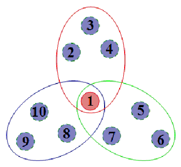
The first hypergraph is illustrated in Figure 1. There are ten vertices $V=\{1,2,\ldots,10\}$ and three edges $E=\{e_{1}=\{1,2,3,4\},e_{2}=\{1,5,6,7\},e_{3}=\{1,8,9,10\}\}$. Hence, it is a $4$-graph, and its degrees are $d(1)=3$ and $d(i)=1$ for $i=2,\ldots,10$. So we have $\Delta=3$. Moreover, this hypergraph is odd-bipartite since we could take $U=\{1\}\subset V$.

Obviously, the adjacency tensor $\mathcal{A}$ and the signless Laplacian tensor $\mathcal{Q}$ of a hypergraph $G$ are nonnegative. Moreover, they are weakly irreducible if and only if $G$ is connected [47]. Hence, we could apply the Ng-Qi-Zhou algorithms [43, 10, 59] for computing their largest H-eigenvalues and associated H-eigenvectors. On the other hand, the Laplacian tensor $\mathcal{L}$ of a uniform hypergraph $G$ is a $M$-tensor [57, 16]. Qi [49, Theorem 3.2] proved that zero is the smallest H-eigenvalue of $\mathcal{L}$. However, the following problems are still open.

• •

  How to compute the largest H-eigenvalue of $\mathcal{L}$?

• •

  How to calculate the smallest H-eigenvalues of $\mathcal{Q}$ and $\mathcal{A}$?

• •

  How to obtain extreme Z-eigenvalues of $\mathcal{A}$, $\mathcal{L}$, and $\mathcal{Q}$?

Many theorems in spectral hypergraph theory are proved to address H- and Z-eigenvalues of $\mathcal{A}$, $\mathcal{L}$, and $\mathcal{Q}$ when the involved hypergraph has well geometric structures. For convenience, we denote the largest H-eigenvalue and the smallest H-eigenvalue of a tensor $\mathcal{T}$ related to a hypergraph $G$ as $\lambda_{\max}^{H}(\mathcal{T}(G))$ and $\lambda_{\min}^{H}(\mathcal{T}(G))$ respectively. We also define similar notations for Z-eigenvalues of that tensor.

Khan and Fan [31] studied a sort of non-odd-bipartite hypergraph and gave the following result.

The adjacency tensor $\mathcal{A}$, the Laplacian tensor $\mathcal{L}$, and the signless Laplacian tensor $\mathcal{Q}$ of a uniform hypergraph are usually sparse. For instance, $\mathcal{A}$, $\mathcal{L}$ and $\mathcal{Q}$ of the $4$-uniform sunflower illustrated in Figure 1 only contain $0.72\%$, $0.76\%$, and $0.76\%$ nonzero elements respectively. Hence, it is an important issue to explore the sparsity in tensors $\mathcal{A}$, $\mathcal{L}$, and $\mathcal{Q}$ involved in a hypergraph $G$. Now, we introduce a fast numerical approach based on MATLAB.

For instance, we consider the $4$-uniform sunflower shown in Figure 1. The edge-vertex incidence matrix of this sunflower is a $3$-by-$10$ sparse matrix

From the viewpoint of scientific computing, we prefer to store the incidence matrix of the sunflower in a compact form

Obviously, the number of columns of the matrix $G_{r}$ is less than the original incidence matrix, since usually $k\ll n$. We can benefit from this compact matrix in the process of computing. In MATLAB, this matrix $G_{r}$ is written in Line 2 of Figure 2.

We first consider the degree tensor $\mathcal{D}$. It is a diagonal tensor and its $i$th diagonal element is the degree $d(i)$ of a vertex $i\in V$. Once the hypergraph $G$ is given, the degree vector ${\bf d}\equiv[d(i)]\in\mathbb{R}^{n}$ is fixed. So we could save ${\bf d}$ from the start. Let $\delta(\cdot,\cdot)$ be the Kronecker delta, i.e., $\delta(i,j)=1$ if $i=j$ and $\delta(i,j)=0$ if $i\neq j$. Using this notation, we could rewrite the degree as

To calculate the degree vector $d$ efficiently, we construct an $n$-by-$mk$ sparse matrix $M_{sp}=[\delta(i,(G_{r})_{\ell j})]$. By summarizing each row of $M_{sp}$, we obtain the degree vector ${\bf d}$. For any vector ${\bf x}\in\mathbb{R}^{n}$, the computation of

are straightforward, where “$\ast$” denotes the component-wise Hadamard product. In Figure 2, we show these codes in Lines 4-15.

Second, we focus on the adjacency tensor $\mathcal{A}$. We construct a matrix $X_{mat}=[x_{(G_{r})_{\ell j}}]$ which has the same size as $G_{r}$. Assume that the $(\ell,j)$-th element of $G_{r}$ is $i$. Then, the $(\ell,j)$-th element of $X_{mat}$ is defined as $x_{i}$. From this matrix, we rewrite the product $\mathcal{A}{\bf x}^{k}$ as

See Lines 18 and 27 of Figure 2. To compute the vector $\mathcal{A}{\bf x}^{k-1}$, we use the following representation

For each $j=1,\ldots,k$, we construct a sparse matrix $M_{j}=[\delta(i,(G_{r})_{\ell j})]\in\mathbb{R}^{n\times m}$ and a column vector ${\bf y}_{j}=[\prod_{s\neq j}(X_{mat})_{\ell s}]\in\mathbb{R}^{m}$ respectively. Then, the vector

could be computed by using a simple loop. See Lines 17-24 of Figure 2.

The computational costs for computing products of tensors $\mathcal{A}$, $\mathcal{L}$, and $\mathcal{Q}$ with any vector ${\bf x}$ are about $mk^{2}$, $mk^{2}+nk$, and $mk^{2}+nk$ multiplications, respectively. Since $mk^{2}<mk^{2}+nk\leq 2mk^{2}$, the computational cost of the product of a vector and a large scale sparse tensor related with a hypergraph is cheap. Additionally, the codes listed in Figure 2 could easily be extended to parallel computing.

The design of the novel CEST algorithm is based on a unified formula for the H- and Z-eigenvalue of a symmetric tensor [9, 17]. Let $\mathcal{I}\in\mathbb{R}^{[k,n]}$ be an identity tensor whose diagonal elements are all one and off-diagonal elements are zero. Hence, $\mathcal{I}{\bf x}^{k-1}={\bf x}^{[k-1]}$. If $k$ is even, we define $\mathcal{E}\in\mathbb{R}^{[k,n]}$ such that $\mathcal{E}{\bf x}^{k-1}=({\bf x}^{\top}{\bf x})^{\frac{k}{2}-1}{\bf x}.$ Using tensors $\mathcal{I}$ and $\mathcal{E}$, we could rewrite systems (1) and (2) as

where $\mathcal{B}=\mathcal{I}$ and $\mathcal{B}=\mathcal{E}$ respectively. In the remainder of this paper, we call a real $\lambda$ and a nonzero vector ${\bf x}\in\mathbb{R}^{n}$ an eigenvalue and its associated eigenvector respectively if they satisfies (3). Now, we devote to compute such $\lambda$ and ${\bf x}$ for large scale sparse tensors.

Let $k$ be even. We consider the spherical optimization problem

where the symmetric tensor $\mathcal{T}$ arises from a $k$-uniform hypergraph, so $\mathcal{T}$ is sparse and may be large scale. $\mathcal{B}$ is a symmetric positive definite tensor with a simple structure such as $\mathcal{I}$ and $\mathcal{E}$. Without loss of generality, we restrict ${\bf x}$ on a compact unit sphere $\mathbb{S}^{n-1}\equiv\{{\bf x}\in\mathbb{R}^{n}:{\bf x}^{\top}{\bf x}=1\}$ because $f({\bf x})$ is zero-order homogeneous.

The gradient of $f({\bf x})$ [12] is

Obviously, for all ${\bf x}\in\mathbb{S}^{n-1}$, we have

This equality implies that the vector ${\bf x}\in\mathbb{S}^{n-1}$ is perpendicular to its (negative) gradient direction. The following theorem reveals the relationship between the spherical optimization (4) and the eigenvalue problem (3).

Next, we focus on numerical approaches for computing a first-order stationary point of the spherical optimization (4). First, we apply the limited memory BFGS (L-BFGS) approach for generating a search direction. Then, a curvilinear search technique is explored to preserve iterates in a spherical constraint.

First, we prove that the sequence of merit function values $\{f({\bf x}_{c})\}$ converges and every accumulation point of iterates $\{{\bf x}_{c}\}$ is a first-order stationary point. Second, using the Kurdyka-Łojasiewicz property, we show that the sequence of iterates $\{{\bf x}_{c}\}$ is also convergent. When the second-order sufficient condition holds at the limiting point, CEST enjoys a linear convergence rate. Finally, when we start CEST from plenty of randomly initial points, resulting eigenvalues may touch the extreme eigenvalue of a tensor with a high probability.

References

- [1] Hédy Attouch and Jérôme Bolte, On the convergence of the proximal algorithm for nonsmooth functions involving analytic features, Mathematical Programming, 116 (2009), pp. 5–16.
- [2] Hédy Attouch, Jérôme Bolte, Patrick Redont, and Antoine Soubeyran, Proximal alternating minimization and projection methods for nonconvex problems: An approach based on the Kurdyka-Łojasiewicz inequality, Mathematics of Operations Research, 35 (2010), pp. 438–457.
- [3] Hedy Attouch, Jérôme Bolte, and Benar Fux Svaiter, Convergence of descent methods for semi-algebraic and tame problems: proximal algorithms, forward–backward splitting, and regularized Gauss–Seidel methods, Mathematical Programming, Series A, 137 (2013), pp. 91–129.
- [4] Jonathan Barzilai and Jonathan M. Borwein, Two-point step size gradient methods, IMA Journal of Numerical Analysis, 8 (1988), pp. 141–148.
- [5] Jérôme Bolte, Aris Daniilidis, and Adrian Lewis, The Łojasiewicz inequality for nonsmooth subanalytic functions with applications to subgradient dynamical systems, SIAM Journal on Optimization, 17 (2007), pp. 1205–1223.
- [6] Jérôme Bolte, Shoham Sabach, and Marc Teboulle, Proximal alternating linearized minimization for nonconvex and nonsmooth problems, Mathematical Programming, Series A, 146 (2014), pp. 459–494.
- [7] Changjiang Bu, Yamin Fan, and Jiang Zhou, Laplacian and signless laplacian z-eigenvalues of uniform hypergraphs, Frontiers of Mathematics in China, (2015), p. TBA.
- [8] Samuel Rota Bulo and Marcello Pelillo, New bounds on the clique number of graphs based on spectral hypergraph theory, in Learning and Intelligent Optimization, Springer, 2009, pp. 45–58.
- [9] Kung-Ching Chang, Kelly J. Pearson, and Tan Zhang, On eigenvalue problems of real symmetric tensors, Journal of Mathematical Analysis and Applications, 350 (2009), pp. 416–422.
- [10] Kung-Ching Chang, Kelly J. Pearson, and Tan Zhang, Primitivity, the convergence of the NQZ method, and the largest eigenvalue for nonnegative tensors, SIAM Journal on Matrix Analysis and Applications, 32 (2011), pp. 806–819.
- [11] Liping Chen, Lixing Han, and Liangmin Zhou, Computing tensor eigenvalues via homotopy methods, (2015). http://arxiv.org/abs/1501.04201.
- [12] Yannan Chen, Liqun Qi, and Qun Wang, Computing eigenvalues of large scale hankel tensors, Journal of Scientific Computing, (2015). DOI: 10.1007/s10915-015-0155-8.
- [13] Joshua Cooper and Aaron Dutle, Spectra of uniform hypergraphs, Linear Algebra and its Applications, 436 (2012), pp. 3268–3292.
- [14] Chun-Feng Cui, Yu-Hong Dai, and Jiawang Nie, All real eigenvalues of symmetric tensors, SIAM Journal on Matrix Analysis and Applications, 35 (2014), pp. 1582–1601.
- [15] Yu-hong Dai, A positive BB-like stepsize and an extension for symmetric linear systems, Workshop on Optimization for Modern Computation, Beijing, China, 2014. http://bicmr.pku.edu.cn/conference/opt-2014/slides/Yuhong-Dai.pdf.
- [16] Weiyang Ding, Liqun Qi, and Yimin Wei, -tensors and nonsingular -tensors, Linear Algebra and its Applications, 439 (2013), pp. 3264 – 3278.
- [17] Weiyang Ding and Yimin Wei, Generalized tensor eigenvalue problems, SIAM Journal on Matrix Analysis and Applications, 36 (2015), pp. 1073–1099.
- [18] V. A. Skorobogatov E. V. Konstantinova, Molecular structures of organoelement compounds and their representation as labeled molecular hypergraphs, Journal of Structural Chemistry, 39 (1998), pp. 268–276.
- [19] Eldar Fischer, Arie Matsliah, and Asaf Shapira, Approximate hypergraph partitioning and applications, SIAM Journal on Computing, 39 (2010), pp. 3155–3185.
- [20] S. Friedland, S. Gaubert, and L. Han, Perron-Frobenius theorem for nonnegative multilinear forms and extensions, Linear Algebra and its Applications, 438 (2013), pp. 738–749.
- [21] Yue Gao, Meng Wang, Dacheng Tao, Rongrong Ji, , and Qionghai Dai, 3-d object retrieval and recognition with hypergraph analysis, IEEE Transactions on Image Processing, 21 (2012), pp. 4290–4303.
- [22] Gourab Ghoshal, Vinko Zlatić, Guido Caldarelli, and M. E. J. Newman, Random hypergraphs and their applications, Physical Review E, 79 (2009), p. 066118.
- [23] Debarghya Ghoshdastidar and Ambedkar Dukkipati, A provable generalized tensor spectral method for uniform hypergraph partitioning, in Proceedings of The 32nd International Conference on Machine Learning, 2015, pp. 400–409.
- [24] David F. Gleich, Lek-Heng Lim, and Yongyang Yu, Multilinear pagerank, SIAM Journal on Matrix Analysis and Applications, 36 (2015), pp. 1507–1541.
- [25] Lixing Han, An unconstrained optimization approach for finding real eigenvalues of even order symmetric tensors, Numerical Algebra, Control and Optimization (NACO), 3 (2013), pp. 583–599.
- [26] Chun-Lin Hao, Chun-Feng Cui, and Yu-Hong Dai, A sequential subspace projection method for extreme Z-eigenvalues of supersymmetric tensors, Numerical Linear Algebra with Applications, 22 (2015), pp. 283–298.
- [27] Christopher J. Hillar and Lek-Heng Lim, Most tensor problems are NP-hard, Journal of the ACM, 60 (2013), pp. Article 45:1–39.
- [28] Shenglong Hu, Liqun Qi, and Jinshan Xie, The largest Laplacian and signless Laplacian H-eigenvalues of a uniform hypergraph, Linear Algebra and its Applications, 469 (2015), pp. 1–27.
- [29] George Karypis, Rajat Aggarwal, Vipin Kumar, and Shashi Shekhar, Multilevel hypergraph partitioning: applications in vlsi domain, IEEE Transactions on Very Large Scale Integration (VLSI) Systems, 7 (1999), pp. 69–79.
- [30] Enver Kayaaslan, Ali Pinar, Ümit Çatalyürek, and Cevdet Aykanat, Partitioning hypergraphs in scientific computing applications through vertex separators on graphs, SIAM Journal on Scientific Computing, 34 (2012), pp. A970–A992.
- [31] Murad-ul-Islam Khan and Yi-Zheng Fan, The H-spectrum of a generalized power hypergraph, (2015). http://arxiv.org/abs/1504.03839.
- [32] Steffen Klamt, Utz-Uwe Haus, and Fabian Theis, Hypergraphs and cellular networks, PLOS Computational Biology, 5 (2009), p. e1000385.
- [33] Tamara G. Kolda and Jackson R. Mayo, Shifted power method for computing tensor eigenpairs, SIAM Journal on Matrix Analysis and Applications, 32 (2011), pp. 1095–1124.
- [34] Tamara G. Kolda and Jackson R. Mayo, An adaptive shifted power method for computing generalized tensor eigenpairs, SIAM Journal on Matrix Analysis and Applications, 35 (2014), pp. 1563–1581.
- [35] Elena V. Konstantinova and Vladimir A. Skorobogatov, Molecular hypergraphs: The new representation of nonclassical molecular structures with polycentric delocalized bonds, Journal of Chemical Information and Computer Sciences, 35 (1995), pp. 472–478.
- [36] Jing Lei and Alessandro Rinaldo, Consistency of spectral clustering in stochastic block models, The Annals of Statistics, 43 (2015), pp. 215–237.
- [37] Xi Li, Weiming Hu, Chunhua Shen, Anthony Dick, and Zhongfei Zhang, Context-aware hypergraph construction for robust spectral clustering, IEEE Transactions on Knowledge and Data Engineering, 26 (2014), pp. 2588–2597.
- [38] Lek-Heng Lim, Singular values and eigenvalues of tensors: a variational approach, in Computational Advances in Multi-Sensor Adaptive Processing, 2005 1st IEEE International Workshop on, IEEE, 2005, pp. 129–132.
- [39] Dong C. Liu and Jorge Nocedal, On the limited memory BFGS method for large scale optimization, Mathematical Programming, 45 (1989), pp. 503–528.
- [40] Yongjun Liu, Guanglu Zhou, and Nur Fadhilah Ibrahim, An always convergent algorithm for the largest eigenvalue of an irreducible nonnegative tensor, Journal of Computational and Applied Mathematics, 235 (2010), pp. 286–292.
- [41] Stanislaw Lojasiewicz, Une propriété topologique des sous-ensembles analytiques réels, Les Équations aux Dérivées Partielles, (1963), pp. 87–89.
- [42] Tom Michoel and Bruno Nachtergaele, Alignment and integration of complex networks by hypergraph-based spectral clustering, Physical Review E, 86 (2012), p. 056111.
- [43] Michael Ng, Liqun Qi, and Guanglu Zhou, Finding the largest eigenvalue of a nonnegative tensor, SIAM Journal on Matrix Analysis and Applications, 31 (2009), pp. 1090–1099.
- [44] Qin Ni and Liqun Qi, A quadratically convergent algorithm for finding the largest eigenvalue of a nonnegative homogeneous polynomial map, Journal of Global Optimization, 61 (2015), pp. 627–641.
- [45] Jorge Nocedal, Updating quasi-newton matrices with limited storage, Mathematics of Computation, 35 (1980), pp. 773–782.
- [46] Jorge Nocedal and Stephen J. Wright, Numerical Optimization, Springer, 2006.
- [47] Kelly J. Pearson and Tan Zhang, On spectral hypergraph theory of the adjacency tensor, Graphs and Combinatorics, 30 (2014), pp. 1233–1248.
- [48] Liqun Qi, Eigenvalues of a real supersymmetric tensor, Journal of Symbolic Computation, 40 (2005), pp. 1302–1324.
- [49] Liqun Qi, -eigenvalues of Laplacian and signless Laplacian tensors, Communications in Mathematical Sciences, 12 (2014), pp. 1045–1064.
- [50] Liqun Qi, Fei Wang, and Yiju Wang, Z-eigenvalue methods for a global polynomial optimization problem, Mathematical Programming, 118 (2009), pp. 301–316.
- [51] Karl Rohe, Sourav Chatterjee, and Bin Yu, Spectral clustering and the high-dimensional stochastic blockmodel, The Annals of Statistics, (2011), pp. 1878–1915.
- [52] Jia-Yu Shao, Hai-Ying Shan, and Bao feng Wu, Some spectral properties and characterizations of connected odd-bipartite uniform hypergraphs, Linear and Multilinear Algebra, 63 (2015), pp. 2359–2372.
- [53] Wenyu Sun and Ya xiang Yuan, Optimization Theory and Methods: Nonlinear Programming, Springer, 2006.
- [54] Jinshan Xie and Liqun Qi, The clique and coclique numbers¡¯bounds based on the h-eigenvalues of uniform hypergraphs, International Journal of Numerical Analysis and Modeling, 12 (2015), pp. 318–327.
- [55] Yangyang Xu and Wotao Yin, A block coordinate descent method for regularized multiconvex optimization with applications to nonnegative tensor factorization and completion, SIAM Journal on Imaging Sciences, 6 (2013), p. 17581789.
- [56] Jun Yu, Dacheng Tao, and Meng Wang, Adaptive hypergraph learning and its application in image classification, IEEE Transactions on Image Processing, 21 (1012), pp. 3262–3272.
- [57] Liping Zhang, Liqun Qi, and Guanglu Zhou, -tensors and some applications, SIAM Journal on Matrix Analysis and Applications, 35 (2014), pp. 437–452.
- [58] Guanglu Zhou, Liqun Qi, and Soon-Yi Wu, Efficient algorithms for computing the largest eigenvalue of a nonnegative tensor, Frontiers of Mathematics in China, 8 (2013), pp. 155–168.
- [59] Guanglu Zhou, Liqun Qi, and Soon-Yi Wu, On the largest eigenvalue of a symmetric nonnegative tensor, Numerical Linear Algebra with Applications, 20 (2013), pp. 913–928.
- [60] Jason Y Zien, Martine DF Schlag, and Pak K Chan, Multilevel spectral hypergraph partitioning with arbitrary vertex sizes, IEEE Transactions on Computer-Aided Design of Integrated Circuits and Systems, 18 (1999), pp. 1389–1399.