On Delay-Optimal Scheduling in Queueing Systems with ReplicationsThanks: Yin Sun and C. Emre Koksal are with the Department of Electrical and Computer Engineering, the Ohio State University, Columbus, OH. Email: sunyin02@gmail.com, koksal.2@osu.edu. Ness B. Shroff is with the Departments of Electrical and Computer Engineering and Computer Science and Engineering, the Ohio State University, Columbus, OH. Email: shroff.11@osu.edu.
Abstract
In modern computer systems, jobs are divided into short tasks and executed in parallel. Empirical observations in practical systems suggest that the task service times are highly random and the job service time is bottlenecked by the slowest straggling task. One common solution for straggler mitigation is to replicate a task on multiple servers and wait for one replica of the task to finish early. The delay performance of replications depends heavily on the scheduling decisions of when to replicate, which servers to replicate on, and which job to serve first. So far, little is understood on how to optimize these scheduling decisions for minimizing the delay to complete the jobs. In this paper, we present a comprehensive study on delay-optimal scheduling of replications in both centralized and distributed multi-server systems. Low-complexity scheduling policies are designed and are proven to be delay-optimal or near delay-optimal in stochastic ordering among all causal and non-preemptive policies. These theoretical results are established for general system settings and delay metrics that allow for arbitrary arrival processes, arbitrary job sizes, arbitrary due times, and heterogeneous servers with data locality constraints. Novel sample-path tools are developed to prove these results.
Index Terms:
Queueing systems, replications, delay optimality, data locality, sample-path ordering, work-efficiency ordering, stochastic ordering.I Introduction
Achieving low delay is imperative in modern computer systems. Google has found that increasing the delay of Web searching from 0.4 seconds to 0.9 seconds decreases the traffic and ad revenues by 20% [1]. Similar results were reported by Amazon, where every 100 milliseconds of extra response time was shown to decrease the sales by 1% [2]. These results imply that prompt responses not only allow users to view more pages in the same period of time, but also provide instant gratification to motivate them to spend more time online [3]. In addition, low delay is critically important for the stock market, where the fastest trading decisions are made within a few milliseconds. It was estimated that a 1-millisecond advantage in trading can be worth 100 million dollars a year for a major brokerage firm [4]. Therefore, even small changes in delay can have a significant impact on business success.
As the size and complexity of computer systems continues its significant growth, maintaining low delay becomes increasingly challenging. Long-running jobs are broken into a batch of short tasks which can be executed in parallel over many servers [5]. Experience in practical systems suggests that the response times of individual servers are highly random, because of resource sharing, network congestion, cache misses, database blocking, background activities, and so on [6]. As a result, the job service delay is constrained by the slowest straggling tasks, causing a long delay tail.
An efficient technique used to tame the delay tail is replications [7, 8, 9, 10, 11, 12], which is also called redundant requests [13, 14, 15] and cloning [16, 17]. In this technique, multiple replicas of a task are dispatched to different servers and the first completed replica is considered as the valid execution of the task. After that, the remaining replicas of this task can be cancelled to release the servers, possibly with a certain amount of cancellation delay overhead. The potential benefits of replications are huge. For example, in Google’s BigTable service which has a high degree of parallelism, replications can reduce the 99.9%-th percentile delay from 1,800 milliseconds to 74 milliseconds [6]. However, in some other systems, replications may worsen the delay performance, e.g., [18, 9]. In particular, the delay performance of replications depends heavily on the scheduling decisions of when to replicate, which servers to replicate on, and which job to serve first. So far, little is understood on how to optimally schedule replications for minimizing the delay to complete the jobs.
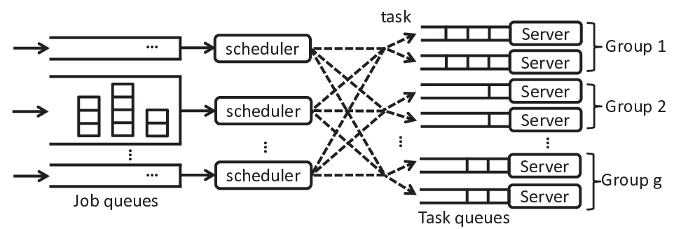
In this paper, we study delay-optimal scheduling of replications for centralized and distributed multi-server queueing systems, which are illustrated in Fig. 1 and Fig. 2, respectively. Each job brings with it a batch of tasks, and each task is of one unit of work. The jobs arrive over time according to a general arrival process, where the number, batch sizes, arrival times, and due times of the jobs are arbitrarily given. In centralized queueing systems, the jobs arrive at a scheduler and are stored in a job queue. The scheduler determines the assignment, replication, and cancellation of the tasks, based on the casual information (the history and current information) of the system. In distributed queueing systems, the jobs arrive at multiple parallel schedulers and each scheduler make decisions independently, subject to data locality constraints [19, 20]. More specifically, the servers are divided into multiple server groups, and each task can be only assigned by one group of servers, each of which stores one copy of the data necessary for executing the task.11 1 The data locality constraints considered here are hard constraints, where the servers are not allowed to process remote tasks belonging to other groups. There exists another form of soft data locality constraints, where a server can execute remote tasks belonging to other groups by first retrieving the necessary data and then processing the task. Therefore, remote tasks are executed at a slower speed than local tasks. In practical systems, hard data locality constraints are more appropriate for interactive Web services, which need to respond within a few seconds or even shorter time; while soft data locality constraints are usually used in offline services, where the tasks are executed at a slower time scale and hence there is sufficient time to retrieve the necessary data. The service times of the tasks follow New-Better-than-Used (NBU) distributions or New-Worse-than-Used (NWU) distributions, and are independent across the servers and i.i.d. across the tasks assigned to the same server. Our goal is to seek for low-complexity scheduling policies that optimize the delay performance of the jobs.

I-A Difficulty of Delay-Optimal Scheduling
Without replications, the models that we consider belong to the class of multi-class multi-server queueing systems, where delay optimality has been extremely difficult to achieve. For example, delay minimization in deterministic scheduling problems (where the service time of each job is known) with more than one servers is -hard and has no constant competitive ratio [21]. Similarly, delay-optimal stochastic scheduling (where the service time of each job is random) in multi-class multi-server queueing systems is deemed to be notoriously difficult [22, 23, 24]. Prior attempts on solving the delay-optimal scheduling problem have met little success, except in some limiting regions such as large system limits, e.g., [25], and heavy traffic limits, e.g., [26]. However, these results may not apply outside of these limiting regions or when the stationary distribution of the system does not exist.
In addition, replications add a further layer of difficulty to this problem. If a task is replicated on multiple servers, its service time is reduced, but at a cost of longer waiting times of other tasks. In general, it is difficult to determine whether the gain of shorter service time would exceed the loss of longer waiting times. Hence, “to replicate or not to replicate” is a fundamental dilemma that needs to be resolved in order to design a delay-optimal scheduler. We note that each task has many replication modes (i.e., it can be replicated on different servers and at different time instants), which require different amounts of service time. Thus, the work conservation law [27, 28] does not hold in the study of replications. Hence, certain powerful and well-known delay minimization methods, such as the achievable region approach [29, 24], are difficult to apply to our study.
I-B Summary of Main Results
We develop a number of low-complexity scheduling policies. For arbitrarily given job parameters (including the number, batch sizes, arrival times, and due times of the jobs), these policies are proven to be delay-optimal or near delay-optimal in stochastic ordering for minimizing several classes of delay metrics among all causal and non-preemptive22 2 We consider task-level non-preemptive policies: Processing of a task cannot be interrupted until the task is completed or cancelled; after completing or cancelling a task, the server can switch to process another task from any job. policies. Some examples of the delay metrics considered in this paper include the average delay, maximum delay, maximum lateness, increasing and Schur convex functions of delay (e.g., the second moment of delay), etc.33 3 To the best of our knowledge, except for the average delay, the other delay metrics are considered in the study of replications for the first time. In particular, the proposed policies are proven to be within a constant additive delay gap from the optimum for minimizing the mean average delay.
The key tools in our proofs are new sample-path orderings for comparing the delay performance of different policies. These sample-path orderings are very general because they do not need to specify the queueing system model, and hence can be potentially used for establishing near delay optimality results in other scheduling problems. The interested readers are referred to Appendix A.
I-C Organization of the Paper
We describe the model and problem formulation in Section III, together with the notations that we will use throughout the paper. Replication policies and their delay performance are analyzed for centralized queueing systems in Section IV, and for distributed queueing systems in Section V. Numerical results are provided in Section VI. Finally, the conclusion is drawn in Section VII. The sample-path proof method is provided in Appendix A.
II Related Work
II-A Systems Work
The benefits of exploiting replications to reduce delay have been empirically studied for many applications [5, 30, 31, 32, 6, 16, 17, 33, 34, 9, 35, 18, 36]. In communication networks, multiple replicated copies of a message can be sent over different routing paths to reduce delay [36, 9]. In cloud computing systems, the task execution time is highly random and it was shown that replicating straggling tasks can significantly reduce the job service delay [5, 30, 31, 32, 17, 33, 6]. In [34, 9], the authors observed that the delay of DNS queries can be reduced by sending multiple replications of a query to multiple servers.
Replications and more general coding techniques have been proposed to reduce communication delay in cloud storage and information retrieval systems. In [35, 18], the authors performed experiments on Amazon S3, and found that one can exploit storage redundancy to issue multiple downloading connections to reduce delay. Recently, coding techniques were introduced to speedup distributed algorithms such as MapReduce and machine learning [37, 38]. Significant performance improvements were shown through experiments on Amazon EC2 [38].
II-B Theoretical Work
There has been a growing interest in understanding and characterizing the delay performance of replication and coding techniques. One focus in this area is fast data retrieval in distributed storage systems. In [39], Huang et al. showed that codes can reduce the queueing delay in distributed storage systems. In [40, 41, 42], the authors obtained bounds on the mean average delay of redundant data downloading policies. In [35, 18], Liang and Kozat provided an approximate analysis for the delay performance of redundant data downloading policies, based on their measurements on Amazon S3. There also exist some analytical studies on distributed computing systems. In [11, 12], Wang et al. studied the tradeoff between delay and computing cost in cloud computing systems. For Poisson arrivals and exponential service times, Gardner et al. [14] characterized the response time distribution for several replication policies in distributed queueing systems. Recently, the delay performance of replications was analyzed in the context of load-balancing [43, 44, 45], where the number of servers may potentially grow to infinity.
In addition to the aforementioned studies that focus on delay analysis and characterization, there also exist a few works which aim to find delay-optimal scheduling policies of replications and coding. If the task service times are geometrically distributed and each job has a single task, it was shown in [46] that distributing the tasks over the servers as evenly as possible is delay-optimal among all admissible policies. Later, delay-optimal scheduling of replications was studied for more general service time distributions, such as New-Better-than-Used (NBU) distributions and New-Worse-than-Used (NWU) distributions [47, 48]. In [13, 15, 49], the delay performance of replication policies was analyzed in a few different models, where the optimal policies were obtained for minimizing the mean average delay within a specific family of policies. In [10], Chen et al. presented some similar results with [13], where the difference is that the delay optimality results in [10] were established among all admissible policies. In [50], (near) delay-optimal scheduling results were established for general maximum distance separable (MDS) codes in distributed storage systems.
This paper differs from the existing works in two aspects: First, our study is carried out for very general system settings and delay metrics, some of which are considered in the study of replications for the first time. Second, in our study, delay optimality results are established when it is possible; and in some more general scenarios where delay optimality is inherently difficult to achieve, alternative near delay optimality results with small sub-optimality gaps are obtained.
III Model and Formulation
III-A Notations and Definitions
We will use lower case letters such as and , respectively, to represent deterministic scalars and vectors. In the vector case, a subscript will index the components of a vector, such as . We use and , respectively, to denote the -th largest and the -th smallest components of . For any -dimensional vector , let denote the increasing rearrangements of . Let denote the vector with all 0 components.
Random variables and vectors will be denoted by upper case letters such as and , respectively, with the subscripts and superscripts following the same conventions as in the deterministic case. Throughout the paper, “increasing/decreasing” and “convex/concave” are used in the non-strict sense. LHS and RHS denote, respectively, “left-hand side” and “right-hand side”.
For any -dimensional vectors and , the elementwise vector ordering , , is denoted by . Further, is said to be majorized by , denoted by , if (i) , and (ii) [51]. In addition, is said to be weakly majorized by from below, denoted by , if , ; is said to be weakly majorized by from above, denoted by , if , [51]. A function that preserves the majorization order is called a Schur convex function. Specifically, is termed Schur convex if for all [51]. A function is termed symmetric if for all . The composition of functions and is denoted by . Define .
Let and denote sets and events, with denoting the cardinality of . For all random variable and events , let denote a random variable with the conditional distribution of for given . A random variable is said to be stochastically smaller than another random variable , denoted by , if for all . A set is called upper, if whenever and . A random vector is said to be stochastically smaller than another random vector , denoted by , if for all upper sets . If and , then and follow the same distribution, denoted by . We remark that if, and only if holds for all increasing provided the expectations exist [52].
A random variable is said to be smaller than another random variable in the hazard rate ordering, denoted by , if for all and all . A random variable is said to be smaller than another random variable in the increasing convex ordering, denoted by , if holds for all increasing functions provided the expectations exist [52].
III-B System Model
Consider a system with servers, which starts to operate at time . A sequence of jobs arrive at time instants , where can be either finite or infinite and . The -th incoming job, also called job , brings with it a batch of tasks. Each task is the smallest unit of work that can be assigned to a server. Job is completed when all tasks of job are completed. The maximum job size is44 4 If , then the operator in (1) is replaced by .
| (1) |
III-B1 Service Time Distributions
In practice, the service times of the tasks are highly random due to many reasons, including resource sharing, network congestion, cache misses, database blocking, etc. [6], and the servers may operate at different service speeds because they have different amounts of resources, e.g., CPU, memory, I/O bandwidth [53, 54]. Motivated by this, we assume that the task service times are independent across the servers and i.i.d. across the tasks assigned to the same server. Let be a random variable representing the task service time of server . The service rate of server is , which may vary across the servers. We consider the following classes of NBU and NWU task service time distributions.
Definition 1.
Consider a non-negative random variable with complementary cumulative distribution function (CCDF) . Then, is New-Better-than-Used (NBU) if for all
| (2) |
On the other hand, is New-Worse-than-Used (NWU) if is absolutely continuous and for all
| (3) |
NBU distributions include increasing failure rate (IFR) distributions and log-concave distributions as special cases. Examples of NBU distributions include constant service time, shifted exponential distribution, geometrical distribution, Erlang distribution, etc. Recent measurements [35, 18] show that the data downloading time in Amazon AWS can be approximated as a shifted exponential distribution. NWU distributions include the classes of decreasing failure rate (DFR) distributions and log-convex distributions. Examples of NWU distributions include hyperexponential distribution, Pareto type II (Lomax) distribution [55], gamma distributions with , Weibull distribution with , etc. In some systems [56], the task service time can be modeled as a hyperexponential distribution. A random variable is both NBU and NWU if, and only if, it is exponential.
III-B2 Queueing Models with Replications
We consider both centralized and distributed queueing models:
Centralized queueing model: In a centralized queueing system, the jobs arrive at a scheduler and are stored in a job queue, as shown in Fig. 1. A scheduler assigns tasks to the available servers over time.


In order to reduce delay, a task can be replicated on multiple servers, possibly at different time instants. The task is deemed completed as soon as one copy of the task is completed; after that, the other redundant copies of the task are either executed until completion or cancelled with a certain amount of cancellation delay overhead. We assume that the cancellation overheads are independent across the servers and i.i.d. across the tasks cancelled on the same server. Let be a random variable representing the cancellation overhead of server . Denote and , which are assumed to be mutually independent.
Distributed queueing model: In a distributed queueing system, the jobs arrive at a number of parallel schedulers, and are stored in the job queues associated to the schedulers, as depicted in Fig. 2. Each scheduler independently assigns tasks to the servers. The servers are divided into groups. Each server has a task queue, which stores the tasks assigned from different schedulers. The decisions of the schedulers are subject to data locality constraints [19, 20]. More specifically, each task can be only executed by one group of servers, each of which stores one copy of the data necessary for executing the task.
There are multiple ways to assign a task to its required group of the servers. The Power of Choices [57, 58] load balancing policy is illustrated in Fig. 3(a), where the scheduler queries the queue lengths of servers in one group, and selects the server with the shortest queue length. In this policy, it may happen that some queues in the group are empty and the other queues in the group are not, which reduces the efficiency of the system. Two alternative task assignment policies are depicted in Fig. 3(b) and Fig. 3(c), where the scheduler simultaneously places multiple copies of a task to all the servers in one group, and the servers are allowed to communicate with each other to cancel the redundant task copies. Such an approach is advocated by Google [6]. In Fig. 3(b), when one copy of a task starts execution, a message is sent to cancel the other redundant task copies. This policy is called the Cancel-After-Execution policy. In Fig. 3(c), when one copy of a task completes execution, a message is sent to cancel the other redundant task copies. This policy is called the Cancel-Before-Execution policy, which was also named “tied-requests” in [6] and “late-bindling” in [20]. It was pointed out in [6, 20] that the Cancel-Before-Execution policy can potentially achieve a better delay performance than the Power of Choices load balancing policy.


We note that each scheduling policy in Fig. 3 for distribution queueing systems has one equivalent scheduling policy for centralized queueing systems. In particular, The Power of Choices load balancing policy in Fig. 3(a) is equivalent to one instant of the Assign-When-Enqueueing policy in Fig. 4(a), the Cancel-After-Execution policy in Fig. 3(b) is equivalent to the Replication policy in Fig. 4(b), and the Cancel-Before-Execution policy in Fig. 3(c) is equivalent to the No-Replication policy in Fig. 4(c). In this paper, we will establish a unified framework to study delay-optimal scheduling of replications in centralized and distributed queueing systems.
III-C Scheduling Policies
A scheduling policy, denoted by , determines the task assignments, replications, and cancellations in the system. We consider the class of causal policies, in which scheduling decisions are made based on the history and current state of the system; the realization of task service time is unknown until the task is completed (unless the service time is deterministic). In practice, service preemption is costly and may lead to complexity and reliability issues [20, 59]. Motivated by this, we assume that task-level preemption is not allowed. Hence, if a server starts to process a task, it must complete or cancel this task before switching to process another task. We use to denote the set of causal and non-preemptive policies. Let us define several types of policies within :
A policy is said to be anticipative, if it has access to the parameters of future arriving jobs (but not other future information). For periodic and pre-planned services, future job arrivals can be predicted in advance. To cover these scenarios, we abuse the definition of causal policies a bit and include anticipative policies into the policy space . However, it should be emphasized that the policies that we propose in this paper are not anticipative.
Definition 2.
A task is termed remaining if it is either stored in the queue or being executed by the servers, and is termed unassigned if it is stored in the queue and not being executed by any server.
A policy is said to be work-conserving, if no server is idle when there are unassigned tasks waiting in the queue.
The goal of this paper is to design low-complexity non-anticipative scheduling policies that are (near) delay-optimal among all policies in , even compared to the anticipative policies with knowledge about future arriving jobs.
III-D Delay Metrics
Each job has a due time , also called due date, which is the time that job is promised to be completed [60]. Completion of a job after its due time is allowed, but then a penalty is incurred. Hence, the due time can be considered as a soft deadline.
For each job , is the job completion time, is the delay, is the lateness after the due time , and is the tardiness (or positive lateness). Define vectors , , , , , and . Let and , respectively, denote the realizations of and . All these quantities are functions of the scheduling policy .
Several important delay metrics are introduced in the following: For any policy , the average delay is defined by55 5 If , then a operator is enforced on the RHS of (4), (5), (6), and the operator in (7) and (8) is replaced by .
| (4) |
In addition, the mean square of tardiness is
| (5) |
If , becomes the mean square of delay , i.e.,
| (6) |
since for all and .
In many systems, fairness is an important aspect of the quality-of-service. We define two delay metrics related to min-max fairness. The maximum lateness is defined by
| (7) |
if , reduces to the maximum delay , i.e.,
| (8) |
In addition, two delay metrics related to proportional fairness [61] are defined by
| (9) | ||||
| (10) |
where is a positive number, which can be as small as we wish.
In general, a delay metric can be expressed as a function of the job completion times , where is increasing. In this paper, we consider three classes of delay metric functions:
For each , the delay metric is Schur convex in the lateness vector . Similarly, for each , the delay metric is Schur convex in the delay vector . Furthermore, every convex and symmetric function is Schur convex. Using these properties, we can get
III-E Delay Optimality and Its Approximation
Define as the parameters of the jobs, which include the number, batch sizes, arrival times, and due times of the jobs. The job parameters and random task service times are determined by two external processes, which are mutually independent and do not change according to the scheduling policy adopted in the system. For delay metric function and policy space , a policy is said to be delay-optimal in stochastic ordering, if one of the following conditions is satisfied:
- 1.
For all and
(11) - 2.
for all and
(12) - 3.
By the definition of stochastic ordering [52], these three conditions are equivalent. For notational simplicity, we will omit to mention that policy (or policy ) is adopted in the system as a condition of the delay performance in the rest of the paper.
In many system settings, delay optimality is extremely difficult to achieve, even with respect to some definitions of delay optimality weaker than (11). This motivated us to study whether there exist policies that can come close to delay optimality. We will show that in many scenarios, near delay optimality can be achieved in the following sense:

Define as the earliest time that all tasks of job have started service. In other words, all tasks of job are either completed or under service at time . One illustration of is provided in Fig. 5, from which it is easy to see
| (14) |
Denote , . Let and be the realizations of and , respectively. All these quantities are functions of the scheduling policy . A policy is said to be near delay-optimal in stochastic ordering, if one the following three conditions is satisfied:
- 1.
For all and
(15) - 2.
for all and
(16) - 3.
There exist many ways to approximate (11)-(13), and obtain various forms of near delay optimality. We find that the form of near delay optimality in (15)-(17) is convenient, because it is analytically provable and leads to tight sub-optimal delay gap, as we will see in the subsequent sections.
IV Replications in Centralized Queueing Systems
In this section, we provide some delay optimality and near delay optimality results for replications in centralized queueing systems. The proofs of these results will be provided in the Appendix A by using a unified sample-path method.
IV-A Average Delay and Related Delay Metrics
If the task service times are NBU and the delay metric is within (including the average delay ), we propose a class of scheduling policies called Fewest Unassigned Tasks first with Low-Priority Replication (FUT-LPR). To understand this class of policies, let us introduce some definitions:
Definition 3.
A scheduling policy is said to follow the Fewest Unassigned Task (FUT) first discipline, if each task assigned to the servers is from the job with the fewest unassigned tasks whenever the queue is not empty (there exist unassigned tasks in the queue).
Definition 4.
A scheduling policy is said to follow the Low-Priority Replication (LPR) discipline, if it is work-cons- erving and satisfies the following two principles:
- 1.
Task Replication: If the queue is not empty (there exist unassigned tasks in the queue), then no replication is allowed; otherwise, if the queue is empty (all the tasks are under service), one can replicate the tasks arbitrarily.
- 2.
Task Cancellation: If the time to cancel a task is long than the remaining service time to complete the task in hazard rate ordering, i.e., , then choose to complete the task without cancellation; otherwise, one can choose either to cancel or to complete the task.
The LPR policies offer flexible choices for task replication and cancellation operations, which are quite convenient in practice. Examples of LPR policies include the No Replication (NR) policy in which no replication is allowed at all, and the No Idleness Replication (NIR) policy which satisfies: If the queue is not empty (there exist unassigned tasks in the queue), then no replication is allowed; otherwise, if the queue is empty (all the tasks are under service), each idle server is allocated to process a replicated copy of any remaining task. Therefore, no server is idle in the NIR policy until all jobs are completed, and hence the name.
A scheduling policy belongs to the class of Fewest Unassigned Tasks first with Low-Priority Replication (FUT-LPR) policies if it simultaneously satisfies the FUT and LPR disciplines. Examples of FUT-LPR policies include the Fewest Unassigned Tasks first policy with No Idleness Replication (FUT-NIR) policy which is illustrated in Algorithm 1, and the Fewest Unassigned Tasks first policy with No Replication (FUT-NR) policy which can be obtained from Algorithm 1 by removing Steps 15-16, 20-26. The delay performance of any instance of the FUT-LPR policies is characterized in the following theorem:
Theorem 1.
If the task service times are NBU, independent across the servers, i.i.d. across the tasks assigned to the same server, then for all , , , and
| (18) |
Let us characterize the sub-optimality delay gap of the FUT-LPR policies. For mean average delay, i.e., , it follows from Theorem 1 that
| (19) |
The difference between the LHS and RHS of (19) is
| (20) |
Recall that is the number of servers, and is the number of tasks in job . At time , all tasks of job have started service. Hence, if , then job has at most incomplete tasks that are under service at time ; if , then job has at most incomplete tasks that are under service at time . Therefore, in the FUT-LPR policies, at most tasks of job are completed during the time interval . Using this and the property of NBU distributions, we can obtain
Theorem 2.
Let , and without loss of generality . If the task service times are NBU, independent across the servers, i.i.d. across the tasks assigned to the same server, then for all and
| (21) |
where is the maximum job size in (1) and .
Theorem 1 and Theorem 2 tell us that for arbitrary number, batch sizes, arrival times, and due times of the jobs, as well as arbitrary cancellation overheads of the tasks, the class of FUT-LPR policies is near delay-optimal for minimizing the mean average delay within the policy space , even compared to the anticipative policies in that can predict the parameters of future arriving jobs.
If for , then the sub-optimality delay gap of the FUT-LPR policies is of the order . As the number of servers increases, this sub-optimality delay gap is upper bounded by which is independent of .
When there are multiple servers and multiple job classes, establishing tight additive bounds on the gap from the optimal delay performance is extremely difficult and has met with little success. In [22, 23], closed-form upper bounds on the sub-optimality gaps of the Smith’s rule and the Gittin’s index rule were established for the cases that all jobs arrive at time zero. In [24, Corollary 2], the authors studied the optimal control in multi-server systems with stationary arrivals of multiple classes of jobs, and used the achievable region method to obtain an additive sub-optimality delay gap, which is of the order . The model and methodology in [22, 23, 24] are significantly different from those in this paper.
If the task service times are NWU, we propose a policy called Fewest Unassigned Tasks first with Replication (FUT-R), which simultaneously satisfies the FUT discipline and the following replication (R) discipline.
Definition 5.
A scheduling policy is said to follow the Replication (R) discipline, if it is work-conserving and satisfies the following two principles:
- 1.
Task Replication: When a task is assigned, it is replicated on all servers.
- 2.
Task Cancellation: The cancellation overhead is assumed to be zero, such that if one task copy is completed on one server, the remaining replicated copies of this task are cancelled immediately.
The FUT-R policy is described in Algorithm 2. Its delay performance is characterized as follows:
Theorem 3.
If (i) , (ii) the task service times are NWU, independent across the servers, i.i.d. across the tasks assigned to the same server, (iii) , then for all , , and
| (22) |
Proof.
See Appendix L. ∎
Hence, policy FUT-R is delay-optimal in stochastic ordering under the conditions of Theorem 3. One special case of Theorem 3 was obtained in Theorem 3.2 of [47] and Theorem 3 of [13], where each job has a single task, i.e., . We note that compared to the traditional definition of NWU distributions in reliability theory [52, p. 1], the definition in (3) has one additional condition on the absolute continuity of . This condition is introduced to ensure that the probability for any two servers to complete task executions at the same time is zero. In particular, if two servers complete task executions at the same time, it might be better to assign these two servers to process two distinct tasks than to replicate two copies of a task on these two servers. Similar phenomena were reported in [43].
If the job sizes are arbitrarily given (i.e., Condition (i) of Theorem 3 is removed), and the task service times are exponential, the delay performance of the FUT-R policy is characterized as follows.
Theorem 4.
If (i) the task service times are exponential, independent across the servers, i.i.d. across the tasks assigned to the same server, (ii) , then for all , , and
| (23) |
If , then for all
| (24) |
Hence, if for all , the sub-optimality gap of the FUT-R policy diminishes to zero at a speed of as . Note that the sub-optimal delay gaps in Theorem 2 and Theorem 4 are independent of the job parameters, and hence remain constant for any traffic load. Because exponential distribution is both NBU and NWU, Theorems 1-4 are all satisfied for exponential service time distributions.
It is important to emphasize that the FUT discipline is a nice approximation of the Shortest Remaining Processing Time (SRPT) first discipline [62, 63]: The FUT discipline utilizes the number of unassigned tasks of a job to approximate the remaining processing time of this job, and is within a small additive sub-optimality gap from the optimum for minimizing the mean average delay in the scheduling problems that we consider.
IV-B Maximum Lateness and Related Delay Metrics
Next, we consider the maximum lateness and the delay metrics in . When the task service times are NBU, we propose a class of policies named Earliest Due Date first with Low-Priority Replication (EDD-LPR), which can be obtained by combining the following EDD discipline and the LPR discipline.
Definition 6.
A scheduling policy is said to follow the Earliest Due Date (EDD) first discipline, if each task assigned to the servers is from the job with the earliest due date whenever the queue is not empty (there exist unassigned tasks in the queue).
Two instances of the EDD-LPR policies are policy Earliest Due Date first with No Idleness Replication (EDD-NIR) and policy Earliest Due Date first with No Replication (EDD-NR). Policy EDD-NIR can be obtained from Algorithm 1 by revising Step 12 as . Policy EDD-NR can be obtained by revising Step 12 of Algorithm 1 and further removing Steps 15-16, 20-26. The delay performance of policy EDD-LPR is characterized in the following theorem:
Theorem 5.
If the task service times are NBU, independent across the servers, i.i.d. across the tasks assigned to the same server, then for all , , and
| (25) |
If the job parameters satisfy certain conditions, Theorem 5 can be generalized to all delay metrics in .
Theorem 6.
If (or and ) and is replaced by any , Theorem 5 still holds.
When the task service times are NWU, we propose a policy called Earliest Due Date first with Replication (EDD-R). This policy is similar with the FUT-R policy, except that in the EDD-R policy, all servers are allocated to process replicated copies of a task from the job with the earliest due time. The EDD-R policy can be obtained from Algorithm 2 by revising Step 8 as . The delay performance of the EDD-R policy is provided as follows.
Theorem 7.
If (i) , (ii) the task service times are NWU, independent across the servers, i.i.d. across the tasks assigned to the same server, and (iii) , then for all and
| (26) |
If the jobs sizes satisfy certain conditions, Theorem 7 can be generalized to all delay metrics in .
Theorem 8.
If and is replaced by any , Theorem 7 still holds.
If the task service times are exponential, the delay performance of the EDD-R policy is characterized in the following two theorems.
Theorem 9.
If (i) the task service times are exponential, independent across the servers, i.i.d. across the tasks assigned to the same server, (ii) , then for all , and
| (27) |
Theorem 10.
If (or and ) and is replaced by any , Theorem 9 still holds.
IV-C Maximum Delay and Related Delay Metrics
Finally, we consider maximum delay and the delay metrics in . When the task service times are NBU, we propose a policy named First-Come, First-Served with Low-Priority Replication (FCFS-LPR), which can be obtained by combining the following FCFS discipline and the LPR discipline.
Definition 7.
A scheduling policy is said to follow the First-Come, First-Served (FCFS) first discipline, if each task assigned to the servers is from the job with the earliest arrival time whenever the queue is not empty (there exist unassigned tasks in the queue).
Two instances of the FCFS-LPR policies are Earliest Due Date first with No Idleness Replication (FCFS-NIR) and First-Come, First-Served with No Replication (FCFS-NR). Policy FCFS-NIR can be obtained from Algorithm 1 by revising Step 12 as . Policy FCFS-NR can be obtained by revising Step 12 of Algorithm 1 and further removing Steps 15-16, 20-26. The delay performance of FCFS-LPR is characterized as follows:
Corollary 1.
If the task service times are NBU, independent across the servers, i.i.d. across the tasks assigned to the same server, then for all , , and
| (28) |
If the job sizes satisfy certain conditions, Corollary 1 can be generalized to all delay metrics in .
Corollary 2.
If and is replaced by any , Corollary 1 still holds.
When the task service times are NWU, we propose a policy called First-Come, First-Served with Replication (FCFS-R). This policy is similar with the FUT-R policy, except that in the FCFS-R policy, all servers are allocated to process replicated copies of a task from the job with the earliest arrival time. The FCFS-R policy can be obtained from Algorithm 2 by revising Step 8 as . The delay performance of the FCFS-R policy is provided as follows.
Corollary 3.
If (i) the task service times are NWU, independent across the servers, i.i.d. across the tasks assigned to the same server, and (ii) , then for all , and
| (29) |
Corollary 4.
If and is replaced by any , Corollary 3 still hold.
Corollaries 1-4 follow directly from Theorems 5-8 by setting for all job . Nonetheless, due to the importance of the maximum delay metric and the FCFS queueing discipline, Corollaries 1-4 are of independent interests.
We note that it is difficult to obtain an additive sub-optimality delay gap for minimizing the maximum lateness or maximum delay that remains constant for any number of jobs . This is because the maximum lateness and maximum delay will likely grow to infinity as the number of jobs increases, due to the maximum operator over all jobs. Hence, unlike the average delay , the maximum lateness and maximum delay are unstable delay metrics as . In our future work, we will consider stable delay metrics and try to establish tight additive gaps from the optimal delay.
V Replications in Distributed Queueing Systems
In this section, we propose scheduling policies for replications in distributed queueing systems with data-locality constraints,66 6 Note that if there is no data-locality constraint, each task can be assigned on all servers. In this case, a distributed queueing system can be equivalently viewed as a centralized queueing system and all results in Section IV apply directly. and prove that these policies are near delay-optimal for minimizing several classes of delay metrics. To the extent of our knowledge, these are the first results on delay-optimal scheduling of replications in distributed queueing systems with data-locality constraints.
V-A An Equivalent Distributed Queueing Model
There are two types of data locality constraints: per-task constraints and per-job constraints [20]. In per-task data locality constraints, the tasks of one job may have a different group of servers on which it can run; while in per-job data locality constraints, all tasks of one job must be executed on a predetermined group of servers. Per-task constraints are more general than per-job constraints, and are also more difficult to handle. Both types of constraints play an important role in cloud computing [19]. We will consider both types of data locality constraints in our study.
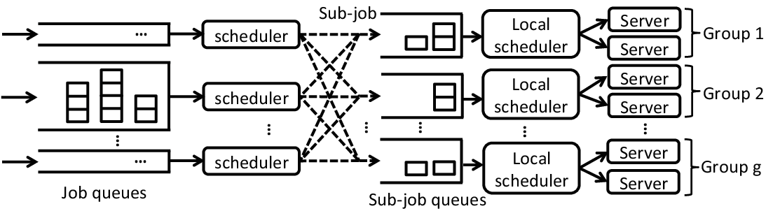
For the convenience of analysis, we consider a hierarchical distributed queueing model depicted in Fig. 6. In this model, there are two levels of job queues: the job queues at the schedulers, and the sub-job queues at the server groups. At the scheduler side, each incoming job is split into sub-jobs, where the -th sub-job consists of the tasks to be executed by server group and . Each sub-job is routed its corresponding server group, and stored in a local queue. Then, a local scheduler assigns tasks to the servers within the group. In this hierarchical distributed queueing model, each local queue for a group of servers can be considered as a centralized queueing system in Fig. 1. It is important to note that this hierarchical distributed queueing model is equivalent to the original distributed queueing model in Fig. 2. In particular, according to the discussions in Section III-B, each decision of the local scheduler in the hierarchical distributed queueing model can be equivalently implemented in the original distributed queueing model, and vice versa.
Let denote the number of tasks in -th sub-job of job , where . If no task of job should be executed by -th group of the servers, then . The arrival time and due time of each sub-job of job are and , respectively. Define as the parameters of the sub-jobs of server group . For sub-job of job , is the earliest time that all tasks of the sub-job have entered the servers, is the completion time, is the delay, and is the lateness after the due time . If , we set . Then, it holds that . In addition, a job is completed when all of its sub-jobs are completed, i.e.,
| (30) |
where and depend only on the sub-jobs with positive sizes . Define and . Let and denote the -th smallest components of and , respectively. All these quantities are functions of the adopted scheduling policy .
Note that under per-job data locality constraints, each job can be only executed by one predetermined group of the servers. Therefore, for each job there exists such that , , and for all other server groups satisfying .
Next, we will exploit the results in Section IV to study the delay performance of replications in distributed queueing systems.
V-B Per-Task Data Locality Constraints
We first consider delay minimization with per-task data locality constraints. For minimizing the maximum lateness , we propose one policy called Earliest Due Date first with Group-based Replication (EDD-GR): In the hierarchical distributed queueing model, once a job arrives at a scheduler, it is split into sub-jobs which are immediately routed to the local schedulers. If the task service times are NBU for one group of servers, the local scheduler will make decisions by following policy EDD-LPR; if the task service times are NWU for one group of servers, the local scheduler will make decisions by following policy EDD-R; if the task service times are exponential for one group of servers, the local scheduler can either choose EDD-LPR or EDD-R. According to the discussions in Section III-B, policy EDD-LPR (policy EDD-R) can be implemented in the original distributed queueing model as follows: First, replicate each task to all the local task queues in the corresponding group of servers (see Fig. 2), and then let the servers to communicate with each other to determine the replication and cancellation operations by following the LPR discipline (R discipline); each task assigned to the servers has earliest due date among all the unassigned tasks whenever the queue is not empty (there exist unassigned tasks in the queue). Hence, policy EDD-GR can be implemented distributedly. The delay performance of policy EDD-GR is provided as follows.
Theorem 11.
If (i) the task service times are independent across the servers and i.i.d. across the tasks assigned to the same server, (ii) each server group and its sub-job parameters satisfy the conditions of Theorem 5, Theorem 7, or Theorem 9, and (iii) the system is subject to per-task data locality constraints, then for all and
| (31) |
Proof.
See Appendix P. ∎
For minimizing the maximum delay , we propose one policy called First-Come, First-Served with Group-based Replication (FCFS-GR): If the task service times are NBU for one group of servers, the local scheduler will make decisions by following policy FCFS-LPR; if the task service times are NWU for one group of servers, the local scheduler will make decisions by following policy FCFS-R; if the task service times are exponential for one group of servers, the local scheduler can either choose FCFS-LPR or FCFS-R. Similar with policy EDD-GR, policy FCFS-GR can also be implemented distributedly in the original distributed queueing systems. By choosing for all , it follows from Theorem 11 that
Corollary 5.
If (i) the task service times are independent across the servers and i.i.d. across the tasks assigned to the same server, (ii) each server group and its sub-job parameters satisfy the conditions of Corollary 1 or Corollary 3, and (iii) the system is subject to per-task data locality constraints, then for all and
| (32) |
V-C Per-Job Data Locality Constraints
It is difficult for us to generalize Theorem 11 and Corollary 5 and minimize other delay metrics under per-task data locality constraints. However, under per-job data locality constraints such generalizations are possible, which are discussed in the sequel.
For minimizing the delay metrics in (including the average delay ), we propose one policy called Fewest Unassigned Tasks first with Group-based Replication (FUT-GR): If the task service times are NBU for one group of servers, the local scheduler will make decisions by following policy FUT-LPR; if the task service times are NWU for one group of servers, the local scheduler will make decisions by following policy FUT-R; if the task service times are exponential for one group of servers, the local scheduler can either choose FUT-LPR or FUT-R. Hence, the priority of a sub-job is determined by the number of unassigned tasks in this sub-job. The delay performance of policy FUT-GR is provided as follows.
Theorem 12.
If (i) the task service times are independent across the servers and i.i.d. across the tasks assigned to the same server, (ii) each server group and its sub-job parameters satisfy the conditions of Theorem 1, Theorem 3, or Theorem 4, and (iii) the system is subject to per-job data locality constraints, then for all , , and
| (33) |
Proof.
See Appendix Q. ∎
Let us further consider the delay metrics in the set , for which we can obtain the following result.
Theorem 13.
If (i) the task service times are independent across the servers and i.i.d. across the tasks assigned to the same server, (ii) each server group and its sub-job parameters satisfy the conditions of Theorem 6, Theorem 8, or Theorem 10, and (iii) the system is subject to per-job data locality constraints, then for all , , and
| (34) |
Proof.
See Appendix R. ∎
Finally, if for all job , it follows from Theorem 13 that
Corollary 6.
If (i) the task service times are independent across the servers and i.i.d. across the tasks assigned to the same server, (ii) each server group and its sub-job parameters satisfy the conditions of Corollary 2 or Corollary 4, and (iii) the system is subject to per-job data locality constraints, then for all , , and
| (35) |
VI Numerical Results
In this section, we present some numerical results to illustrate the delay performance of different scheduling policies and validate our theoretical results.
VI-A Centralized Queueing Systems
Consider a centralized queueing system consisting of 3 servers with heterogeneous service time distributions, The inter-arrival time of the jobs is exponentially distributed for even ; and is zero for odd . Let be the average job arrival rate.

VI-A1 Average Delay
Figure 7 plots the expected average delay versus traffic intensity in a centralized queueing system with heterogeneous NWU service time distributions. The number of incoming jobs is , the job size is chosen to be either or with equal probability. The task service time follows a shifted exponential distribution:
and the service rate of the 3 servers are , , and , respectively. The traffic intensity can be computed as . The cancellation overhead of server is exponentially distributed with rate . The “Lower bound” curve is generated by using which, according to Theorem 1, is a lower bound of the optimum expected average delay. We can observe from Fig. 7 that the policies FCFS-NR, FUT-NR, and FUT-NIR are throughput-optimal, while the policies FCFS-R and FUT-R have a smaller throughput region. The average delays of policies FUT-NR and FUT-NIR are quite close to the lower bound, while the other policies are far from the lower bound.

Figure 8 illustrates the expected average delay versus traffic intensity in a centralized queueing system with heterogeneous NWU service time distributions. The number of incoming jobs is , the job sizes are for all . The task service time follows a Pareto type II (Lomax) distribution [68]:
| (38) |
where , , , and . The cancellation overhead is zero for all servers. According to the property of Pareto type II (Lomax) distribution [68], the maximum task service rate is , which is achieved when each task is replicated on all 3 servers. Hence, the traffic intensity can be computed as . Because all jobs are of the same size, the FUT discipline is identical with the FCFS discipline. We can observe that policy FUT-R, which is identical with policy FCFS-R, is throughput-optimal, while policy FUT-NR and policy FUT-NIR have a smaller throughput region. In addition, policy FUT-R achieves better delay performance than the other policies, which is in accordance with Theorem 3.

Figure 9 depicts the expected average delay versus traffic intensity in a centralized queueing system with heterogeneous exponential service time distributions. The number of incoming jobs is , the job size is chosen to be either or with equal probability. The service rate of the 3 servers are , , and , respectively. The cancellation overhead is zero for all servers. The maximum task service rate is . Hence, the traffic intensity can be computed as . The “Lower bound” curve is generated by using which, according to Theorem 1, is a lower bound of the optimum expected average delay. We can observe that the delay performance of policy FUT-R is close to the lower bound, compared with the other policies.

VI-A2 Maximum Lateness
Figure 10 evaluates the complementary CDF of maximum lateness versus in a centralized queueing system with heterogeneous NBU service time distributions. The number of incoming jobs is , the job size is chosen to be either or with equal probability, and the due time is chosen to be either or with equal probability. The distributions of task service times and cancellation overheads are the same with those in Fig. 7. The traffic intensity is set as . The “Lower bound” curve is generated by using , which, according to Theorem 5, is a lower bound of the optimum delay performance. We can observe that the complementary CDF of the maximum lateness of policies EDD-NR and EDD-NIR are close to the lower bound curve. In addition, the delay performance of policy FCFS-NR is better than that of FCFS-R and EDD-R. This is because policy FCFS-NR has a larger throughput region than policy FCFS-R and policy EDD-R.

Figure 11 shows the complementary CDF of maximum lateness versus for a centralized queueing system with heterogeneous NWU service time distributions. The number of incoming jobs is , the job size is chosen to be either or with equal probability, and the due time is . The distributions of task service times and cancellation overheads are the same with those in Fig. 8. The traffic intensity is set as . Because , the EDD discipline is identical with the FCFS discipline. We can observe that policy EDD-R, which is identical with policy FCFS-R, achieves better performance than the other policies, which is in accordance with Theorem 7.

Figure 12 provides the complementary CDF of maximum lateness versus for a centralized queueing system with heterogeneous exponential service time distributions. The number of incoming jobs is , the job size is chosen to be either or with equal probability, and the due time is chosen to be either or with equal probability. The distributions of task service times and cancellation overheads are the same with those in Fig. 9. The traffic intensity is set as . The “Lower bound” curve is generated by using . We can observe that the delay performance of policy EDD-R is quite close to the lower bound curve. The delay performance of policy EDD-NR and policy EDD-NIR is a bit farther than from the lower bound curve. Policy FCFS-R and policy FCFS-NR have the worse performance. These results are in accordance with Theorem 5 and Theorem 9.


VI-A3 Maximum Delay
Figure 13 plots the complementary CDF of maximum delay versus in a centralized queueing system with heterogeneous NBU service time distributions. The system model is the same with that of Fig. 10. The “Lower bound” curve is generated by using , which, according to Corollary 1, is a lower bound of the optimum delay performance. We can observe that the delay performance of policy FCFS-NR and policy FCFS-NIR is close to the lower bound curve. In addition, the delay performance of policy EDD-NR is better than that of FCFS-R and EDD-R because policy EDD-NR has a larger throughput region than policy FCFS-R and policy EDD-R.
Figure 14 illustrates the complementary CDF of maximum delay versus in a centralized queueing system with heterogeneous NWU service time distributions. The system model is almost the same with that of Fig. 11, except that the due time is chosen to be either or with equal probability. We can observe that the delay performance of policy FCFS-R is much better than that of the other policies, which validates Corollary 3.


VI-B Some Other Delay Metrics
Figure 15 shows the root mean square of tardiness versus traffic intensity in a centralized queueing system with heterogeneous NBU service time distributions, where
The system model is similar with that of Fig. 13, except that for all job and the due time is either or with equal probability. The “Lower bound” curve is generated by using , which, according to Theorem 6, is a lower bound of the optimum delay performance. We can observe that the delay performance of policy EDD-NR and policy EDD-NIR is close to the lower bound curve, and is better than that of the other policies. Notice that as , policy EDD-R and policy EDD-NIR tends become the same policy, and hence has the same delay performance.
Figure 16 presents the root mean square of tardiness versus traffic intensity in a centralized queueing system with heterogeneous exponential service time distributions. The system model is similar with that of Fig. 14, except that for all job and the due time is either or with equal probability. The “Lower bound” curve is generated by using , which, according to Theorem 10, is a lower bound of the optimum delay performance. We can observe that the delay performance of policy EDD-R is close to the lower bound curve, and is better than that of the other policies.


Figure 17 illustrates the root mean square of delay versus traffic intensity in a centralized queueing system with heterogeneous NBU service time distributions, where
The system model is almost the same with that of Fig. 13, except that for all job . The “Lower bound” curve is generated by using , which, according to Corollary 2, is a lower bound of the optimum delay performance. We can observe that the delay performance of policy FCFS-NR and policy FCFS-NIR is close to the lower bound curve, and is much better than the other policies.
Figure 18 presents the root mean square of delay versus traffic intensity in a centralized queueing system with heterogeneous NWU service time distributions. The system model is almost the same with that of Fig. 14, except that for all job . We can observe that the delay performance of policy FCFS-R is much better than that of the other policies, which validates Corollary 4.

VI-C Distributed Queueing Systems
Next, we provide some numerical results for the delay performance of replications in distributed queueing systems with data locality constraints. The inter-arrival time of the jobs is exponentially distributed for even ; and is zero for odd . The number of incoming jobs is . The due time of job is or with equal probability. The traffic intensity is set as .
Figure 19 evaluates the complementary CDF of maximum lateness versus in a distributed queueing system with per-task data locality constraints. The system has groups of servers, each consisting of 3 servers. The size of each sub-job is or with equal probability. The distributions of task service times and cancellation overheads of one group of servers are the same with those in Fig. 7, and the distributions of task service times and cancellation overheads of the other group of servers are the same with those in Fig. 9. The “Lower bound” curve is generated by using , which, according to Theorem 11, is a lower bound of the optimum delay performance. We can observe that The delay performance of policy EDD-GR is close to the lower bound curve. In addition, policy EDD-NR and EDD-GR have similar performance. This is because exponential distribution is also NBU. Hence, both groups of servers have NBU service time distributions.

Figure 20 depicts the complementary CDF of maximum delay versus in a distributed queueing system with per-task data locality constraints. This system has groups of servers, each consisting of 3 servers. The size of each sub-job is or with equal probability. The distributions of task service times and cancellation overheads of two groups of servers are the same with those in Fig. 19, and the distributions of task service times and cancellation overheads of the third group of servers are the same with those in Fig. 8. The “Lower bound” curve is generated by using , which, according to Corollary 5, is a lower bound of the optimum delay performance. We can see that the delay performance of policy FCFS-GR is quite close to the lower bound curve and is much better than that of the other policies.
VII Conclusion
This paper presented a comprehensive study on delay-optimal scheduling of batch jobs with replications in multi-server systems. A number of low-complexity scheduling policies are developed and are proven to be (near) delay-optimal in a stochastic ordering sense for minimizing three general classes of delay metrics among all causal and non-preemptive policies. The key tools in our proofs are new sample-path conditions for comparing the delay performance of different policies. These sample-path conditions do not need to specify the queueing system model and hence can potentially be applied to obtain (near) delay-optimal results for other scheduling systems. An interesting topic for future research is to develop an analytical framework to design (near) delay-optimal scheduling of replications and coding under general service time distributions (that go beyond NBU and NWU). In addition, service time correlation across the servers has significant influence on the delay performance of replications and coding, which requires further investigation.
Appendix A Sample-path Method
We propose a unified sample-path method to prove the theorems in Section IV. This method contains three steps:
- 1.
Sample-path Orderings: We first introduce several sample-path orderings (Propositions 1-4 and Corollaries 7-8). Each of these sample-path orderings can be used to obtain a delay inequality for comparing the delay performance (i.e., average delay, maximum lateness, or maximum delay) of different policies.
- 2.
Sufficient Conditions for Sample-path Orderings: As we have mentioned, each task has many replication modes, which require different amounts of service time. In order to minimize delay, the scheduler needs to choose efficient replication modes to execute the tasks as fast as possible. Motivated by this, we introduce two work-efficiency orderings to compare the efficiency of task executions in different policies. By combining these work-efficiency orderings with appropriate priority rules (i.e., FUT, EDD, FCFS) for job services, we obtain several sufficient conditions (Propositions 5-8) of the sample-path orderings in Step 1. In addition, if more than one sufficient conditions are simultaneously satisfied, we are able to obtain delay inequalities for comparing more general classes of delay metrics achieved by different policies (Propositions 9-12).
- 3.
Coupling Arguments: We use coupling arguments to prove that for NBU and NWU task service times and appropriate replication rules, the work-efficiency orderings are satisfied in the sense of stochastic ordering (Lemmas 1-3). By combining this with the priority rules (i.e., FUT, EDD, FCFS), we are able to prove the sufficient conditions in Step 2 in the sense of stochastic ordering. By this, the main results of this paper are proven.
This sample-path method is quite general. In particular, Step 1 and Step 2 do not need to specify the queueing system model, and can be potentially used for establishing (near) delay optimality results in other systems.
A-A Step 1: Sample-path Orderings
We first propose several sample-path orderings to compare the delay performance of different scheduling policies. Let us first define the system state of any policy .
Definition 8.
At any time instant , the system state of policy is specified by a pair of -dimensional vectors and with non-negative components, where is the total number of jobs and can be either finite or infinite. The components of and are interpreted as follows: If job is present in the system at time , then is the number of remaining tasks (which are either stored in the queue or being executed by the servers) of job , and is the number of unassigned tasks (which are stored in the queue and not being executed by any server) of job ; if job is not present in the system at time (i.e., job has not arrived at the system or has departed from the system), then . Hence, for all , , and
| (39) |
Let denote the state process of policy in a probability space , which is assumed to be right-continuous. The realization of the state process on a sample path can be expressed as . To ease the notational burden, we will omit henceforth and reuse to denote the realization of the state process on a sample path. Because the system starts to operate at time , there is no job in the system before time . Hence, .
The following proposition provides one condition (40) for comparing the average delay of different policies on a sample path, which was firstly introduced in [63] to prove the optimality of the preemptive SRPT policy for minimizing the average delay in single-server scheduling problems.
Proposition 1.
For any given job parameters and a sample path of two policies , if 77 7 In majorization theory [51], (40) is equivalent to “ is weakly supermajorized by , i.e., ”.
| (40) |
holds for all , where is the -th largest component of , then
| (41) |
where is the -th smallest component of .88 8 In other words, is the earliest time in policy by which jobs have been completed in policy . Hence,
| (42) |
Proof.
Suppose that there are unfinished jobs at time in policy , then . By (40), we get and hence there are at most unfinished jobs in policy . In other words, there are at least as many unfinished jobs in policy as in policy at any time . This implies (41), because the sequence of job arrival times are invariant under any policy. In addition, (42) follows from (41), which completes the proof. ∎
The sample-path ordering (40) is quite insightful. According to Proposition 1, if (40) holds for all policies and all sample paths , then policy is sample-path delay-optimal for minimizing the average delay . Interestingly, Proposition 1 is also necessary: If (40) does not hold at some time , then one can construct an arrival process after time such that (41) and (42) do not hold [63].
The sample-path ordering (40) has been successfully used in single-server scheduling problems [63]. However, it cannot be directly applied in multi-server scheduling problems. In the sequel, we consider an alternative method to relax the sample-path ordering (40) and seek for near delay optimality.
Proposition 2.
For any given job parameters and a sample path of two policies , if
| (43) |
holds for all , where is the -th largest component of , then
| (44) |
where is the -th smallest component of .99 9 In other words, is the earliest time in policy that there exist jobs whose tasks have all started service. Hence,
| (45) |
Proof.
See Appendix B. ∎
Hence, by relaxing the sample-path ordering (40) as (43), a relaxed delay inequality (45) is obtained which can be used to compare the average delay of policy and policy in a near-optimal sense.
Similarly, two sample-path orderings are developed in the following two lemmas to compare the maximum lateness achieved by different policies.
Proposition 3.
For any given job parameters and a sample path of two policies , if
| (46) |
holds for all , then
| (47) |
Proof.
See Appendix C. ∎
Proposition 4.
For any given job parameters and a sample path of two policies , if
| (48) |
holds for all , then
| (49) |
Proof.
See Appendix C. ∎
If for all , the maximum lateness reduces to the maximum delay . Hence, we can obtain
Corollary 7.
For any given job parameters and a sample path of two policies , if
| (50) |
holds for all , then
| (51) |
Corollary 8.
For any given job parameters and a sample path of two policies , if
| (52) |
holds for all , then
| (53) |
The proofs of Corollary 7 and Corollary 8 are omitted, because they follow directly from Proposition 3 and Proposition 4 by setting for all . Nonetheless, due to the importance of the maximum delay metric, Corollary 7 and Corollary 8 are of independent interests.
The sample-path orderings in Propositions 1-4 and Corollaries 7-8 are of similar forms. Their distinct features are
- •
- •
- •
These features are tightly related to the priority rules for minimizing the corresponding delay metrics: The priority rule for minimizing the average delay is FUT first; the priority rule for minimizing the maximum lateness is EDD first; the priority rule for minimizing the maximum delay is FCFS. Hence, the summations in these sample-path orderings are taken over the high priority jobs. This is the key insight behind these sample-path orderings.
A number of popular sample-path methods — such as forward induction, backward induction, and interchange arguments [64] — have been successfully used to establish delay optimality results in single-server scheduling problems [62, 65, 66]. However, it is challenging to directly generalize these methods and characterize the sub-optimal delay gap from the optimum when delay optimality is essentially difficult to achieve. On the other hand, the sample-path orderings (40), (43), (46), (48), (50), and (52) provide an interesting unified framework for sample-path delay comparisons towards both delay optimality and near delay optimality. To the best of our knowledge, except for (40) developed in [63], the sample-path orderings (43), (46), (48), (50), and (52) have not appeared before.
A-B Step 2: Sufficient Conditions for Sample-path Orderings
In Step 2, we will introduce several sufficient conditions for the sample-path orderings (40), (43), (46), (48), (50), and (52). In addition, we will also develop sample-path sufficient conditions for comparing more general delay metrics in , , and .
A-B1 Work-efficiency Orderings
In traditional queueing systems without replications, the service delay is largely governed by the work conservation law (or its generalizations): At any time, the expected total amount of time for completing the jobs in the queue is invariant among all work-conserving policies [27, 28, 29]. However, this work conservation law does not hold in queueing systems with replications. In particular, each task has many replication modes (i.e., it can be replicated on different sets of servers and at different time instants), which require different amounts of service time. In order to minimize delay, the scheduler needs to choose efficient replication modes to execute the tasks. Motivated by this, we introduce an ordering to compare the efficiency of task executions in different policies. We call it work-efficiency ordering.
Let denote the total number of tasks of all jobs. Define as the sequence of task completion times in policy where . Let denote the realization of on a sample path.
Definition 9.
Work-Efficiency Ordering: For given job parameters and a sample path of two policies , policy is said to be more work-efficient than policy , if
| (54) |
The key idea of this work-efficiency ordering is to complete tasks as early as possible. This idea was used to study delay-optimal replications in [46, 47, 48] where each job has a single task, i.e., .
In some scenarios, the above work-efficiency ordering is not satisfied, but it is possible to establish the following alternative form of work-efficiency ordering:

Definition 10.
Weak Work-efficiency Ordering: For any given job parameters and a sample path of two policies , policy is said to be weakly more work-efficient than policy , if the following assertion is true: For each task executed in policy , if
- 1.
In policy , task starts service at time and completes service at time (),
- 2.
In policy , the queue is not empty (there exist unassigned tasks in the queue) during ,
then there exists one corresponding task in policy which starts service during .
An illustration of this weak work-efficiency ordering is provided in Fig. 21. Notice that this weak work-efficient ordering requires the service starting time of task in policy to be within the service duration of its corresponding task in policy . This is a key feature that will be used later to establish near delay optimality.
We note that the weak work-efficiency ordering does not follow from the work-efficiency ordering. We say it is weak in the sense that work-efficiency ordering can be used to establish delay optimality, while weak work-efficiency ordering can be used to establish near delay optimality.
A-B2 Sufficient Conditions for Sample-path Orderings
Using these two work-efficiency orderings, we can obtain the following sufficient conditions for the sample-path ordering (40) and (43) associated to the average delay .
Proposition 5.
Proof.
See Appendix D. ∎
Proposition 6.
Proof.
See Appendix E. ∎
Similarly, two sufficient conditions are obtained for the sample-path orderings (46) and (48) for comparing the maximum lateness of different policies.
Proposition 7.
Proof.
See Appendix F. ∎
Proposition 8.
Proof.
See Appendix G. ∎
A-B3 More General Delay Metrics
We now investigate more general delay metrics in and . First, Proposition 5 and Proposition 6 can be directly generalized to all delay metrics in .
Proposition 9.
If the conditions of Proposition 5 are satisfied, then for all
Proof.
See Appendix H. ∎
Proposition 10.
If the conditions of Proposition 6 are satisfied, then for all
Proof.
See Appendix H. ∎
If policy simultaneously satisfies the sufficient conditions in Proposition 5 and Proposition 7 (or Proposition 6 and Proposition 8), we can obtain a couple of delay inequalities for comparing any delay metric in .
Proposition 11.
Proof sketch of Proposition 11.
For any , (41) and (55) follow from Proposition 5 and Proposition 9. For any , we construct an -dimensional vector and show that
| (56) |
where the first majorization ordering in (56) follows from the rearrangement inequality [51, Theorem 6.F.14],[67], and the second inequality in (56) is proven by using (41). This further implies
| (57) |
Using this, we can show that (55) holds for all . The details are provided in Appendix I. ∎
Proposition 12.
Proof.
See Appendix J. ∎
A-C Step 3: Coupling Arguments
A-C1 Coupling Lemmas
We need the following three coupling lemmas to prove our main results.
Lemma 1.
Consider policy and any policy . If (i) policy follows the LPR discipline, (ii) the task service times are NBU, independent across the servers, and i.i.d. across the tasks assigned to the same server, then there exist policy and policy satisfying the same queueing disciplines with policy and policy , respectively, such that
- 1.
The state process of policy has the same distribution with the state process of policy ,
- 2.
The state process of policy has the same distribution with the state process of policy ,
- 3.
Policy is weakly more work-efficient than policy with probability one.
Proof.
See Appendix K. ∎
Lemma 2.
Consider policy and any policy . If (i) policy follows the R discipline, (ii) the task service times are NWU, independent across the servers, and i.i.d. across the tasks assigned to the same server, and (iii) the cancellation overhead is , then there exist policy and policy satisfying the same queueing disciplines with policy and policy , respectively, such that
- 1.
The state process of policy has the same distribution with the state process of policy ,
- 2.
The state process of policy has the same distribution with the state process of policy ,
- 3.
Policy is more work-efficient than policy with probability one.
Proof.
See Appendix L. ∎
Lemma 3.
Consider policy and any policy . If (i) policy follows the R discipline, (ii) the task service times are exponential, independent across the servers, and i.i.d. across the tasks assigned to the same server, and (iii) the cancellation overhead is , then there exist policy and policy satisfying the same queueing disciplines with policy and policy , respectively, such that
- 1.
The state process of policy has the same distribution with the state process of policy ,
- 2.
The state process of policy has the same distribution with the state process of policy ,
- 3.
Policy is weakly more work-efficient than policy with probability one.
Proof.
See Appendix M. ∎
We note that Theorem 6.B.3 in [52] plays an important role in the proofs of Lemmas 1-3: Because the task service times are independent across the servers and i.i.d. across the tasks assigned to the same server, we only need the NBU/NWU assumption and Theorem 6.B.3 in [52], instead of invoking the stronger likelihood ratio ordering as in [67], [52, Theorem 6.B.15], to prove these coupling lemmas.
A-C2 Proofs of the Main Results
Now, we are ready to prove the main results.
Proof of Theorem 1.
According to lemma 1, for any policy , there exist two state processes and of policy FUT-LPR1 and policy , such that (i) the state process of policy FUT-LPR1 has the same distribution with the state process of policy FUT-LPR, (ii) the state process of policy has the same distribution with the state process of policy , and (iii) policy FUT-LPR1 is weakly more work-efficient than policy with probability one.
Proof of Theorem 3.
According to lemma 2, for any policy , there exist two state processes and of policy FUT-R1 and policy , such that (i) the state process of policy FUT-R1 has the same distribution with the state process of policy FUT-R, (ii) the state process of policy has the same distribution with the state process of policy , and (iii) policy FUT-R1 is more work-efficient than policy with probability one.
In policy FUT-R1, each task completing service is from the job with the fewest remaining tasks among all jobs with remaining tasks. By (iii) and Proposition 9, for all
By (i), has the same distribution with . By (ii), has the same distribution with . Then, by the property of stochastic ordering [52, Theorem 1.A.1], we can obtain (22). This completes the proof. ∎
Proof of Theorem 4.
According to lemma 3, for any policy , there exist two state processes and of policy FUT-R1 and policy , such that (i) the state process of policy FUT-R1 has the same distribution with the state process of policy FUT-R, (ii) the state process of policy has the same distribution with the state process of policy , and (iii) policy FUT-R1 is weakly more work-efficient than policy with probability one.
Proof of Theorem 5.
Proof of Theorem 6.
If , each job has only one task. Hence, the job with the earliest due time among all jobs with unassigned tasks is also one job with the fewest unassigned tasks.
If , , in policy EDD-LPR, each task starting service is from the job with the earliest due time among all jobs with unassigned tasks, which is also the job with the fewest unassigned tasks among all jobs with unassigned tasks.
Proof of Theorem 7.
Proof of Theorem 8.
If , , in policy EDD-R, each task completing service is from the job with the earliest due time among all jobs with remaining tasks, which is also the job with the fewest remaining tasks among all jobs with remaining tasks.
Proof of Theorem 9.
Proof of Theorem 10.
If , each job has only one task. Hence, the job with the earliest due time among all jobs with unassigned tasks is also one job with the fewest unassigned tasks.
If , , in policy EDD-R, each task starting service is from the job with the earliest due time among all jobs with unassigned tasks, which is also the job with the fewest unassigned tasks among all jobs with unassigned tasks.
Appendix B Proof of Proposition 2
Let be any integer chosen from , and be the number of jobs that have arrived by the time , where . Because jobs are completed by the time in policy , there are exactly incomplete jobs in the system at time . By the definition of the system state, we have for . Hence,
Combining this with (43), yields that policy satisfies
| (59) |
Next, the definition of the system state tells us that holds for all and . Hence, we have
| (60) |
Therefore, there are at most jobs which have unassigned tasks at time in policy . Because the sequence of job arrival times are invariant under any policy, jobs have arrived by the time in policy . Thus, there are at least jobs which have no unassigned tasks at the time in policy , which can be equivalently expressed as
| (61) |
Because is arbitrarily chosen, (61) holds for all , which is exactly (44). In addition, (45) follows from (44), which completes the proof.
Appendix C Proofs of Propositions 3-4
Proof of Proposition 3.
Let be the index of the job associated with the job completion time . In order to prove (47), it is sufficient to show that for each ,
| (62) |
We prove (62) by contradiction. For this, let us assume that
| (63) |
holds for all job satisfying and . That is, if job arrives before time and its due time is no later than , then job is completed before time in policy . Define
| (64) |
According to (63) and (64), we can obtain
| (65) |
On the other hand, (64) tells us that all job satisfying and are completed by time in policy . By this, the system state of policy satisfies
Combining this with (46), yields
| (66) |
Further, the definition of the system state tells us that for all and . Using this and (66), we get that job satisfies
That is, all tasks of job are completed by time in policy . Hence, , where contradicts with (65). Therefore, there exists at least one job satisfying the conditions , , and . This can be equivalently expressed as
| (67) |
Hence, for each ,
Appendix D Proof of Proposition 5
The following two lemmas are needed to prove Proposition 5:
Lemma 4.
Lemma 5.
[63, Lemma 3] Suppose that, under policy , is obtained by adding a job with tasks to the system whose state is . Further, suppose that, under policy , is obtained by adding a job with tasks to the system whose state is . If
then
Proof of Proposition 5.
Because policy is more work-efficient than policy , the sequence of task completion times in policy are smaller than those in policy , i.e.,
| (69) |
We modify the task completion times on the sample-path of policy as follows: For each , if a task of job is completed at time on the original sample-path of policy , then on the modified sample-path of policy , the same task of job is completed at time . This modification satisfies the following three claims:
- 1.
According to (69), the task completion times of policy are postponed after the modification;
- 2.
The order of completed tasks in policy remains the same before and after the modification;
- 3.
The task completion times on the sample-path of policy and on the modified sample-path of policy are identical.
Let and denote the system state on the modified sample-path of policy . From Claims 1 and 2, we can get for all and . Therefore, for all
| (70) |
Next, we compare policy with the modified sample-path of policy . According to Claim 1, Claim 2, and , each task completing service on the modified sample-path of policy is still from the job with the fewest remaining tasks among all jobs with remaining tasks. That is, Condition 3 of Proposition 5 is satisfied on the modified sample-path of policy , which is required by Lemma 4.
Appendix E Proof of Proposition 6
The following two lemmas are needed to prove Proposition 6:
Lemma 6.
Suppose that under policy , is obtained by allocating unassigned tasks to the servers in the system whose state is . Further, suppose that under policy , is obtained by completing tasks in the system whose state is . If , condition 2 of Proposition 6 is satisfied in policy , and
then
| (72) |
Proof.
If , then the inequality (72) follows naturally. If , then there exist unassigned tasks which have not been assigned to any server. In policy , each task allocated to the servers is from the job with the minimum positive . Hence, . ∎
Lemma 7.
Suppose that, under policy , is obtained by adding a job with tasks to the system whose state is . Further, suppose that, under policy , is obtained by adding a job with tasks to the system whose state is . If
then
Proof.
Without loss of generalization, we suppose that after the job arrival, is the -th largest component of and the -th largest component of , i.e., . We consider the following four cases:
Case 1: . We have .
Case 2: . We have .
Case 3: . We have .
Case 4: . We have . ∎
Proof of Proposition 6.

Assume that no task is completed at the job arrival times for . This does not lose any generality, because if a task is completed at time , Proposition 6 can be proven by first proving for the case and then taking the limit . We prove (43) by induction.
Step 1: We will show that (43) holds during .1010 10 Note that .
Because , (43) holds at time . Job 1 arrives at time . By Lemma 7, (43) holds at time . Let be an arbitrarily chosen time during . Suppose that tasks start execution and also complete execution during in policy . We need to consider two cases:
Case 1: The queue is not empty (there exist unassigned tasks in the queue) during in policy . By the weak work-efficiency ordering condition, no fewer than tasks start execution during in policy . Because (43) holds at time , by Lemma 6, (43) also holds at time .
Case 2: The queue is empty (all tasks in the system are in service) by time in policy . Because and there is no task arrival during , there is no task arrival during . Hence, it must hold that all tasks in the system are in service at time . Then, the system state of policy satisfies for all at time . Hence, (43) holds at time .
In summary of these two cases, (43) holds for all .
Step 2: Assume that for some integer , the conditions of Proposition 6 imply that (43) holds for all . We will prove that the conditions of Proposition 6 imply that (43) holds for all .
Let be an arbitrarily chosen time during . We modify the task completion times in policy as follows: For each pair of corresponding task and task mentioned in the definition of the weak work-efficiency ordering, if
- •
In policy , task starts execution at time and completes execution at time ,
- •
In policy , the queue is not empty (there exist unassigned tasks in the queue) during ,
- •
In policy , the corresponding task starts execution at time ,
then the completion time of task is modified from to in policy , as illustrated in Fig. 22.
This modification satisfies the following three claims:
- 1.
The system state of policy at time remains the same before and after this modification;
- 2.
Policy is still weakly more work-efficient than policy after this modification;
- 3.
If tasks complete execution during on the modified sample path of policy , and the queue is not empty (there exist unassigned tasks in the queue) during in policy , then no fewer than tasks start execution during in policy .
We now prove these three claims. Claim 1 follows from the fact that the tasks completed during remain the same before and after this modification. It is easy to prove Claim 2 by checking the definition of work-efficiency ordering. For Claim 3, notice that if a task starts execution and completes execution during on the modified sample path of policy , then by Claim 2, its corresponding task must start execution during in policy . On the other hand, if a task starts execution during and completes execution during on the modified sample path of policy , then by the modification, its corresponding task must start execution during in policy . By combining these two cases, Claim 3 follows.
We use these three claims to prove the statement of Step 2. According to Claim 2, policy is weakly more work-efficient than policy after the modification. By the assumption of Step 2, (43) holds during for the modified sample path of policy . Job arrives at time . By Lemma 7, (43) holds at time for the modified sample path of policy . Suppose that tasks complete execution during on the modified sample path of policy . We need to consider two cases:
Case 1: The queue is not empty (there exist unassigned tasks in the queue) during in policy . By Claim 3, no fewer than tasks start execution during in policy . Because (43) holds at time , by Lemma 6, (43) also holds at time for the modified sample path of policy .
Case 2: The queue is empty (all tasks in the system are in service) at time in policy . Because and , there is no task arrival during . Hence, it must hold that all tasks in the system are in service at time . Then, the system state of policy satisfies for all at time . Hence, (43) holds at time for the modified sample path of policy .
In summary of these two cases, (43) holds at time for the modified sample path of policy . By Claim 1, the system state of policy at time remains the same before and after this modification. Hence, (43) holds at time for the original sample path of policy . Therefore, if the assumption of Step 2 is true, then (43) holds for all .
Appendix F Proof of Proposition 7
The proof of Proposition 7 requires the following two lemmas:
Lemma 8.
Suppose that, in policy , is obtained by completing tasks in the system whose state is . Further, suppose that, in policy , is obtained by completing tasks in the system whose state is . If , condition 3 of Proposition 7 is satisfied in policy , and
then
| (73) |
Proof.
If , then the inequality (74) follows naturally. If , then there exist some remaining tasks. In policy , each task completing service is from the job with the earliest due time. Hence, . ∎
Lemma 9.
Suppose that under policy , is obtained by adding a job with tasks and due time to the system whose state is . Further, suppose that under policy , is obtained by adding a job with tasks and due time to the system whose state is . If
then
Proof.
If , then .
If , then . ∎
Appendix G Proof of Proposition 8
The proof of Proposition 8 requires the following two lemmas:
Lemma 10.
Suppose that, in policy , is obtained by allocating unassigned tasks to the servers in the system whose state is . Further, suppose that, in policy , is obtained by completing tasks in the system whose state is . If , condition 2 of Proposition 8 is satisfied in policy , and
then
| (74) |
Proof.
If , then the inequality (74) follows naturally. If , then there exist some unassigned tasks in the queue. In policy , each task allocated to the servers is from the job with the earliest due time. Hence, . ∎
Lemma 11.
Suppose that under policy , is obtained by adding a job with tasks and due time to the system whose state is . Further, suppose that under policy , is obtained by adding a job with tasks and due time to the system whose state is . If
then
Proof.
If , then .
If , then . ∎
Appendix H Proofs of Propositions 9-10
Proof of Proposition 9.
Appendix I Proof of Proposition 11
In the proof of Proposition 11, we need to use the following rearrangement inequality:
Lemma 12.
[51, Theorem 6.F.14] Consider two -dimensional vectors and . If for two indices and where , then
Proof of Proposition 11.
For , (55) is proven in 3 steps, which are described as follows:
Step 1: We will show that
| (75) |
According to Eq. (1.A.17) and Theorem 5.A.9 of [51], it is sufficient to show that there exists an -dimensional vector such that
| (76) |
Vector is constructed as follows: First, is a rearrangement (or permutation) of the vector , which can be equivalently expressed as
| (77) |
Second, for each , if the completion time of job is the -th smallest component of , i.e.,
| (78) |
then associated with job is the -th smallest component of , i.e.,
| (79) |
Combining (41) and (77)-(79), yields
for . This implies , and hence the second inequality in (76) is proven.
The remaining task is to prove the first inequality in (76). First, consider the case that the due times of the jobs are different from each other. The vector can be obtained from by the following procedure: For each , define a set
| (80) |
If there exists two jobs and which satisfy and , we interchange the components and in vector . Repeat this interchange operation, until such two jobs and satisfying and cannot be found. Therefore, at the end of this procedure, if job arrives before and job has an earlier due time than job , then , which is satisfied by policy . Therefore, the vector is obtained at the end of this procedure. In each interchange operation of this procedure, is satisfied before the interchange of and . By Lemma 12 and the transitivity of the ordering of majorization, we can obtain , which is the first inequality in (76).
Next, consider the case that two jobs and have identical due time . Hence, . In this case, the service order of job and job are indeterminate in policy . Nonetheless, by Lemma 12, the service order of job and job does not affect the first inequality in (76). Hence, the first inequality in (76) holds even when .
Appendix J Proof of Proposition 12
For , (58) is proven in 3 steps, which are described as follows:
Step 1: We will show that
| (81) |
According to Eq. (1.A.17) and Theorem 5.A.9 of [51], it is sufficient to show that there exists an -dimensional vector such that
| (82) |
Vector is constructed as follows: First, the components of the vector is a rearrangement (or permutation) of the components of the vector , which can be equivalently expressed as
| (83) |
Second, for each , if the completion time of job is the -th smallest component of , i.e.,
| (84) |
then associated with job is the -th smallest component of , i.e.,
| (85) |
Combining (44) and (83)-(85), yields
for . This implies , and hence the second inequality in (82) is proven.
The remaining task is to prove the first inequality in (82). First, consider the case that the due times of the jobs are different from each other. The vector can be obtained from by the following procedure: For each , define a set
| (86) |
If there exist two jobs and which satisfy and , we interchange the components and in vector . Repeat this interchange operation, until such two jobs and satisfying and cannot be found. Therefore, at the end of this procedure, if job arrives before and job has an earlier due time than job , then , which is exactly the priority rule of job service satisfied by policy . Therefore, the vector is obtained at the end of this procedure. In each interchange operation of this procedure, is satisfied before the interchange of and . By Lemma 12 and the transitivity of the ordering of majorization, we can obtain , which is the first inequality in (82).
Next, consider the case that two jobs and have identical due time . Hence, . In this case, the service order of job and job are indeterminate in policy . Nonetheless, by Lemma 12, the service order of job and job does not affect the first inequality in (82). Hence, the first inequality in (82) holds even when .
Step 3: We use (81) to prove Proposition 12. For any , is increasing and Schur convex. According to Theorem 3.A.8 of [51], for all , we have
This completes the proof.

Appendix K Proof of Lemma 1
We will need the following lemma:
Lemma 13.
Suppose that are non-negative independent random variables, are arbitrarily given non-negative constants, for , then are mutually independent.
Proof.
For all constants , , we have
| (87) |
Hence, are mutually independent. ∎
Proof of Lemma 1.
We use coupling to prove Lemma 1: We construct two policies and such that policy satisfies the same queueing discipline with policy , and policy satisfies the same queueing discipline with policy . Hence, policy is work-conserving. The task and job completion times of policy (policy ) have the same distribution with those of policy (policy ). Because the state process is determined by the job parameters and the task/job completion events, the state process of policy has the same distribution with the state process of policy , and the state process of policy has the same distribution with the state process of policy .
Next, we show that policy and policy can be constructed such that policy is weakly more work-efficient than policy with probability one. Let us consider any task executed in policy . As illustrated in Fig. 23, suppose that copies of task are replicated on the servers at the time instants in policy , where .1111 11 If , there is no replication. In addition, suppose that server will complete processingits copy of task at time if there is no cancellation. Then, one of these servers will complete one copy of task at time , which is the earliest among these servers. Hence, task starts service at time and completes service at time in policy . Suppose that the queue is not empty (there exist unassigned tasks) during in policy 1. Because policy 1 is work-conserving, all servers are busy during in policy 1. In policy , let be the earliest time that server becomes available to process a new task after time . We will show that policy can be constructed such that for all ,
| (88) |
holds with probability one. Let denote the task service time of server and denote the cancellation delay overhead of server . We need to consider three cases:
Case 1: In policy , server is processing task at time , and will keep processing task until it completes task at time . Suppose that server has spent () seconds on task by time in policy 1. Then, the CCDF of is given by
| (89) |
Because the task service times are NBU, we can obtain that for all
| (90) |
By combining (89) and (90), we obtain
| (91) |
By Theorem 1.A.1 of [52], policy can be constructed such that (88) always holds in Case 1.
Case 2: In policy , server is processing task at time and will keep processing task until another server completes a copy of task ; then server will cancel its redundant copy of task and will complete the cancellation operation at time . Suppose that server has spent () seconds on processing task by time in policy 1. In addition, suppose that server will spend an additional () seconds on processing task after time in policy 1, before starting to cancel task . Then,
| (92) |
where the cancellation delay overhead of server .
First, let us consider the case that task is not cancelled. Suppose that in this case, server will complete processing task at time . As shown in Case 1, the service of task can be constructed such that
| (93) |
always holds.
Second, in Case 2, task is cancelled at . According to the LPR discipline, task cancellation only happen when the time to cancel the task is shorter than the remaining service time to complete the task in the hazard rate ordering. Hence, for all
By Theorem 1.A.1 of [52], policy can be constructed such that
| (94) |
always holds. By combining (92)-(94), policy can be constructed such that (88) always holds in Case 2.
Case 3: In policy , server is cancelling a redundant copy of task at time , and will complete the cancellation operation at time . Suppose that in policy 1, server has spent () seconds on processing task before starting to cancel task , and server has spent () seconds on cancelling task by time . Hence, for all
| (95) |
According to the LPR discipline, task cancellation only happen when the time to cancel the task is shorter than the remaining service time to complete the task in the hazard rate ordering. Hence, for all
| (96) |
Finally, because the task service times are NBU, for all
| (97) |
By combining (95)-(97), (91) follows. By Theorem 1.A.1 of [52], policy can be constructed such that (88) always holds in Case 3.
By Lemma 13, are mutually independent. Hence, policy can be constructed such that (88) holds for all with probability one. Therefore, in policy 1 there exists at least one of the server , say server , that completes processing or cancelling a task and becomes available to process a new task before time . Let denote the time that server becomes available to process a new task in policy . Because server is kept busy during , a new task, say task , will start execution on server at time in policy . Since the queue is not empty (there exist unassigned tasks in the queue) during , according to the LPR discipline, task cannot be a replicated copy of a task that has been assigned to some server before time . Hence, task starts service at time .
In the above coupling arguments, conditioned on every possible realization of policy and policy before the service of task starts, we can construct the service of task in policy and the service of the corresponding task in policy such that the requirement of weak work-efficiency ordering is satisfied for this pair of tasks. Next, following the proof of [52, Theorem 6.B.3], one can continue this procedure to progressively construct the service of all tasks in policy and policy . By this, we obtain that policy 1 is weakly more work-efficient than policy with probability one, which completes the proof. ∎
Appendix L Proof of Lemma 2
Define as the sequence of task arrival times where . Hence, is unique determined by the job arrival times and job sizes which are included in the job parameters . Recall that is the sequence of task completion times in policy where . We will show that for all
| (98) |
We prove (98) by using Theorem 6.B.3 of [52]. Consider the first task completion time . Job 1 arrives at time . Note that any policy is non-preemptive. If policy is work-conserving, then
otherwise, if policy is non-work-conserving, then
because of the possibility of server idleness. Since policy is work-conserving, we can obtain that for all
| (99) |
Next, consider the evolution from to . For any work-conserving policy , we can obtain
| (100) |
where is the remaining service time for server to complete the task being executed at time .
Because the task service times are independent across the servers and the CCDF is absolutely continuous, the probability for any two servers to complete their tasks at the same time is zero. Therefore, in policy , when a task copy is completed on a server, the remaining replicated copies of this task are still being processed on the other servers; these replicated task copies are cancelled immediately and replicated copies of a new task are assigned to the servers. Suppose that server has spent () seconds on processing a task by time in policy . Then, in policy , for . Hence, CCDF of is given by
| (101) |
If is a work-conserving policy, then we have for . Hence, Hence, CCDF of is given by
| (102) |
Because the task service times are independent NWU, by (101) and (102), for
According to Lemma 13, are mutual independent. Hence, using Theorem 6.B.16(b) of [52], yields
| (103) |
Combining (100), (103), and the fact that is uniquely determined by , it follows that for all work-conserving policy
| (104) |
If policy is non-work-conserving, (100) becomes
because of the possibility of server idleness. In this case, (104) still holds. Hence, (104) holds for all . Then, substituting (99) and (104) into Theorem 6.B.3 of [52], yields
Hence, (98) is proven. According to Theorem 6.B.1 of [52], this is equivalent to Lemma 2. This completes the proof.
Appendix M Proof of Lemma 3
We use coupling to prove Lemma 3: We construct two policies and such that policy satisfies the same queueing discipline with policy , and policy satisfies the same queueing discipline with policy . Hence, policy is work-conserving. The task and job completion times of policy (policy ) have the same distribution with those of policy (policy ). Because the state process is determined by the job parameters and the task/job completion events, the state process of policy has the same distribution with the state process of policy , and the state process of policy has the same distribution with the state process of policy .
Next, we show that policy and policy can be constructed such that policy is weakly more work-efficient than policy with probability one. Let us consider any task executed in policy . As illustrated in the upper part of Fig. 23, suppose that copies of task are replicated on the servers at the time instants in policy , where .1212 12 If , there is no replication. In addition, suppose that server will complete processingits copy of task at time if there is no cancellation. Then, one of these servers will complete one copy of task at time , which is the earliest among these servers. Hence, task starts service at time and completes service at time in policy . Suppose that the queue is not empty (there exist unassigned tasks) during in policy 1, we will show that policy 1 can be constructed such that there exists one corresponding task which starts service during .
Because policy 1 is work-conserving and there exist unassigned tasks at any time during , all servers are busy during in policy 1. Suppose that in policy , is the earliest time that one task is completed on server after time . Let denote the task service time of server which follows an exponential distribution. Because exponential distributions are memoryless, follows the same exponential distribution, i.e.,
| (105) |
Because the task service times are independent across the servers, by Lemma 13, are mutually independent. By Theorem 6.B.16(b) of [52], we can obtain
| (106) |
In policy , server starts to process task at time for , until one of the servers , say server , completes task at time . According to (105), (106), and Theorem 1.A.1 of [52], policy 1 and can be coupled such that in policy 1, server completes a task exactly at time . Since the queue is not empty (there exist unassigned tasks in the queue) during , according to the R discipline, replicated copies of a new task, say task , will be assigned to the servers at time . Hence, task starts service at time .
In the above coupling arguments, conditioned on every possible realization of policy and policy before the service of task starts in policy , we can construct the service of task in policy and the service of the corresponding task in policy such that the requirement of weak work-efficiency ordering is satisfied for this pair of tasks. Next, following the proof of [52, Theorem 6.B.3], one can continue the above procedure to progressively construct the service of all tasks in policy and policy . By this, we obtain that policy 1 is weakly more work-efficient than policy with probability one, which completes the proof.
Appendix N Proof of Theorem 2
Let us consider . At time , all tasks of job are completed or under service. if , then job has at most incomplete tasks that are under service at time ; if , then job has at most incomplete tasks that are under service at time . Therefore, in policy FUT-LPR, no more than tasks of job are completed during the time interval .
Suppose that at time , a set of servers are processing the tasks of job , which satisfies and there is no replications in the set of servers . Note that if some servers in are processing the replicated task copies of job , the delay gap that we will obtain will be even smaller.
Let denote the amount of time that server has spent on executing a task of job by time in policy FUT-LPR. Let denote the remaining service time of server for executing this task after time . Then, can be expressed as . Because the ’s are independent NBU random variables with mean , for all realizations of
In addition, Theorem 3.A.55 of [52] tells us that
where is the increasing convex order defined in [52, Chapter 4] and the ’s are independent exponential random variables with mean . Hence,
Lemma 13 tells us that the ’s are conditional independent for any given realization of . Hence, by Corollary 4.A.16 of [52], for all realizations of and
| (107) |
Then,
| (108) | ||||
| (109) | ||||
| (110) |
where (108) is due to (107) and Eq. (4.A.1) of [52], (109) is due to , , and the fact that is independent of , and (110) is due to the property of exponential distributions. Because and are random variables which are determined by the job parameters , taking the conditional expectation for given in (110), yields
By taking the average over all jobs, the first inequality of (21) is proven. In addition, it is known that for each
By this, the second inequality of (21) holds. This completes the proof.
Appendix O Proof of (22)
Consider the time difference . In policy FUT-R, all servers are allocated to process replicated copies of a task from the job with the fewest unassigned tasks. Hence, at time , one task of job are being processed by all servers. Because the ’s are independent exponential random variables with mean , by Theorem 3.A.55 of [52], we can obtain
| (111) | ||||
| (112) | ||||
| (113) |
where (111) is because one task of job are being processed by all servers at time , (112) is because is independent of , and (113) is due to the property of exponential distributions. By this, (24) is proven.
Appendix P Proof of Theorem 11
Appendix Q Proof of Theorem 12
For any policy , suppose that policy FUT-GR1 (policy ) satisfies the same queueing discipline with policy FUT-GR (policy ). By the proof arguments of Theorems 1-4 and the fact that , policy FUT-GR1 and policy can be coupled such that
| (114) |
holds with probability one for and . Under per-job data locality constraints, for each job there exists such that , , and for all . By this and (114), we can obtain
holds with probability one for . Then, Because any is a symmetric and increasing function, we can obtain
holds with probability one. Then, by the property of stochastic ordering [52, Theorem 1.A.1], we can obtain (33). This completes the proof.
Appendix R Proof of Theorem 13
If each server group and its sub-job parameters satisfy the conditions of Theorem 6, Theorem 8, or Theorem 10, then we can obtain
- 1.
The job with the earliest due time among all jobs with unassigned tasks is also the jobs with fewest unassigned tasks,
- 2.
Next, we consider the delay metrics in . For any policy , suppose that policy EDD-GR1 (policy ) satisfies the same queueing discipline with policy EDD-GR (policy ). By using the proof arguments of Theorem 6, Theorem 8, and Theorem 10, and the fact that , policy EDD-GR1 and policy can be coupled such that
holds with probability one for each . Then, Theorem 5.A.7 of [51] tells us that
| (115) |
holds with probability one. Under per-job data locality constraints, for each job there exists such that , , and for all . By this and (115), we get that
holds with probability one. In addition, by Theorem 3.A.8 of [51],
holds with probability one for all . Then, by the property of stochastic ordering [52, Theorem 1.A.1], we can obtain (34). This completes the proof.
References
- [1] G. Linden, http://glinden.blogspot.com/2006/11/marissa-mayer-at-web-20.html/.
- [2] ——, “Make data useful,” http://www.gduchamp.com/media/StanfordDataMining.2006-11-28.pdf, Stanford CS345 Talk, 2006.
- [3] D. Farber, http://www.zdnet.com/article/googles-marissa-mayer-speed-wins/.
- [4] R. Martin, http://www.informationweek.com/wall-streets-quest-to-process-data-at-the-speed-of-light/d/d-id/1054287?
- [5] J. Dean and S. Ghemawat, “MapReduce: Simplified data processing on large clusters,” in USENIX OSDI, Dec. 2004, pp. 137–150.
- [6] J. Dean and L. A. Barroso, “The tail at scale,” Commun. ACM, vol. 56, no. 2, pp. 74–80, Feb. 2013.
- [7] G. D. Ghare and S. T. Leutenegger, “Improving speedup and response times by replicating parallel programs on a SNOW,” in JSSPP, 2004.
- [8] W. Cirne, F. Brasileiro, D. Paranhos, L. W. Goes, and W. Voorsluys, “On the efficacy, efficiency and emergent behavior of task replication in large distributed systems,” Parallel Computing, vol. 33, no. 3, pp. 213 – 234, 2007.
- [9] A. Vulimiri, P. B. Godfrey, R. Mittal, J. Sherry, S. Ratnasamy, and S. Shenker, “Low latency via redundancy,” in ACM CoNEXT, 2013.
- [10] S. Chen, Y. Sun, U. Kozat, L. Huang, P. Sinha, G. Liang, X. Liu, and N. B. Shroff, “When queueing meets coding: Optimal-latency data retrieving scheme in storage clouds,” in IEEE INFOCOM, 2014.
- [11] D. Wang, G. Joshi, and G. Wornell, “Efficient task replication for fast response times in parallel computation,” in ACM Sigmetrics, 2014.
- [12] ——, “Using straggler replication to reduce latency in large-scale parallel computing,” in ACM SIGMETRICS Workshop on Distributed Cloud Computing, 2015.
- [13] N. B. Shah, K. Lee, and K. Ramchandran, “When do redundant requests reduce latency?” in Allerton Conference, 2013.
- [14] K. Gardner, S. Zbarsky, S. Doroudi, M. Harchol-Balter, E. Hyytiä, and A. Scheller-Wolf, “Queueing with redundant requests: First exact analysis,” in ACM Sigmetrics, 2015.
- [15] K. Lee, R. Pedarsani, and K. Ramchandran, “On scheduling redundant requests with cancellation overheads,” in Allerton Conference, 2015.
- [16] G. Ananthanarayanan, A. Ghodsi, S. Shenker, and I. Stoica, “Why let resources idle? aggressive cloning of jobs with dolly,” in USENIX HotCloud, 2011.
- [17] ——, “Effective straggler mitigation: Attack of the clones,” in USENIX NSDI, 2013.
- [18] G. Liang and U. Kozat, “TOFEC: Achieving optimal throughput-delay trade-off of cloud storage using erasure codes,” in IEEE INFOCOM, 2014.
- [19] V. Chudnovsky, R. Rifaat, J. Hellerstein, B. Sharma, and C. Das, “Modeling and synthesizing task placement constraints in google compute clusters,” in Symposium on Cloud Computing, 2011.
- [20] K. Ousterhout, P. Wendell, M. Zaharia, and I. Stoica, “Sparrow: Distributed, low latency scheduling,” in ACM SOSP, 2013, pp. 69–84.
- [21] S. Leonardi and D. Raz, “Approximating total flow time on parallel machines,” in ACM STOC, 1997.
- [22] G. Weiss, “Turnpike optimality of Smith’s rule in parallel machines stochastic scheduling,” Math. Oper. Res., vol. 17, no. 2, pp. 255–270, May 1992.
- [23] ——, “On almost optimal priority rules for preemptive scheduling of stochastic jobs on parallel machines,” Advances in Applied Probability, vol. 27, no. 3, pp. 821–839, 1995.
- [24] M. Dacre, K. Glazebrook, and J. Niño-Mora, “The achievable region approach to the optimal control of stochastic systems,” Journal of the Royal Statistical Society: Series B (Statistical Methodology), vol. 61, no. 4, pp. 747–791, 1999.
- [25] L. Ying, R. Srikant, and X. Kang, “The power of slightly more than one sample in randomized load balancing,” in IEEE INFOCOM, 2015.
- [26] A. L. Stolyar, “Maxweight scheduling in a generalized switch: State space collapse and workload minimization in heavy traffic,” The Annals of Applied Probability, vol. 14, no. 1, pp. 1–53, 2004.
- [27] L. Kleinrock, Queueing Systems. John Wiley and Sons, 1975, vol. 1& 2.
- [28] J. Nino-Mora, “Conservation laws and related applications,” in Wiley Encyclopedia of Operations Research and Management Science. John Wiley & Sons, Inc., 2010.
- [29] J. C. Gittins, K. Glazebrook, and R. Weber, Multi-armed Bandit Allocation Indices, 2nd ed. Wiley, Chichester, NY, 2011.
- [30] M. Zaharia, A. Konwinski, A. D. Joseph, R. Katz, and I. Stoica, “Improving MapReduce performance in heterogeneous environments,” in USENIX OSDI, 2008.
- [31] G. Ananthanarayanan, S. Kandula, A. Greenberg, I. Stoica, Y. Lu, B. Saha, and E. Harris, “Reining in the outliers in map-reduce clusters using Mantri,” in USENIX OSDI, 2010.
- [32] S. Melnik, A. Gubarev, J. J. Long, G. Romer, S. Shivakumar, M. Tolton, and T. Vassilakis, “Dremel: Interactive analysis of web-scale datasets,” in VLDB, 2010.
- [33] G. Ananthanarayanan, M. C.-C. Hung, X. Ren, I. Stoica, A. Wierman, and M. Yu, “GRASS: Trimming stragglers in approximation analytics,” in USENIX NSDI, 2014.
- [34] A. Vulimiri, O. Michel, P. B. Godfrey, and S. Shenker, “More is less: Reducing latency via redundancy,” in ACM HotNets, 2012.
- [35] G. Liang and U. Kozat, “FAST CLOUD: Pushing the envelope on delay performance of cloud storage with coding,” IEEE/ACM Trans. Networking, Dec. 2014.
- [36] S. Jain, M. Demmer, R. Patra, and K. Fall, “Using redundancy to cope with failures in a delay tolerant network,” in ACM SIGCOMM, 2005.
- [37] S. Li, M. A. Maddah-Ali, and A. S. Avestimehr, “Coded MapReduce,” in Allerton Conference, 2015.
- [38] K. Lee, M. Lam, R. Pedarsani, D. Papailiopoulos, and K. Ramchandran, “Speeding up distributed machine learning using codes,” in NIPS workshop on Machine Learning Systems, 2015.
- [39] L. Huang, S. Pawar, H. Zhang, and K. Ramchandran, “Codes can reduce queueing delay in data centers,” in IEEE ISIT, 2012.
- [40] G. Joshi, Y. Liu, and E. Soljanin, “On the delay-storage trade-off in content download from coded distributed storage systems,” IEEE J. Sel. Areas Commun., vol. 32, pp. 989–997, May 2014.
- [41] N. B. Shah, K. Lee, and K. Ramchandran, “The MDS queue: Analysing latency performance of codes,” in IEEE ISIT, 2014.
- [42] A. Kumar, R. Tandon, and T. C. Clancy, “On the latency of erasure-coded cloud storage systems,” 2014. [Online]. Available: http://arxiv.org/abs/1405.2833
- [43] B. Li, A. Ramamoorthy, and R. Srikant, “Mean-field-analysis of coding versus replication in cloud storage systems,” in IEEE INFOCOM, 2016.
- [44] K. Gardner, S. Zbarsky, M. Harchol-Balter, and A. Scheller-Wolf, “The power of d choices for redundancy,” in ACM Sigmetrics, 2016.
- [45] K. Gardner, M. Harchol-Balter, and A. Scheller-Wolf, “A better model for job redundancy: Decoupling server slowdown and job size,” in IEEE MASCOTS, Sept 2016, pp. 1–10.
- [46] S. Borst, O. Boxma, J. Groote, and S. Mauw, “Task allocation in a multi-server system,” Journal of Scheduling, vol. 6, no. 5, pp. 423–436, 2003.
- [47] G. Koole and R. Righter, “Resource allocation in grid computing,” Journal of Scheduling, vol. 11, no. 3, pp. 163–173, 2008.
- [48] Y. Kim, R. Righter, and R. Wolff, “Grid scheduling with NBU service times,” Operations Research Letters, vol. 38, no. 6, pp. 502 – 504, 2010.
- [49] G. Joshi, E. Soljanin, and G. Wornell, “Efficient redundancy techniques for latency reduction in cloud systems,” http://arxiv.org/abs/1508.03599, 2015.
- [50] Y. Sun, Z. Zheng, C. E. Koksal, K.-H. Kim, and N. B. Shroff, “Provably delay efficient data retrieving in storage clouds,” in IEEE INFOCOM, 2015.
- [51] A. W. Marshall, I. Olkin, and B. C. Arnold, Inequalities: Theory of Majorization and Its Applications, 2nd ed. Springer, 2011.
- [52] M. Shaked and J. G. Shanthikumar, Stochastic Orders. Springer, 2007.
- [53] C. Reiss, A. Tumanov, G. R. Ganger, R. H. Katz, and M. A. Kozuch, “Heterogeneity and dynamicity of clouds at scale: Google trace analysis,” in ACM SoCC, 2012.
- [54] L. Suresh, M. Canini, S. Schmid, and A. Feldmann, “C3: Cutting tail latency in cloud data stores via adaptive replica selection,” in USENIX NSDI, Oakland, CA, May 2015, pp. 513–527.
- [55] B. Arnold, E. Castillo, and J. M. Sarabia, Conditional Specifications of Statistical Models. Springer-Verlag New York, Inc., 1999.
- [56] K. Christodoulopoulos, V. Gkamas, and E. Varvarigos, “Statistical analysis and modeling of jobs in a grid environment,” Journal of Grid Computing, vol. 6, no. 1, pp. 77–101, 2008.
- [57] M. Mitzenmacher, “The power of two choices in randomized load balancing,” IEEE Transactions on Parallel and Distributed Systems, vol. 12, no. 10, pp. 1094–1104, 2001.
- [58] N. D. Vvedenskaya, R. L. Dobrushin, and F. I. Karpelevich, “Queueing system with selection of the shortest of two queues: An asymptotic approach,” Problemy Peredachi Informatsii, vol. 32, no. 1, pp. 20–34, 1996.
- [59] A. Verma, L. Pedrosa, M. R. Korupolu, D. Oppenheimer, E. Tune, and J. Wilkes, “Large-scale cluster management at Google with Borg,” in EuroSys, Bordeaux, France, 2015.
- [60] M. L. Pinedo, Scheduling: Theory, Algorithms, and Systems, 4th ed. Springer, 2012.
- [61] H. J. Kushner and P. A. Whiting, “Convergence of proportional-fair sharing algorithms under general conditions,” IEEE Transactions on Wireless Communications, vol. 3, no. 4, pp. 1250–1259, July 2004.
- [62] L. Schrage, “A proof of the optimality of the shortest remaining processing time discipline,” Operations Research, vol. 16, pp. 687–690, 1968.
- [63] D. R. Smith, “A new proof of the optimality of the shortest remaining processing time discipline,” Operations Research, vol. 16, pp. 197–199, 1978.
- [64] Z. Liu, P. Nain, and D. Towsley, “Sample path methods in the control of queues,” Queueing Systems, vol. 21, no. 3, pp. 293–335.
- [65] J. R. Jackson, “Scheduling a production line to minimize maximum tardiness,” management Science Research Report, University of California, Los Angeles, CA, 1955.
- [66] F. Baccelli, Z. Liu, and D. Towsley, “Extremal scheduling of parallel processing with and without real-time constraints,” J. ACM, vol. 40, no. 5, pp. 1209–1237, Nov. 1993.
- [67] C.-S. Chang and D. D. Yao, “Rearrangement, majorization and stochastic scheduling,” Math. of Oper. Res, 1993.
- [68] B. C. Arnold, “Pareto and generalized pareto distributions,” in Modeling Income Distributions and Lorenz Curves, ser. Economic Studies in Equality, Social Exclusion and Well-Being, D. Chotikapanich, Ed. Springer New York, 2008, vol. 5, pp. 119–145.