Putting Peer Prediction Under the Micro(economic)scope and
Making Truth-telling Focal
Abstract
Peer-prediction [18] is a (meta-)mechanism which, given any proper scoring rule, produces a mechanism to elicit privately-held, non-verifiable information from self-interested agents. Formally, truth-telling is a strict Nash equilibrium of the mechanism. Unfortunately, there may be other equilibria as well (including uninformative equilibria where all players simply report the same fixed signal, regardless of their true signal) and, typically, the truth-telling equilibrium does not have the highest expected payoff. The main result of this paper is to show that, in the symmetric binary setting, by tweaking peer-prediction, in part by carefully selecting the proper scoring rule it is based on, we can make the truth-telling equilibrium focal—that is, truth-telling has higher expected payoff than any other equilibrium.
Along the way, we prove the following: in the setting where agents receive binary signals we 1) classify all equilibria of the peer-prediction mechanism; 2) introduce a new technical tool for understanding scoring rules, which allows us to make truth-telling pay better than any other informative equilibrium; 3) leverage this tool to provide an optimal version of the previous result; that is, we optimize the gap between the expected payoff of truth-telling and other informative equilibria; and 4) show that with a slight modification to the peer-prediction framework, we can, in general, make the truth-telling equilibrium focal—that is, truth-telling pays more than any other equilibrium (including the uninformative equilibria).
1 Introduction
From Facebook.com’s “What’s on your mind?” to Netflix’s 5-point ratings, from innumerable survey requests in one’s email inbox to Ebay’s reputation system, user feedback plays an increasingly central role in our online lives. This feedback can serve a variety of important purposes, including supporting product recommendations, scholarly research, product development, pricing, and purchasing decisions. With increasing requests for information, agents must decide where to turn their attention. When privately held information is elicited, sometimes agents may be intrinsically motivated to both participate and report the truth. Other times, self-interested agents may need incentives to compensate for costs associated with truth-telling and reporting: the effort required to complete the rating (which could lead to a lack of reviews), the effort required to produce an accurate rating (which might lead to inaccurate reviews), foregoing the opportunity to submit an inaccurate review that could benefit the agent in future interactions [12] (which could, e.g., encourage negative reviews), or a potential loss of privacy [8] (which could encourage either non-participation or incorrect reviews).
To overcome a lack of (representative) reviews, a system could reward users for reviews. However, this can create perverse incentives that lead to inaccurate reviews. If agents are merely rewarded for participation, they may not take time to answer the questions carefully, or even meaningfully.
To this end, explicit reward systems for honest ratings have been developed. If the ratings correspond to objective information that will be revealed at a future date, this information can be leveraged (e.g., via prediction markets) to incentive honesty. In this paper, we study situations where this is not the case: the ratings cannot be independently verified either because no objective truth exists (the ratings are inherently subjective) or an objective truth exists, but is not observable.
In such cases, it is known that correlation between user types can be leveraged to elicit truthful reports by using side payments [5, 4, 1, 2]. Miller, Resnick, and Zeckhauser [18] propose a particular such (meta-)mechanism for truthful feedback elicitation, known as peer prediction. Given any proper scoring rule (a simple class of payment functions we describe further below), and a prior where each agent’s signal is “stochastically relevant” (informative about other agents’ signals), the corresponding peer prediction mechanism has truth-telling as a strict Bayesian-Nash equilibrium.
There is a major problem, however: alternative, non-truthful equilibria may have higher payoff for the agents than truth-telling. This is the challenge that our work addresses.
Our Results
The main result of this paper is to show that by tweaking peer prediction, in part by specially selecting the proper scoring rule it is based on, we can make the truth-telling equilibrium focal–that is, truth-telling has higher expected payoff than any other equilibrium.
Along the way we prove the following: in the setting where agents receive binary signals we 1) classify all equilibria of the peer prediction mechanism; 2) introduce a new technical tool, the best response plot, and use it to show that we can find proper scoring rules so the truth-telling pays more, in expectation, than any other informative equilibrium; 3) we provide an optimal version of the previous result, that is we optimize the gap between the expected payoff of truth-telling and other informative equilibrium; and 4) we show that with a slight modification to the peer prediction framework, we can, in general, make the truth-telling equilibrium focal—that is, truth-telling pays more than any other equilibrium (including the uninformative equilibria).
The main technical tool we use is a best response plot, which allows us to easily reason about the payoffs of different equilibria. We first prove that no asymmetric equilibria exist. The naive approach then would be to simply plot the payoffs of different symmetric strategies. However, for even the simplest proper-scoring rules, these payoff curves are paraboloid, and hence difficult to analyze directly. The best response plot differs from this naive approach in two ways: first, instead of plotting the strategies of agents explicitly, the best response plot aggregates the results of these actions; second, instead of plotting the payoffs of all agents, the best response plot analyzes the payoff of one distinguished agent which, given the strategies of the remaining agents, plays her best response. This makes the plot piece-wise linear for all proper scoring rules, which makes analysis tractable. We hope that the best response plot will be useful in future work using proper scoring rules.
1.1 Related Work
Since the seminal work of Miller, Resnick, and Zeckhauser introducing peer prediction [18], a host of results in closely related models have followed (see, e.g., [13, 15, 12, 10]), primarily motivated by opinion elicitation in online settings where there is no objective ground truth.
Recent research [7] indicates that individuals in lab experiments do not always truth-tell when faced with peer prediction mechanisms; this may in part be related to the issue of equilibrium multiplicity. Gao et al. [7] ran studies over Mechanical Turk using two treatments: in the first they compensated the participants according to peer prediction payments, and in the second they gave them a flat reward for participation. In their work, the mechanism had complete knowledge of the prior. The participants responded truthfully more often when the payoffs were fixed than in response to the peer prediction payments. However, it should be noted that the task the agents were asked to perform took little effort (report the received signal), and the participants were not primed with any information about the truthful equilibrium of the peer prediction mechanism (they were only told the payoffs)–an actual surveyor would have incentive to prime the participants to report truthfully.
The most closely related work is a series of papers by Jurca and Faltings [13], Jurca and Faltings [15], which studies collusion between the reporting agents. In a weak model of collusion, the agents may be able to coordinate ahead of time (before receiving their signals) to select the equilibrium with the highest payoff. Jurca and Faltings use techniques from algorithmic mechanism design to design a mechanism where, in most situations, the only symmetric pure Nash equilibria are truth-telling. They explicitly state the challenge of analysing mixed-Nash equilibrium as an open question, and show challenges to doing this in their algorithmic mechanism design framework [13, 15]. Our techniques, in contrast, allow us to analyse all Nash equilibria of the peer prediction mechanism including both mixed-strategy and asymmetric equilibria. Instead of eliminating equilibria, we enforce that they have a lower expected payoff than truth-telling. Additionally, the algorithmic mechanism design framework used by Jurca and Faltings sacrifices “the simplicity of specifying the payments through closed-form scoring rules” [13] that was present in the peer prediction paper. Our work recovers a good deal of that simplicity.
Jurca and Faltings further analyze other settings where colluding agents can make transfer payments, or may collude after receiving their signals. In particular, they again use automated mechanism design to show that in the case where agents coordinate after receiving their signals that even without transfer payments, there will always be multiple equilibria; in this setting, they pose the question of whether the truth-telling equilibrium can be endowed with the highest expected payoff. We do not deal with this setting explicitly, but in the settings we consider, we show that even in the face of multiple equilibria, we can ensure that the truth-telling equilibrium has the highest expected payoff and no other equilibrium is paid the same with truth-telling.
In a different paper [12], Jurca and Faltings show how to minimize payments in the peer prediction framework. Their goal is to discover how much “cost” is associated with a certain marginal improvement of truth-telling over lying. In this paper, they also consider generalizations of peer prediction, where more than one other agent’s report is used as a reference. Our work takes this to the extreme (as did [8] before us) using all of the other agents’ reports as references.
A key motivation of one branch of the related work is removing the assumption that the mechanism knows the common prior [19, 17, 3, 16, 20, 6, 23, 22, 14, 11, 21]. Dasgupta and Ghosh [3], Kamble et al. [16] have a different setting than us. In their setting, agents are asked to answer several a priori similar questions while our mechanism applies to one question (thus we do not need to assume the relation between questions). Kamble et al. [16]’s mechanism applies to both homogeneous and heterogeneous population but requires a large number of a priori similar tasks. However, Kamble et al. [16]’s mechanism contains non-truthful equilibria that are paid higher than truth-telling. Dasgupta and Ghosh [3]’s mechanism has truth-telling as the equilibrium with the highest payoff, but contains a non-truthful equilibrium that is paid as much as truth-telling. Prelec [19] shows that in his Bayesian Truth Serum (BTS), truth-telling maximizes each individual’s expected “Information-score” across all equilibria. However, this guarantee is not strict, and requires the number of agents to be infinite, even to just have truth-telling be an equilibrium. Moreover, it is hard to classify the equilibria or optimize mechanism in Prelec’s setting. Another drawback of BTS is that it requires agents to report prediction while our mechanism only requires agents to report a single signal. Radanovic and Faltings [20]’s mechanism solves this drawback but that mechanism is in a sensing scenario and needs to compare the information of an sensor’s local neighbours with the information of global sensors while our mechanism does not require this local/global structure. Moreover, like BTS, Radanovic and Faltings [20]’s mechanism does not have strictness guarantee and requires the number of agents to be infinite even to have truth-telling as an equilibrium. In addition, Lambert and Shoham [17] provide a mechanism such that no equilibrium pays more than truth-telling, but here all equilibria pay the same amount; and while truth-telling is a Bayesian Nash equilibrium, unlike in peer prediction it generally is not a strict Bayesian Nash equilibrium. Minimal Truth Serum (MTS) [21] is a mechanism where agents have the option to report or not report their predictions, and also lacks analysis of non-truthful equilibria. MTS uses a typical zero-sum technique such that all equilibria are paid equally.
Equilibrium multiplicity is clearly a pervasive problem in this literature. While our present work only applies to the classical peer prediction mechanism, it provides an important step in addressing equilibrium multiplicity, and a new toolkit for reasoning about proper scoring rules.
2 Preliminaries, Background, and Notation
2.1 Game Setting
Consider a setting with agents . If , we let denote . Each agent has a private signal . We consider a game in which each agent reports some signal . Let denote the vector of signals and denote the vector of reports. Let and denote the signals and reports excluding that of agent ; we regularly use the notation to exclude an agent .
We would like to encourage truth-telling, namely that agent reports . To this end, agent will receive some payment from our mechanism. In this paper, the game will be anonymous, in that each player’s payoffs will depend only on the player’s own report and the fraction of other players giving each possible report , and not on the identities of those players.
Assumption 2.1 (Binary Signals).
We will refer to the case when as the binary signal setting, and we focus on this setting in this paper.
Assumption 2.2 (Symmetric Prior).
We assume throughout that the agents’ signals are drawn from some joint symmetric prior : a priori, each agent’s signal is drawn from the same distribution. We in fact only leverage a weaker assumption, that , and and , we have .
That is, the inference your signal lets you draw about others’ signals does not depend on your identity or on the identity of the other agent.
Given the prior , for , let be the fraction of agents that an agent expects will have a priori. Let
(where ) be the fraction of other agents that a user expects have received signal given that he has signal .
Assumption 2.3 (Signals Positively Correlated).
We assume throughout that the prior is positively correlated, namely that , for all .
That is, once a player sees that his signal is , this strictly increases his belief that others will have signal , when compared with his prior. Notice that even after an agent receives his signal, he may still believe that he is in the minority. Thus, simply encouraging agent agreement is not sufficient to incentivize truthful reporting.
Assumption 2.4 (Signal Asymmetric Prior).
An additional assumption we will often use is that the prior is signal asymmetric. For binary signals, as we consider in this paper, this simply means that .
For a richer signal space, intuitively, a signal asymmetric prior is one that changes under a relabeling of the signals, so that lying can potentially be distinguishable from truth-telling.
We say that an agent plays response , if the agent reports signal when he receives signal . Let be the set of all responses (e.g. when ). In a pure-strategy an agent chooses a response for each , and thus there are possible pure strategies. Let be the set of pure strategies and let denote a pure-strategy for agent . We will also consider mixed strategies , where agent randomizes over pure strategies. Here we write
A strategy profile consists of a strategy for each agent.
We can think of each as a linear transformation from a distribution over received signals to a distribution of reported signals. Given a set of agents , we define
where means is chosen uniformly at random from . When discussing symmetric strategy profiles where all players use the same strategy, we will often abuse notation and use notation for one agent’s strategy to denote the entire strategy profile.
A Bayesian Nash equilibrium consists of a strategy profile such that no player wishes to change his strategy, given the strategies of the other players and the information contained the prior and his signal: for all and for all alternative strategies for , where the expectations are over the realizations of the randomized strategies and the prior . We call such an equilibrium focal if it provides a strictly larger payoff, in expectation, to each agent, than any other equilibrium and weakly focal if it provides a larger payoff (maybe not strictly).
Given a symmetric prior and strategy profile , we define
for . Intuitively, is the probability of player reporting , given that another player sees signal ; note that this probability does not depend on the identity of , by symmetry of the prior. Given a set of agents , we define
where means is chosen uniformly at random from (again assuming that the implicit reference agent ). If is symmetric, we simplify our notation to because the referenced set of agents does not matter.
In the binary signal setting when is symmetric, we have:
| (1) | |||||
| (2) |
Additionally, we observe that , , and . Note that we will typically use instead of to refer to binary signals (bits).
There are four pure strategies for playing the game in the binary signal setting: always 0, always 1, truth-telling, lying:
We will denote mixed strategies as .
2.2 Proper Scoring Rules
A scoring rule takes in signal and a distribution over signals and outputs a real number. A scoring rule is proper if, whenever the first input is drawn from a distribution , then the expectation of is maximized by . A scoring rule is called strictly proper if this maximum is unique. We will assume throughout that the scoring rules we use are strictly proper. By slightly abusing notation, we can extend a scoring rule to be by simply taking .
In the case of scoring rules over binary signals, a distribution can be represented by a number in the unit interval, denoting the probability placed on the signal . In the binary signal setting, then, we extend proper scoring rules to be defined on .
2.3 Peer Prediction
Peer Prediction [18] with agents receiving positively correlated binary signals , with symmetric prior , consists of the following mechanism :
- 1.
Each agent reports a signal .
- 2.
Each agent is uniformly randomly matched with an individual , and is then paid where is a proper scoring rule.
That is, agent is paid according to a proper scoring rule, based on ’s prediction that , where ’s prediction is computed as either or , depending on ’s report to the mechanism. This can be thought of as having agent bet on what agent ’s reported signal will be.
Notice that if agent is truth-telling, then the Bayesian agent would also be incentivized to truth-tell (strictly incentivized, if the proper scoring rule is strict). Agent ’s expected payoff (according to his own posterior distribution) for reporting his true type has a premium compared to reporting of:
(strictly, for strict proper scoring rules) because we know that the expectation of is (uniquely) maximized at .
Here we introduce a convenient way to represent peer prediction mechanism:
Definition 2.5 (Payoff Function Matrix).
Each agent who reports and is paired with agent who reports , will be paid . Then the peer prediction mechanism can be naturally represented as a matrix:
which we call the payoff function matrix.
Example 2.6 (Example of Proper Scoring Rule).
The Brier Scoring Rule for predicting a binary event is defined as follows. Let be the indicator random variable for the binary event to be predicted. Let be the predicted probability of the event occurring. Then:
Note that if the event occurs with probability , then the expected payoff of reporting a guess is (abusing notation slightly):
This is (uniquely) maximized when , and so the Brier scoring rule is a strictly proper scoring rule. Note also that is a linear function in . Hence, if is drawn from a distribution, we have: , and so this is also maximized by reporting .
A slight generalization of the Brier Scoring Rule is the “Shifted Brier Scoring rule”, which also takes a parameter . We write , so that both of the inputs are “shifted” before the scoring rule is evaluated. The Shifted Brier Scoring rule is also a strictly proper scoring rule.
Example 2.7.
Say that a restaurant with quality parameter satisfies each customer with probability and fails to satisfy them with probability . Consider a restaurant with quality parameter uniformly distributed between and .
In this case, we have that , , and .
If we use Peer Prediction based on Brier scoring rule (see example A.1), we get the following payoff function matrix
This means, for example, if an agent reports 1 and is paired with an agent that reports 0, he will receive payoff 0.226.
Thus if all the other agents play truthfully, the expected payoff of the agent who receives a 1 and plays truthfully will be since with probability , he believes the agent paired with him recevies and reports 1 which implies he will be paid 0.715, with probability , he believes the agent paired with him recevies and reports 0 which implies he will be paid 0.226. Similarly,
| if he receives a 1 and plays truthfully; | |||
| if he receives a 1 and lies; | |||
| if he receives a 0 and plays truthfully; and | |||
| if he receives a 0 and lies. |
No matter which signal he receives, the agent will be better off truth-telling than lying, given that all other agents truth-tell. So truth-telling is an equilibrium in this example.
Notice that if all agents played 0 or all played 1, this would also be a Nash equilibrium. Also note, the payoff for each agent in either of these equilibria is 1.
While truth-telling is always an equilibrium of the peer prediction mechanism, as we will see, it is not the only equilibrium. Two more equilibria are to always play 0 or always play 1. In Section 4, we further investigate equilibria of the peer prediction game. Based our the analysis of these multiple equilibria, we will develop a modified peer prediction mechanism, wherein players are paid according to the peer prediction based on a carefully-designed proper scoring rule, modulo some punishment imposed on the all playing or all playing strategy profiles. This modified mechanism will make the truth-telling equilibrium focal.
2.4 Properties of Proper Scoring Rules
Definition 2.8.
For a prior , proper scoring rule , and a binary signal space, we define to be the fraction of other agents reporting that would make an agent indifferent between reporting 0 or 1, i.e.,
Since in much of what follows, we will only use and not , for convenience, we often denote by .
Note that .
We now study existence and uniqueness of .
Claim 2.9.
For any symmetric prior on binary signals, and any proper scoring rule , always exists and lies between and ; if is strict and the signals are positively correlated, is unique and lies strictly between and .
Proof.
For proper scoring rules over binary signals (where a probability distribution can be represented by a number in the unit interval), we know that is an affine function of its first argument . Therefore are affine functions for . We also know, since PS is a scoring rule, that for : (if PS is strict and the signals are positively correlated, this inequality is strict, since then , and is a strict maximizer of ). Thus, there is some point between and where the functions intersect; if PS is strict and signals are positively correlated, this point is unique. ∎
The value will have useful implications for best responses.
Claim 2.10.
Given symmetric prior and fixing a proper scoring rule, suppose a strategy profile is an equilibrium of the corresponding peer prediction mechanism. Then
For symmetric, .
Proof.
Since any proper scoring rule is affine in the first parameter, we can write . It follows that the expected payoff for player when reporting private bit is . The rest follows by the definition of . ∎
3 Summary of Main Result and Proof
In this section, we introduce our modified peer prediction mechanism and sketch the main theorem of this paper, that for almost any symmetric prior, there exists a modified peer prediction mechanism such that truth-telling is the focal equilibrium. In subsequent sections, we build up pieces of the proof of this theorem. Recall, we use the term focal to refer to an equilibrium with expected payoff strictly higher than that of any other Bayesian Nash equilibrium.
3.1 Our Modified Peer Prediction Mechanism MPPM
Recall that modified peer prediction mechanism is the mechanism wherein players are paid according the peer prediction based on a carefully-designed proper scoring rule, modulo some punishment imposed on the all playing or all playing strategy profiles. So our approach differentiates between two types of equilibria:
Definition 3.1 (Informative strategy).
We call always reporting and always reporting uninformative strategies; we call all other strategies (equilibria) informative.
Designing the Optimal Peer Prediction Mechanism
We start to describe our modified peer prediction mechanism MPPM. We use two steps to design our MPPM. First we define the PPM:
Definition 3.2.
Given any binary, symmetric, positively correlated, and signal asymmetric prior , with (the case is analogous), we first design our peer prediction mechanism and represent is as a payoff function matrix (See Definition 2.5). depends on the region belongs to, we defer the definitions of regions to Definition 6.3.
- 1
-
If , then
- 2
-
If , then
- 3
-
If , then we pick a small number and
where
, , and
, are constants that only depend on common prior . , are constants that only depend on common prior and 11
1
Actually , ,
, and
. .
Note that actually is a quite simple mechanism. We use region as example: if the prior belongs to region , for every , agent will receive 0 payment if the agent paired with agent , call him agent , reports different signal than him. If both agent and agent report , agent will receive a payment of , if both agent and agent report , agent will receive payment of .
Actually for regions , the we define here is the optimal peer prediction mechanism in that it maximizes the advantage of truth-telling over the informative equilibria which have the second largest expected payoff over all Peer-prediction mechanisms with payoffs in . For region , the optimal peer prediction mechanism does not exist, but the advantage of the we define approaches the optimal advantage as goes to 0.
Definition 3.3.
We define to be the supremum of the advantage of truth-telling over the informative equilibria which have the second largest expected payoff over all Peer-prediction mechanisms with payoffs in .
Add Punishment
In our , an uninformative strategy can still obtain the highest payoff. For example, in mechanism , agents will receive maximal payment 1 by simply always reporting 0.
Our final Mechanism is the same as the except that we add a punishment designed to hurt the all 0 or all 1 equilibria.
Definition 3.4.
Our Modified Peer-Prediction Mechanism (or if ) has payoffs identical to (or ) except that, in the event all the other agents play all or all , it will issue an agent a punishment of where is the maximum probability that a fixed set of agents receive the same signal (either all or all ); is the expected of payoff of truth-telling in the , and is as defined in Definition 3.3.
To make truth-telling focal, we need to impose a punishment to the agents if everyone else reports the same signal. However, such a punishment may distort the equilibria of the mechanism. To avoid this, we punish an agent by when all the other agents report the same signal. Because an agent’s strategy does not influence his punishment, his marginal benefit for deviation remains the same and so the equilibrium remain the same. However, while all and all remain equilibrium, in them, will punish each agent by .
A difficulty arises: if the number of agents is too small like 2 or 3, it is possible (and even probable) that all agents report their true signals, yet are still punished by the mechanism. Punishments like this might distort the payoffs among the informative equilibrium. However, if (the probability that agents receives the same signal) is sufficient small, this is no longer a problem. For most reasonable priors, as the number of agents increases, will go to zero. Formally we will need that the number of agents is large enough such that .
If the number of agents is too small such that , we cannot show that has truth-telling as a focal equilibrium.
In particular, we can see if (say as the number of agents increases), then at some point, truth-telling will be focal. We know that such a limit is necessary because, for example, with two agents making truth-telling focal is impossible.
Note that if the prior tells us the probability of a 1 event is concentrated far away from 0 and 1, the number of agents we need to make truth-telling focal will be very small since uninformative equilibria (all 1 and all 0) are far away from truth-telling. To give a feeling of the actual number needed to make truth-telling focal, we calculated it for a prior that is not very “good”: the probability p of a 1 event is uniformly drawn from [0.5,0.9] (This prior means we only know 1 event is more likely to be happen and with at least 0.1, 0 event will happen). Even for this prior, we only need at most 30 agents.
Theorem 3.5.
(Main Theorem (Informal)) Let be a binary, symmetric, positively correlated and signal asymmetric prior, and let be the maximum probability that a fixed set of agents receive the same signal (either all or all ). Then
- 1.
In our PPM, truth-telling has the largest expected payoff among all informative equilibria. Moreover, over the space of Peer-Prediction mechanisms, our maximizes the advantage truth-telling has over the informative equilibrium which have the second largest expected payoff, over all Peer-prediction mechanisms with payoffs in for regions and approaches the maximal advantage for region as goes to 0.
- 2.
There exists a constant which only depends on and such that, if , our makes truth-telling focal.
The main theorem is proved in four steps. First, we classify all of the equilibria of the peer prediction mechanism, using the best response plot as a technical tool (see Section 4). Second, using the best response payoff plot, we are able to compare the payoffs between informative equilibria (see Section 5). Third, we show that by carefully selecting the scoring rule on which peer-prediction is based, truthtelling can be made focal among informative equilibria, and are even able to optimize the advantage of truth-telling over the other informative equilibria (see Section 6). Finally, we suitably punish the uninformative equilibria, so that their payoff is lower than that of truthtelling (see Section 7).
4 Equilibrium Characterization
In this section, we discuss the multiple equilibria of binary peer prediction games instantiated with strict proper scoring rules. We show that there are between 7 and 9 symmetric Bayesian Nash Equilibria in these mechanisms.
Theorem 4.1.
Let be a symmetric and positively correlated prior on , and let be a peer-prediction mechanism run with a strictly proper scoring rule with break-even (Definition 2.8. Then there are no asymmetric equilibria. All equilibria are symmetric and only depend on ; they are
and also conditionally include
| (3) | |||||
We denote the set of all equilibria by .
Because either the conditions of Equation 4.1 or of Equation 4.1 are satisfied, there are always between 7 and 9 equilibria. Additionally, we note that if the conditions of Equation 4.1 or 4.1 are equalities, then the corresponding equilibrium is equivalent to the equilibrium.

Figure 1 shows the 7 equilibria that exist in Example 2.7 using the Brier scoring rule (see A.1), which are
Note that to the right of the red line where , the best response is to increase ; to the left of the red line, the best response is to decrease ; and on the line an agent is indifferent. Similarly, above the blue line where , the best response is to increase ; below the blue line, the best response is to decrease ; and on the line an agent is indifferent.
If Example 2.7 were such that were closer to , then the red line would intersect the bottom half of the square and there would be two additional equilibria, one at and the other at the intersection. Exactly 8 equilibria would exist if the intersection of the red line with the edges of the square were exactly at .
4.1 Best Response Plots
We introduce a new tool for the analysis of proper scoring rules, the best response plot (see Figure 2 for an example); these plots are the main tool we use in the proof of Theorem 4.1. Given any scoring rule, one can draw its corresponding best response plot. Each point on a best response plot corresponds to a strategy of the game: the -axis indicates the probability of reporting when one observes ; the -axis the probability of reporting when one observes . At any point on the plot, we suppose that all players other than a single fixed player play the same fixed strategy (the strategy corresponding to that point of the plot), and we examine the best response of , given that fixed strategy. Since we will show that no asymmetric equilibria exist, intuitively, the question of whether a particular point on the best response plot corresponds to an equilibrium of the mechanism is simply the question of whether responding with that same strategy is a best response for .
Intuitively, when the number of other players who will report 1 is high, agent ’s report should also be 1, no matter what he observes; when the number of other players who will report 1 is low, his report should also be 0. There exists a “break-even” point where agent is indifferent between reporting 1 and reporting 0. We will use this break-even point to divide the plot into four regions: the horizontal axis is the break-even point indicating ’s indifference between reporting 1 versus 0 when he observes a signal of 0; the vertical axis is the break-even point when he observes 1. Above the horizontal axis, agent prefers to report 1 when he observes a 1. Left of the vertical axis, agent prefers to report 0 when he observes a 0. Thus, in the upper-left region, agent prefers to tell the truth. In other words, the best response of agent is truth-telling when is in the upper-left region, which is why it is labelled (we label other regions similarly).
We want to select the proper scoring rule in order that truth-telling will have higher expected payoff than any other equilibrium. Different scoring rules may have different equilibria, which seems to pose a challenge to their analysis. However, by studying the best response plot, we will show that the set of equilibria only depends on the value of the break-even point, and not on any other aspects of the proper scoring rule. This property will allow us to easily classify proper scoring rules by their equilibria.
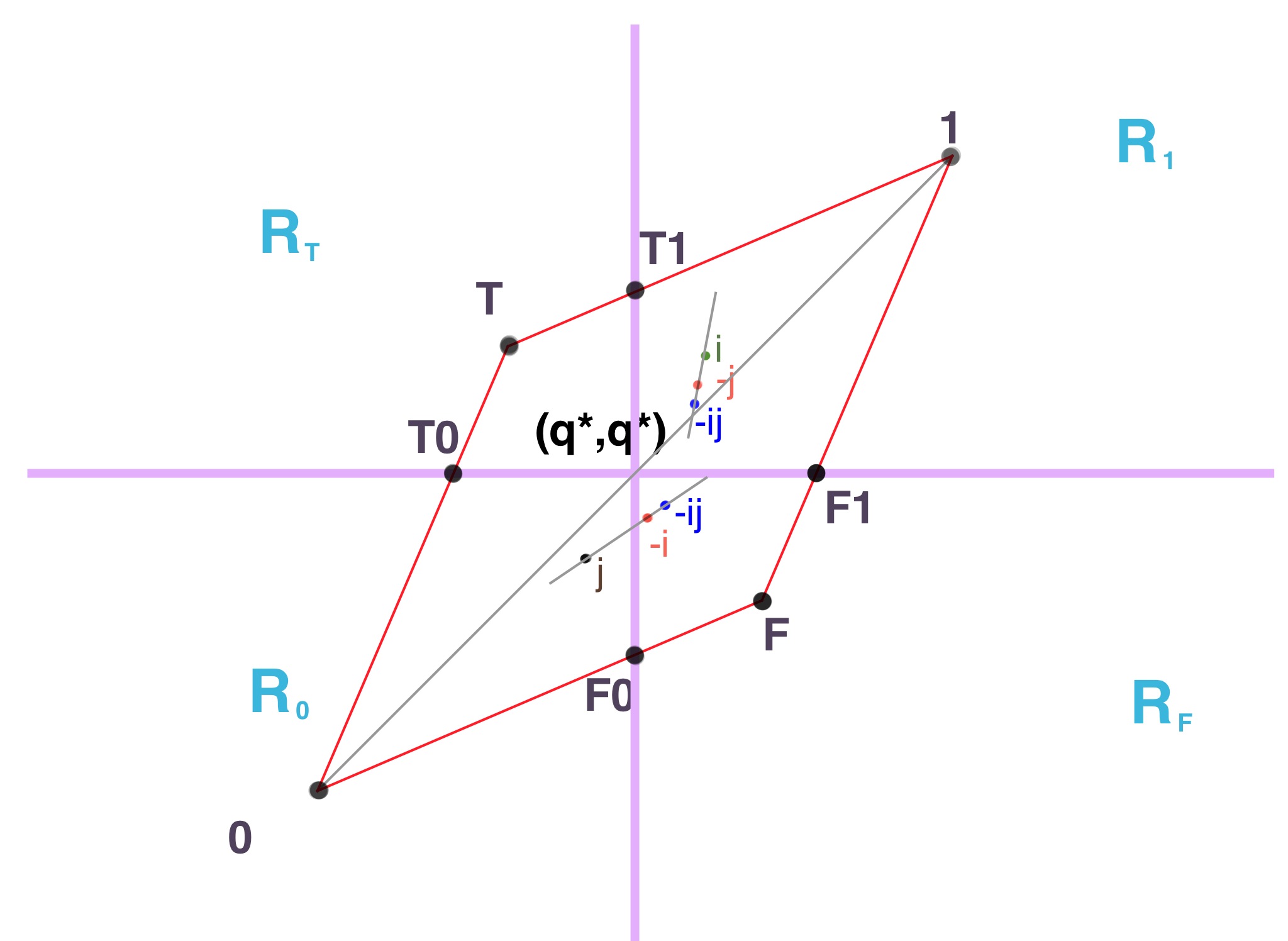
Now we will introduce the best response plot in detail. The best response plot is a plot which, given (the “average” strategy of the agents in ), maps it to the point . For example, would map to , and would map to . Because we assume , this map is a bijection. Since it is a bijection, we will abuse notation a little by using to represent .
The four pure strategies , , 0, 1 are mapped to four distinct points in the best response plot. We abuse notation and call these four points in the best response plot , , 0, 1.
We define to be the convex hull defined by the points in (recall is the set of pure strategies).
Recall that is the set of all possible best responses. We define the support of an agent’s strategy to be the set of all responses that the agent uses with non-zero probability. For example, for the strategy that is always reporting 1 with probability and ignoring the private signal received, its support is . For pure strategy like , its support is itself .
For , let
For example, when , is the upper left region. When , is the left part of axis (which actually is the intersection of and ).
Actually, we abuse notation in two further ways. First, given we define
to divide into four quadrants: . We also extend these quadrants to partition the entire plane.
Given a finite set of points , we define as the convex hull of . Given a convex set , let denote the interior points of and let denote the boundary of (so that is the disjoint union of and ).
We name some additional points of our best response plot. We define , , , , if they exist. (See Figure 2.)
Notice that in the best response plot, , , and , but may not be in . (See Figure 3.) When , if , then ; if , then . When , if , then ; if , then . It turns out that these two cases (i.e., whether lies in or not) create large differences in the structure of the equilibria.
Claim 4.2.
is an equilibrium iff ,
Proof.
is an equilibrium iff , any strategy in is a best response for player ; this means that . ∎
Note that we mentioned before that there is a bijection between and , for convenience, we sometimes write this claim as
4.2 Proof of Theorem 4.1
We will use the best response plot as a tool to compute all the equilibria of the peer prediction mechanism. The proof proceeds in three steps. First, we use the best response plot to find some symmetric equilibria. Second, we show that no asymmetric equilibria nor additional symmetric equilibria exist. At this point, we have classified all equilibria in terms of . The third step inverts the mapping from to to solve for the equilibria in terms of .
Symmetric equilibria
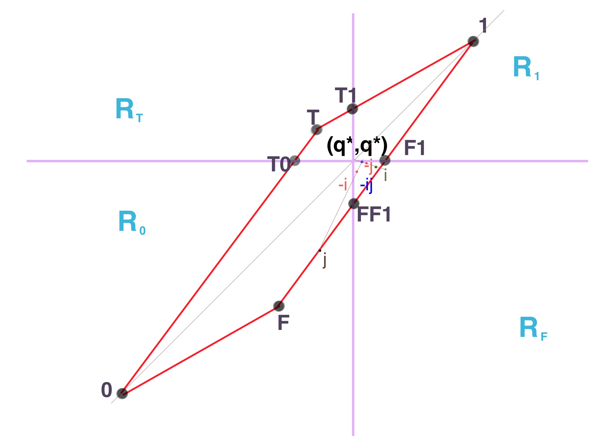
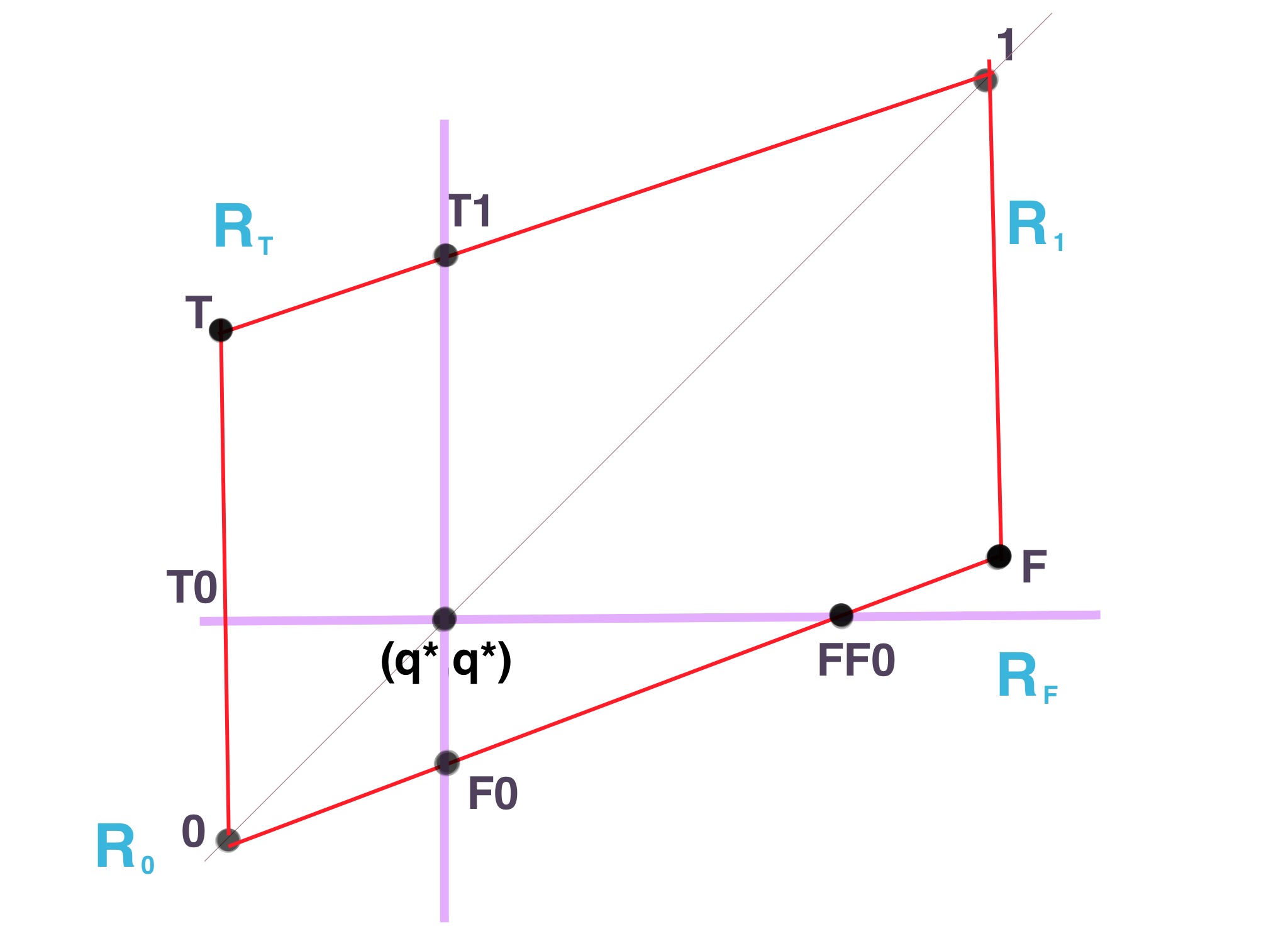
There are two basic cases: first and second . If is a symmetric equilibrium, recall, we will use to refer to it.
Lemma 4.3.
For each condition below, we prove existence of a set of symmetric equilibria of the peer prediction mechanism.
Proof.
Notice that it is always true that . There are two cases: or .
We first consider . is a symmetric equilibrium since if , (), then we have , and . Based on Claim 4.2, is a symmetric equilibrium. Similarly, are symmetric equilibria as well. is a symmetric equilibrium since if , (), then we have , and . Based on Claim 4.2, is a symmetric equilibrium. Similarly, are symmetric equilibria as well. is a symmetric equilibrium since if , , then we have , and . Based on Claim 4.2, is a symmetric equilirium.
Next, we consider ; the results are proved similarly. But notice that in this case, is not a equilibrium since . Also note, does not exist when , and does not exist when . ∎
There are no asymmetric equilibria
We will be aided by the following proposition, which states that once we have shown that all the are in the same quadrant, if even one agent is in the interior, then all must be .
Proposition 4.4.
For any equilibrium, if there exists such that for all , , and there exists an agent such that , then it must be that for all , .
Proof.
Because , we know that , meaning has full support. Based on Claim 4.2, we have . Then the average of for , is an extreme point of , which is a convex set. Since all are in , we will have . Now we examine agent , because , by the same reason we know as well. ∎
We now show that the peer prediction mechanism does not have asymmetric equilibria.
Lemma 4.5.
Let be a symmetric and positively correlated prior on , and let be a corresponding peer-prediction mechanism. There are no asymmetric equilibria of the mechanism.
Proof.
To prove Lemma 4.5 we will consider two cases: first and second . For each case we will prove the Lemma in two different steps. In the first step we will show that for any equilibrium, is in the same quadrant of the best response plot for all agents. In the next step we will show that, in fact, all the must be the same for all agents, and moreover must be one of the equilibria detailed in the statement of Lemma 4.3.
Case 1, Step 1: Showing that if , then all are in the same quadrant.
First, we show that either or . Second, we show that either or . This will complete step 1.
For the sake of contradiction, we assume that it is not the case that either or . Then there exist agent and agent such that and , which implies that and . If , then , which means . But this is a contradiction, due to Claim 4.2. The analysis for is similar.
The proof for either pr is similar to the previous proof when .
Case 1, Step 2: Showing that if , then all are the same and are equal to one of .
We prove the Claim when . The remaining cases proceed similarly.
We first consider when such that . By Proposition 4.4, we have .
Next we consider when . If then this a symmetric equilibrium . Otherwise, there exists such that either or . If , then based on Claim 4.2, , which means . Then the average of is an extreme point of a convex set . Since all are in , we will have . Now we examine agent , because , by the same reason we know as well. The proof for is similar.
The results for other quadrants are shown similarly. In summary, we show is an equilibrium iff all are the same and are equal to one of .
Case 2, Step 1: Showing that if , then all are in the same quadrant.
Notice that under the case , when , ; when , . We show the proof for and . The other case, when and , is analogous.
First, we show that either or . For the sake of contradiction, we assume that it is not the case that either or . Then there exist agent and agent such that and . If , then which means , but this is a contradiction based on Claim 4.2. The analysis for is similar.
But to show either or we cannot use the same approach as before. We will show it under two cases by contradiction:
First, we consider when . (This is illustrated in Figure 3 when all points are in upper half-plane):
If , and , combining with , we obtain , . Then while which is a contradiction. If , then while , which is a contradiction.
Next we consider when . (This is illustrated in Figure 3 when all points are in lower half-plane):
If , and , we have , . Then while , which is a contradiction.
If , and , then . But even if , we do not have the fact that , since and can be , whose support set only contains . We cannot obtain a contradition using the previous way. We prove it in two steps: first, we show that is strictly less than ; second, we show that when is strictly less than , cannot be strictly greater than .
Case 2, Step 2: Showing that if , the all are the same and are equal to one of if or if .
The analyses for all points in and are similar to the previous analysis under the case where . We will show the analyses for and here.
First, if all points are in the same quadrant and there is such that is not on the boundary, then , based on Proposition 4.4. So then we only need to consider the case when all points are on the boundary.
If , then such that . We have . Then since is an extreme point and all points are in , we have and based on the same reasoning, , as well.
If , when , then this is a symmetric equilibrium. Otherwise:
- (a)
When such that :
In Claim 4.2, which means . Then since is an extreme point of and , we have . We also have based on the same reason since . So we have .
- (b)
When such that :
Based on Claim 4.2, which means situation (b) is impossible, that is, there does not exist any such that .
- (c)
When such that or :
Based on Claim 4.2, . is a point and let denote it. . Then since is an extreme point, we have . So is while when or . However, we already proved there does not exist any such that , so situation (c) cannot happen as well. ∎
In summary, we show is an equilibrium iff all are the same and are equal to one of .
Now we consider the case when . Then , and, based on a similar analysis as before, we show that is an equilibrium iff all are the same and are equal to one of .
Translating from best response plot back to strategy profiles
We calculate the strategies that are mapped to .
For , setting and in Equation 2 we get
For , setting and in Equation 2 we get
For , this is analogous to the case where players receiving 0 always tell the truth and players receiving 1 sometimes lie, and the result follows by the above calculations by simply switching the labels 0 and 1. Before we showed that . Switching the labels gives us:
For , this is analogous to the case where players receiving 0 always lie and players receiving 1 sometimes lie, and the result follows by the above calculations by simply switching the labels 0 and 1.
5 Making truth-telling focal among the informative equilibria
In this section, we first introduce a useful concept, line sets, and then we build up a sequence of lemmas that will be useful in Section 6. Along the way, we show Theorem 5.4, that there exists a proper scoring rule that makes truth-telling have higher payoff than any other informative equilibrium.
5.1 Line Sets
We now introduce notation that highlights the role of three constants that will emerge as the key defining parameters of any proper scoring rule. Useful related observations related to scoring rules appear in Appendix A.
Definition 5.1.
We define a line-set as a set of linear functions where , . We say a proper scoring rule and a line-set correspond if
Notice that there is a natural mapping from a line-set to payoff fucntion matrix .
It is useful to note that arbitrary convex functions can be converted into scoring rules as follows.
Fact 5.2.
[9] Given any (strictly) convex, differentiable function , and any arbitrary function , the function is a (strictly) proper scoring rule. Note that the first three terms are the negation of the Bregman divergence of .22 2 A more general version in higher dimensions also holds, as does a converse of the equivalence. However, we do not use these stronger statements here.
As a consequence, for a certain class of , , , and , one can find a corresponding proper scoring rule.
Lemma 5.3.
Given any line-set (or payoff function) with and , there exists a strictly proper scoring rule that corresponds to this line-set.
Proof.
Essentially, appealing to Fact 5.2, our goal is to produce a strictly convex function and an arbitrary such that the proper scoring rule constructed via the Bregman divergence matches the desired scoring rule at and . This gives constraints on that and , and .
These two tangent lines to , at and , intersect at . Recall that . Thus, between and , one can construct as a quadratic Bezier curve given and their intersection at . Outside of , one can extend with a spline. ∎
5.2 Making truth-telling focal among informative equilibria
Informally, the following theorem states that under a weak condition, there is a line-set such that the proper scoring rule satisfying this line-set makes truth-telling focal among all informative equilibria.
Theorem 5.4.
Let be a symmetric and positively correlated prior over binary signals. Then there exists such that for any strictly proper scoring rule that corresponds to a line-set with , the payoff of is no less than that of any other informative equilibrium. Moreover, if , , and , the payoff of is strictly greater than that of any other informative equilibrium.
Motivation for Best Response Payoff Plot
We want to select a proper scoring rule in order that truth-telling will have higher expected payoff than any other equilibrium. If we just compute the average payoffs of agents playing symmetric strategies, then even for the simplest proper-scoring rules, these payoff curves are paraboloid, and hence difficult to analyze directly. Instead we will analyse the payoffs of the best-responses. Because the best responses are the same in each quadrant, the best response payoff plot is piece-wise linear for all proper scoring rules, which makes the analysis tractable.
A key tool will be the best response payoff plot which is defined by extending the definition of the best response plot to include not only the best response strategy, but additionally the expected payoff of playing this best-response strategy. A contour on the plot corresponds to a set of points that have identical best response payoffs. A key observation is that for any equilibrium, agent ’s payoff is equal to his best response payoff (this is not true for non-equilibrium strategy profile).
Since the best response payoff of any equilibrium is equal to that equilibrium’s payoff, the contour plot can be used to compare the payoffs of different equilibria.
The rest of this section will formally define the best response payoff and the contour plot, and finally give a proof outline. The actual proof is in Section 5.3.
Best Response Payoff
We extend the definition of the best response plot of Section 4.1. We only consider symmetric strategies (because we have shown that all the equilibria are symmetric). However, we fix some player and consider his best response when all of the other players are playing some symmetric strategy ; we write the payoff of this best response as .
Now notice that we can express , the probability a priori that a player receives a signal of one, in terms of and :
This allows us to express the best expected payoff only in terms of and .
Contour Plot
We introduce the notion of a contour plot depicting , where the and axes are, respectively, and . A contour on a contour plot corresponds to the set of points such that
for some constant . An important observation is that for any equilibrium, agent ’s payoff is equal to his best response payoff (this is not true in general).
Proof Outline
The main tool we use to prove Lemma 5.4 is the contour plot. Since the best response payoff of any equilibrium is equal to that equilibrium’s payoff, the contour plot can be used to compare the payoffs of different equilibria. The plot is centered at and thus the four quadrants, , correspond to whether each of and is greater or less than . By the definition of , each quadrant corresponds to a different best response.
We will first show that in each quadrant, a contour is actually a line whose slope depends only on the ratio of the slopes, , from a -line set. These lines make it easier for us to compare the payoffs of various equilibria: the further a line is from the center of the plot, the higher its payoff is. We want to be able to compare the lines that go through the equilibrium points in some way, but unfortunately, the equilibria are not necessarily all in the same quadrant. Surprisingly, we are able to define a mapping that translates lines from one quadrant to another in a way that preserves the payoffs at equilibrium and does not depend on the values of and . When all translated equilibria are in the same quadrant, we will show that truth telling is an extreme point of the convex hull of all translated informative equilibria. We do so using Lemma 5.10, which pairs up equilibria such that the lines going through each pair of equilibria are parallel, and such that the truthful equilibrium is on the highest payoff line amongst the informative equilibria (see Figure 4). Once we show Lemma 5.10, we can see by taking and such that the slope of the contours in equals the slope the line incident on the two extreme equilibria adjacent to truth-telling, we ensure that the truthful equilibrium pays at least well any other equilibrium (see Corollary 5.11). Based on Lemma 5.10 and Corollary 5.11, we show Lemma 5.4.
5.3 Proof of Theorem 5.4
Our goal is to find a -line set, making the truthful equilibrium at least as good as any other equilibrium. Since the difference between the payoffs of any two equilibria does not depend on , we can assume now without loss of generality, but will in Section 6 discuss the value of in the context of maximizing the payoff of truth-telling with respect to other equilibria. (We will see that the result of Theorem 6.4 is obtained by properly choosing .)
The claim below will help us construct a mapping that translates lines from one quadrant to another in a way that preserves the payoffs at equilibrium and does not depend on the values of and .
Claim 5.5.
- 1.
In every quadrant, the contour of the best response payoff function is a line.
- 2.
The slope of the contours of the best response payoff function in both and is and does not depend on the parameters .
- 3.
The best payoff of any point can be decomposed as the sum of the best payoff of and the best payoff of
Proof of Claim 5.5.
Recall that we assume .
| Quadrant | Best response payoff when other players play (x,y) |
|---|---|
In Table 1, the best response for each quadrant is the best response of agent when is in that quadrant. This comes from the fact that
and that the best response of a player who gets bit is if , and if . Part (1) of the claim follows immediately from Table 1. We can also observe from Table 1 that when , the slope of the contours in both and are , so part (2) follows. Part (3) of the claim follows since in the best response plot, , and are in the same quadrant. If they are in the region, according to Table 1, the best response payoff of is
which is a sum of the best payoff of and . The proof is similar in other quadrants. ∎
Definition 5.6.
is a translation map if for any point , the mapping is in and if and have the same payoff.
Now we will construct a map and prove that is a translation map.
Definition 5.7.
Define as follows. For in , . For in , let be the intersection point of the contour line and . For in , let be the intersection point of the contour line and . For in , where means the -coordinate of , and means the -coordinate of .
Claim 5.8.
is a translation map.
Proof.
It is clear that is in ; now we need to prove that it preserves the best expected payoff. Based on Claim 5.5, we know the slopes of the contours in both and do not depend on and , so does not depend on and . According to the definition of a contour, preserves the best expected payoff of points in and . For points in , since we know the best payoff of can be decomposed as the sum of the best payoff of and based on Claim 5.5 and preserves the best expected payoff of and (because they are in or ), we can see also preserves the best expected payoff of points in . ∎
We will show the analysis for . the case when is analogous.
Recall that in Section 4, we defined as an equilibrium in which agents play truthfully when they receive bit , and randomize when they receive bit . This equilibrium is the convex combination of and that has , and is therefore at the boundary of quadrants and . We also defined , and in a similar fashion.
Having constructed the translation map, we can translate all equilibria to the same quadrant , to ease comparisons among them. If we wish for truth-telling to be focal, we need to tune the slope of the contours in , which will turn out to be a linear programming problem.
Definition 5.9.
Notice that in the region, the best response payoff is
so the slope of the contours in is
We denote this slope by .
Before we tune the slope , we will first show, in the next lemma, that truth telling is an extreme point of the convex hull of all translated informative equilibria.
Lemma 5.10.
Given positively correlated common prior Q, given , consider the convex hull of a set of points which are derived using the translation map to translate all informative equilibria to the region.
- Case 1 (when
-
In this case, we have three different cases based on the number of equilibria.
- If :
-
is an extreme point, and share the same facet, and and share the same facet;
- If :
-
is on the line segment whose endpoints are and , so is not an extreme point of
- If :
-
is an extreme point, and share the same facet, and and share the same facet;
- Case 2. (when )
-
, and and share the same facet.
We prove Lemma 5.10 below, but first, we discuss its consequences. Given Lemma 5.10, we will tune the slope of contours in to make truth-telling focal. According to Lemma 5.10, if this slope is strictly between the lines which are incident on truth-telling and its adjacent extreme equilibrium, we can ensure that the truthful equilibrium pays at least well any other informative equilibrium. When , this is not possible since is not an extreme point in this case; however, one can avoid this case by picking .
The above results are stated in detail in the below corollary.
Corollary 5.11.
Given positively correlated Q, we show how to make truth-telling focal among the informative equilibria. We state results for the case when ; the case when is analogous.
- Case 1 :
-
Truth-telling can be focal among the informative equilibria and will be so if and either of these two restrictions on holds:
- (1)
-
,
- (2)
-
,
- Case 2 :
-
There is no way to make truth-telling focal among the informative equilibria, since . However, truth-telling can have (non-strictly) greatest payoff among them if , ,
Proof of Theorem 5.4.
Based on Corollary 5.11, given positively correlated prior , we can select and to make truth-telling focal if . ∎
Proof of Lemma 5.10.

Given positively correlated Q and , we discuss the problem under the following possible cases:
Case 1: when there exist eight or nine equilibria ()
There are nine equilibria iff the pure strategies are in different quadrants. Since we have , there are nine equilibria iff .
Table 2 contains the coordinates of all nine equilibria.
| Equilibrium | ||
|---|---|---|
The four claims below show that truth-telling is an extreme point of the convex hull of all translated informative equilibria.
Claim 5.12.
When , the lines that are incident to the following four pairs of points are all parallel to each other. Moreover the slope of those parallels is always greater than 0.
Proof.
The claim follows immediately from computing the slope of each line, which are all equal to
This slope is always greater than 0. ∎
Claim 5.13.
When , going from toward , the order of the four parallels is as follows: .
Proof.
To prove the claim, we compute the values of the intersection points of the following four pairs
with the -axis and compare them.
The -coordinates of the intersection points are given by:
Then we compare them:
according to the fact that
We see that
according to the fact that
Finally,
Claim 5.14.
When , , if and if ,
Proof.
follows immediately from the x-coordinates of and . Since the slope of the line incident to and is always greater than 0, . ∎
Claim 5.15.
If and , then
Proof.
For Claim 5.15, if , , then , , and will lie in one line since
Then the payoff is highest among all informative equilibria iff the slope of the contour line is
which is the slope of the parallels in Claim 5.12, or one of and will be greater than the payoff of . But the payoff of must be equal to the payoff of , which means the payoff of cannot be strictly greater than any other informative equilibria. ∎
Given the above claims, is an extreme point of the convex polygon of all translated informative equilibria. and are ’s two adjacent extreme points. We also know that the best response payoff is a linear function with parameters in region , according to Table 1. If we think of the best response payoff as an objective function in a linear program and of all translated informative equilibria as feasible points, we can see it is possible to properly choose such that the best response payoff of is the global optimum among the best response payoffs of all informative equilibria, since is an extreme point. To make the best response payoff of exceed the best response payoff of , we can see that must be greater than 0.
- 1.
If , the payoff of will always be the same as the payoff of since when . If the slope of the contour line is
then the payoff of () is greater than the payoffs of other informative equilibria since the contour line incident to will be further from than contours incident to other informative equilibria.
- 2.
If , if we set such that the payoff of is equal to the payoff of , then the slope of the contour will be strictly greater than the slope of the line incident to and and strictly less than the slope of the line incident to and . The payoff of will be strictly greater than the payoffs of other informative equilibria since is an extreme point and the contour line incident to is not incident to other points, based on Claim 5.13.
This completes Case 1.

Case 2: There exist seven equilibria
There are fewer than eight equilibria iff pure strategies are not in different quadrants. must be in since . and must be in and respectively. So there are less than eight equilibria iff is in and not in , which happens when . In this case, neither nor is an equilibrium,
and
Now we can see is an extreme point of all translated informative equilibria and and are ’s two adjacent extreme equilibria. If we set the payoff of equal to the payoff of , then the slope of the contour will be strictly greater than the slope of the line incident to and and strictly less than the slope of the line incident to and . The payoff of will be strictly greater than the payoffs of other informative equilibria since is an extreme point and the contour line incident to is not incident to other points, since . ∎
6 Optimizing the Gap
In this section, we continue to focus only on the informative equilibria. We seek to design a payoff function, derived from a proper scoring rule, that maximizes the advantage (gap) of the payoff of the truth-telling equilibria over the payoffs of any other informative equilibrium.
Even though we classify all equilibria in Theorem 4.1, it is still challenging to obtain the optimization result in Theorem 3.5. Firstly, we must determine what kind of proper scoring rules make truth-telling have an advantage over all informative equilibria. Secondly, we must determine, when truth-telling is better than other informative equilibria, which informative equilibrium is the second best equilibrium. Thirdly, we must determine which proper scoring rule maximizes the advantage truth-telling has over the informative equilibrium which have the second largest expected payoff, over all Peer-prediction mechanisms with payoffs in .
Without the help of our best response payoff plots, the above steps are extremely complicated even in binary setting. However, with the help of our best response payoff plots, the above steps become approachable. We will show an important observation first: we can tune proper scoring rules by tuning the break-even point and the slope of contours. We divide our proof into two steps:
- 1.
Fix the break-even point and tune the slope of contours in region to such that the advantage of truth-telling is optimized, over all Peer-prediction mechanisms with payoffs in .
- 2.
With , tune such that the advantage of truth-telling is optimized globally.
6.1 Attainable Priors
In this section, we introduce the concept of an attainable prior, and use it to divide the space of possible priors into three regions. For the first two regions, we show that we can obtain mechanisms with optimal gap and for the third region, we show that there is no mechanism that has optimal gap but we can obtain mechanisms with gap arbitrarily close to the optimal value, which appears as Theorem 6.4.
Recall that (see Definition 2.5) is the payoff matrix of a line-set (which corresponds to a proper scoring rule). Now we consider a set of payoff functions where the maximal payoff is and the minimal payoff is .
Definition 6.1.
Define to be the set of payoff functions with payoffs between and . That is, let For positively correlated Q, let be the set of equilibria under payoff function . Let
be the gap between truth-telling’s payoff and the maximal payoff of all other informative equilibria.
For any given symmetric and positively correlated , we would like to
- 1.
Solve
- 2.
Either find such that or; if such doesn’t exist, then , find such that .
Definition 6.2 (Attainable Prior).
We call a prior attainable if such that ; otherwise, we call the prior unattainable.
We divide the positively correlated priors into three regions which correspond to three payoff functions which (almost) attain the optimal gap . These three regions are shown in Figure 6.

Definition 6.3.
where
,
,
, and
,
where ,
.
Note that and contain attainable priors, while contain unattainable priors.
6.2 Optimization Theorem: Statement and Proof Structure
Theorem 6.4.
For any binary, symmetric, positively correlated, and signal asymmetric prior , with (the case is analogous),
- 1
-
If , then
- 2
-
If , then
- 3
-
If , then
where
, , and
, ,
, and
.
We note that the actual form of the optimal payoff functions is quite simple, especially in and , where they only have one parameter to tune.
Definition 6.5.
We define as a normalization function and
Recall from Definition 6.1 that is the payoff functions with payments between 0 and 1.
Lemma 6.6.
Proof.
For all , ; so . For all , we have , so . Then the result follows. ∎
This allows us to translate a constrained optimization problem into an unconstrained optimization problem.
Definition 6.7.
We define as a function mapping to a payoff function such that and and .
Remark 6.8.
If then is a proper scoring function, and, restricted to this case, is surjective onto all .
Remark 6.9.
Notice that by Definition 5.9, in the region, the slope of the contours is
so can be represented as .
Proof Overview for Theorem 6.4
We will show three lemmas to prove Theorem 6.4. In the first lemma (Lemma 6.11), we show that the gap we want to optimize depends only on the value of and the slope of contours in the region. Let
The goal then is to solve ; notice that
Recall that by Theorem 4.1, for a fixed prior, the set of equilibria are determined by . Additionally, by Definition 5.9, the contours of the best response plot are determined by . So Lemma 6.11 formally states that the contours of the best response payoff plot encode all the information that is relevant to optimizing the payoff gap.
In the second lemma (Lemma 6.14), to show how to optimize when is fixed, we define so that for any ,
In the proof there are two main cases.
In the first case, : This corresponds to the case of 7 equilibrium. Here, by Lemma 5.10 and Corollary 5.11, the points in the best response plot that limit the range of are and . For the same reason, for any that makes focal the equilibrium with payoff closest to that of must be either or . It will turn out that the gap is maximized by making the payoffs of and equal.
In the second case, : This corresponds to a setting where there are 8 or 9 equilibrium. This is similar to the first case except that now and are the constraining equilibria. It will turn out that the gap is maximized by making the payoffs of and equal. (In the first case, was not an equilibrium, but in this case it is).
In the third lemma (Lemma 6.15), we will solve
Once we know how to optimize for any fixed , the third lemma shows how to optimize . To prove Lemma 6.15, we map out the payment for different while making sure that
- 1.
the payoffs of and are equal; or
- 2.
the payoffs of and are equal.
In Case 1, as moves from to , the gap first increases then decreases. Similarly, in Case 2 as moves from to , the gap first increases then decreases.
At this point there are two settings. In the first setting, the gap in Case 1 is maximized when . In some sense, this is the “good” setting because if there are 7 equilibria, and so Case 1 gives the correct analysis. Here we should take the maximum of Case 1 and Case 2.
In the second setting, the gap in Case 1 is maximized when we have that . Here we cannot use the maximum from Case 1 because when there are more than 7 equilibria (in particular, we must worry about the payoff of ). But the analysis of Case 1 assumes that there are only 7 equilibria (and, in particular, that is not an equilibrium). In this setting, the best permissable Case 1 solution does not exist. Recall that to have 7 equilibria and obtain the gap in Case 1, we need , but because the gap for different are first increasing then decreasing, the gap will increase as we approach the boundary from the right side.
In this setting we should choose between the value of Case 1 at or the maximal value of Case 2 , whichever is greater. If the maximal value is the maximal value of Case 2, then we can obtain a mechanism that has this opitmal gap, and this mechanism has 9 equilibria. If the maximal value is at , then we cannot obtain a mechanism with optimal gap since we need to have 7 equilibria. But we can obtain a gap that arbitrarily approaches the maximal value if we set arbitrarily close to .
Finally, when we plug in the optimal and , we get the payment schemes as stated in the theorem. The regions correspond to the different cases/settings above. In we use the Case 1 maximum; in , we use the Case 2 maximum, and in we use the Case 1 analysis, as limits to from the right.
This will prove Theorem 6.4.
We now formally state the three lemmas. We will defer their proofs, and instead first show how they combine to prove Theorem 6.4.
Lemma 6.10.
If , only depends on and on . Thus
is well defined.
Corollary 6.11.
For any , ,
only depends on and on , which is the slope of the contours in . Thus
is well defined.
Remark 6.12.
Definition 6.13.
Lemma 6.14.
Lemma 6.15.
- 1.
There exist , such that
and , .
- 2.
If then is either attained at either or . If then is either attained at either or the right limit of .
- 3.
and when , ,
We defer the proofs of these lemmas, and first show how Theorem 6.4 follows from them.
Proof of Theorem 6.4.
We will consider three cases:
- Case 1 (when )
-
When , if the mechanism has truth-telling as a strict Nash equilibrium, it must have seven equilibria. In this situation, is always . So is attained at . We also know by Lemma 6.15 that . Additionally, we are in (by the definition of ).
- Case 2 (when )
- Case 3 (when )
∎
6.3 Proof for Lemma 6.10 and Corollary 6.11
Proof of Lemma 6.10.
Let be . Then this payoff function only depends on . However, we have
| (10) | ||||
It follows that only depends on and . However,
The last equality follows from the fact that we merely shifted and scaled all inputs. Since only depends on , the Lemma follows.
∎
6.4 Proof for Lemma 6.14
Proof of Lemma 6.14.
We show this Lemma in two cases. In each case, we will optimize the gap between the best equilibrium and the second best equilibrium; there are two possible second best equilibria. We will prove that once we set the parameters such that the payoffs of these two possible second best equilibria are same, the gap is optimized.
(1) If :
Based on Lemma 5.10 and Corollary 5.11, there will be seven equilibria,
and
So
Since is given, let
We have
We will show both is increasing and is decreasing whenever .
This is the important range of ’s because being focal implies that
The translation map is defined in Table 2.
It follows that obtains its maximum when , which means
So the payoff contour lines will go through point and point , which implies that the slope of the contour lines is
It is now left to show is increasing and is decreasing.
To show that is increasing, we show
| (11) |
From this we can see is increasing since for any two increasing functions , is still a increasing function.
| (12) |
To arrive at Equation 11 we must compute .
It will help to better understand . By Lemma 6.10 we know that there exist functions and such that:
So and
From Table 1, we know the best payoff of point in the quadrant is
The payoff function is , so . To calculate the payoff of , we replace with and with since is the point in that represents . Similarly, we calculate the payoff of . Now we have
| (15) | ||||
We would like to compute more explicitly. Fix an arbitrary , and let Then we know that
| (16) |
Claim 6.16.
When has seven equilibria,
Proof.
Since
| (17) |
we can see
∎
The first inequality follows from the bound on in (17). So
| (18) | ||||
The first equality is from Equation (16). The second equality is from Claim 6.16 and the fact that is minimized at either or . The third line follows from equation (10).
Finishing up we have that:
| (19) | ||||
The second line is from (15). After we plug value from (18) and translation map value from Table 2, we obtain the third line. The fourth line is manipulation.
This verifies Equation 11.
Similarly, we replace with
We can see is decreasing since when k is increasing, is decreasing and is increasing.
(2) If :
Based on Lemma 5.10, there will be nine or eight equilibria, and
if is focal. In the previous case, the second best equilibrium is or while in this case, the second best equilibrium is or . Now we will use the same method in the previous case to prove that once we set the payoff of equal to the payoff of , the gap between the best equilibrium and the second best equilibrium will be optimized.
The gap we will optimize is the minimum of and , where
To calculate them, we need to give an explicit form of . Similarly, we have the following claim:
Claim 6.17.
When has nine equilibria,
Proof.
Since ,
To prove is increasing and is decreasing, we will write them explicitly. We omit the proof here since the calculations are similar to the previous case, replacing with .
Once we have proved is increasing and is decreasing, the gap will be optimized when
6.5 Proof for Lemma 6.15


Proof of Lemma 6.15.
The framework of the proof is as follows:
- 1.
Show that for some , to be defined later.
- 2.
Show that
- 3.
Show that for from above, there exists a point such that for is increasing, and for is decreasing. Similarly for and
- 4.
Show that 2) and 3) imply that there exists a between (or equal to) and such that .
- 5.
Show that
- 6.
Show that by calculating the coordinates of and proving that .
Part (1) Show that for some , to be defined later:
We show part (1) in two cases:
:
Let
Based on Lemma 6.14,
The first line follows from (19). After we plug in it, we obtain the second line.
Then we show
:
Let
Based on Lemma 6.14, . Like we did when , after all substitutions, we will get
Part (2) Show that :
We will show Part (2) in two cases:
Now we will show
when .
We first show
Once we show it, it’s clear that since is a bijection between and itself.
By arithmetic manipulation, we get:
Similarly, we show
then it is clear that
when since is a bijection function between and itself.
Part (3) Show that for from above, there exists a point such that for is increasing, and for is decreasing. Similarly for and :
We will show that is first increasing and then decreasing.
For , we will use two facts to prove it:
- 1.
- 2.
The derivative is a rational function where the denominator is positive and the numerator is a degree 2 polynomial.
The first fact implies that the derivative changes sign ( or ) odd times. The second fact implies that the derivative changes sign at most two times. So they implies that the derivative changes sign only once at a critical point. We define this critical point as . Then the result follows.
Now it is left to show the two facts. By simple observation, We have is positive when and . Then the first fact follows. By taking derivatives, the second fact follows.
Since is a increasing function, is also first increasing and then decreasing when .
Similarly, when , we can also prove that both and are first increasing and then decreasing when .
Part (4) Show that 2) and 3) imply that there exists a between (or equal to) and such that :
We begin by proving that there exists a point between and such that .
If , then and the results follow, so we assume . Then we will show
| (20) |
Once we show it, by the intermediate value theorem, we know there exists between and such that .
To show (20), we use the result in Part (2): .
Part (5) Show that :
Now we prove that maximizes . Without loss of generality, we assume . We prove it by contradiction:
We assume there exists such that both and are greater than . Then we show the contradiction in two cases:
Case 1:
We have . So is decreasing at , which is a contradiction.
Case 2:
We have . So is increasing at , which is a contradiction.
Part (6) Show that :
We first show to help calculate the mechanisms:
| (21) |
So the payoff function will be or , where will be calculated later.
Now we will use this property to obtain :
Show :
Now we will calculate the coordinates of .
We solve the equation to get a root between and . We know that . We also have two additional nontrivial roots
But is greater than since
So
Let . After substitutions, we have
When , by Claim 6.16, we have is the maximum which is . We also have . Since depends on the four values of , given the three values and the coordinates of , we can solve
So
where
Show :
We solve the equation . Besides , we also have two additional nontrivial roots
Notice that
so . After substitutions, we have
By a similar method to that used to obtain , we get
where
Show :
To calculate , we first prove that is the minimum . Then combining with the fact that is the maximum according to Claim 6.16, we only have two values left to calculate. We solve the rest of the values by values and otain
where
,
Now we begin to show that is the minimum :
We first show that when . Once we show it, by a similar method to that used to prove (21), we will get the result. It is now left to show :
Since there is only one intersection point of and , so when , one of and must be less than another. Notice that we have
and
So when is close to since is decreasing now. Combining with the fact that when , one of and must be less than another, we have when .
∎
7 Punishing all- and all- equilibria to complete the proof of the main theorem
Finally, we would like to suitably punish the non-informative equilibria, so that, combining this with the mechanisms of Theorem 6.4, truth-telling is focal with respect to all equilibria. By the following claim, if such a penalty only depends on other players’ reports, then it does not affect the set of equilibria. We therefore punish an agent if all the other agents report the same signal.
Claim 7.1.
Adding an arbitrary function of the other players’ reports to the player payments does not change the set of equilibria.
Proof.
Adding a term to agent ’s payoff that is only based on the actions of the other agents does not alter the set of equilibrium because the marginal gains/losses from unilateral deviation remain unchanged. ∎
There is a possible issue with this approach: it might be the case that all players receive the same signal and that the truthful equilibrium will be penalized. Under certain conditions, this penalty will affect any informative equilibrium with low probability. Thus the punishment’s expected impact on informative equilibria will be overcome by the advantage of the truth-telling equilibrium’s payments that we constructed in Theorem 6.4. On the other hand, the and equilibria will fully bear this punishment, and hence have lower payoff than truth-telling.
Theorem 3.5.
(Main Theorem (Restated)) Let be a binary, symmetric, positively correlated and signal asymmetric prior, and let be the maximum probability that a fixed set of agents receive the same signal (either all or all ). Then
- 1.
when the prior is attainable; when the prior is unattainable.
- 2.
Let when the prior is attainable; let when the prior is unattainable. If , our (or when is unattainable) makes truth-telling focal.
Note that once truth telling is focal, we can renormalise so that payments are between 0 and 1. We also note that only depends on and .
Proof.
Part (1) has already been proved in Theorem 6.4.
We start to prove part (2) now:
Recall that we design the mechanism (or )identical to (or ) except that we will issue a punishment of to an agent if all the other agents play all or all .
By our assumption on , we know that . Because is the average of these two values, we have .
By Claim 7.1 the equilibrium of (or ) are the same as those of (or ).
On the one hand, the expected payment of truth-telling has decreased by at most because in the truth-telling equilibrium, all agents report their true signals, and for any set of agents, all these signals are identical with probability at most . However, . If is unattainable let . Then the payment for truth-telling in (or is still greater than the payment for any other non-informative equilibrium (note that the payments for all equilibria only decreased).
On the other hand, the payment for the all zero or one equilibrium is now at most . And so truth-telling now pays more than the all 0 or all 1 equilibria. ∎
8 Future Directions
Extending our mechanism to a more general setting (e.g. non-binary setting, asymmetric priors, and mechanisms where the prior is not known) are interesting and challenging directions for further work. We briefly discuss the challenges in these directions. In the non-binary setting, the number of equilibria increases exponentially (this can likely be handled via extensions of the current techniques). However, the space of proper scoring rules also becomes more complicated. We hope that with the correct generalization of our main technical tool, the best response plots, our results can extend to this case as well. We are also hopeful that our results may extend to asymmetric priors (when the positive correlation requirement holds), but this requires additional technical work. We do not (yet) see inherent barriers to this extension. Certainly, removing the common prior assumption would make the mechanism more realistic. However, we note that if the prior were not known to the mechanism, then results as strong as ours would not be possible. This is because the agents can always permute their signals; if the prior were not known by the mechanism, such a strategy would always pay at least as well as truth-telling.
References
- [1] Crémer, J. and McLean, R. P. 1985. Optimal selling strategies under uncertainty for a discriminating monopolist when demands are interdependent. Econometrica 53, 2, 345–361.
- [2] Crémer, J. and McLean, R. P. 1988. Full extraction of the surplus in bayesian and dominant strategy auctions. Econometrica 56, 6, 1247–1257.
- [3] Dasgupta, A. and Ghosh, A. 2013. Crowdsourced judgement elicitation with endogenous proficiency. In Proceedings of the 22nd international conference on World Wide Web. International World Wide Web Conferences Steering Committee, 319–330.
- [4] d’Aspremont, C. and Gérard-Varet, L.-A. 1982. Bayesian incentive compatible beliefs. Journal of Mathematical Economics 10, 1, 83–103.
- [5] d’Aspremont, C. and Gérard-Varet, L.-A. 1979. Incentives and incomplete information. Journal of Public Economics 11, 1, 25–45.
- [6] Faltings, B., Jurca, R., Pu, P., and Tran, B. D. 2014. Incentives to counter bias in human computation. In Second AAAI Conference on Human Computation and Crowdsourcing.
- [7] Gao, X. A., Mao, A., Chen, Y., and Adams, R. P. 2014. Trick or treat: putting peer prediction to the test. In Proceedings of the fifteenth ACM conference on Economics and computation. ACM, 507–524.
- [8] Ghosh, A., Ligett, K., Roth, A., and Schoenebeck, G. 2014. Buying private data without verification. In Proceedings of the fifteenth ACM conference on Economics and computation. ACM, 931–948.
- [9] Gneiting, T. and Raftery, A. E. 2007. Strictly proper scoring rules, prediction, and estimation. Journal of the American Statistical Association 102, 477, 359–378.
- [10] Goel, S., Reeves, D. M., and Pennock, D. M. 2009. Collective revelation: A mechanism for self-verified, weighted, and truthful predictions. In Proceedings of the 10th ACM conference on Electronic commerce (EC 2009).
- [11] Jurca, R. and Faltings, B. Incentives for answering hypothetical questions. In Proceedings of the 1st Workshop on Social Computing and User Generated Content (SC 2011). ACM.
- [12] Jurca, R. and Faltings, B. 2006. Minimum payments that reward honest reputation feedback. In Proceedings of the 7th ACM conference on Electronic commerce (EC 2006).
- [13] Jurca, R. and Faltings, B. 2007. Collusion-resistant, incentive-compatible feedback payments. In Proceedings of the 8th ACM conference on Electronic commerce. ACM, 200–209.
- [14] Jurca, R. and Faltings, B. 2008. Incentives for expressing opinions in online polls. In Proceedings of the 9th ACM conference on Electronic commerce (EC 2008).
- [15] Jurca, R. and Faltings, B. 2009. Mechanisms for making crowds truthful. J. Artif. Int. Res. 34, 1.
- [16] Kamble, V., Shah, N., Marn, D., Parekh, A., and Ramachandran, K. 2015. Truth serums for massively crowdsourced evaluation tasks. arXiv preprint arXiv:1507.07045.
- [17] Lambert, N. and Shoham, Y. 2008. Truthful surveys. Proceedings of the 3rd International Workshop on Internet and Network Economics (WINE 2008).
- [18] Miller, N., Resnick, P., and Zeckhauser, R. 2005. Eliciting informative feedback: The peer-prediction method. Management Science, 1359–1373.
- [19] Prelec, D. 2004. A Bayesian Truth Serum for subjective data. Science 306, 5695, 462–466.
- [20] Radanovic, G. and Faltings, B. 2015. Incentive schemes for participatory sensing. In Proceedings of the 2015 International Conference on Autonomous Agents and Multiagent Systems. International Foundation for Autonomous Agents and Multiagent Systems, 1081–1089.
- [21] Riley, B. 2014. Minimum truth serums with optional predictions. In Proceedings of the 4th Workshop on Social Computing and User Generated Content (SC14).
- [22] Witkowski, J. and Parkes, D. C. 2012. Peer prediction without a common prior. In Proceedings of the 13th ACM Conference on Electronic Commerce. ACM, 964–981.
- [23] Witkowski, J. and Parkes, D. C. 2013. Learning the prior in minimal peer prediction. In Proceedings of the 3rd Workshop on Social Computing and User Generated Content at the ACM Conference on Electronic Commerce. Citeseer, 14.
Appendix A Additional examples and observations related to scoring rules
Example A.1 (Example of Proper Scoring Rule).
The Brier Scoring Rule for predicting a binary event is defined as follows. Let be the indicator random variable for the binary event to be predicted. Let be the predicted probability of the event occurring. Then:
Note that if the event occurs with probability , then the expected payoff of reporting a guess is (abusing notation slightly):
This is (uniquely) maximized when , and so the Brier scoring rule is a strictly proper scoring rule. Note also that is a linear function in . Hence, if is drawn from a distribution, we have: , and so this is also maximized by reporting .
A slight generalization of the Brier Scoring Rule is the “Shifted Brier Scoring rule”, which also takes a parameter . We write , so that both of the inputs are “shifted” before the scoring rule is evaluated. The Shifted Brier Scoring rule is also a strictly proper scoring rule.
We will consider two types of transformations on scoring rules: affine transformations of the outputs and affine transformations of the inputs. The former are of the form of the scoring rule itself; the latter are of the form of the input to a scoring rule. For this second type of transformation to be well-defined, we require that our scoring rules are defined . For example, the Brier scoring rule can easily be defined on , allowing us to consider - for instance - -shifts for any .
Recall that any strictly proper scoring rule is affine in its first parameter , and so we can write , for some functions and . Based on this observation, the following lemma gives a useful characterization of scoring rules:
Claim A.2.
Let be a strictly proper scoring rule defined on , and suppose . Then is an increasing function on , and . Additionally, for any increasing function in , if , is a proper scoring rule.
Proof of Claim A.2.
Since we want to be maximized in for all , we need that , and .
so we need . But now, this holds in particular for and
It follows that
but now
Therefore, must be an increasing function. This proves the first part of the lemma.
Now, the second part of the lemma simply comes from the fact that there exists a function such that , as is continuous and therefore integrable.
∎
We use the fact that is increasing to establish a useful rewriting of proper scoring rules.
Lemma A.3.
For any strictly proper scoring rule defined on , there exists a function : such that we can rewrite
Proof of Claim A.3.
Recall, for any proper scoring rule, there exists such that . Thus,
and therefore,
Note that , as is strictly increasing.
Now we have
By symmetry,
We may thus take
to complete the proof. ∎
Notation A.4.
We now introduce the shorthand
For a given strictly proper scoring rule, there exist constants such that we we can rewrite
where and , according to lemma A.3.
The following lemma shows that almost any proper scoring rule remains a proper scoring rule when shifted, and can be shifted to accommodate any desired ratio of the and values above.
Lemma A.5.
For a strictly proper scoring rule defined on with , the two following statements are equivalent:
i) , there exist with
such that and is a strictly proper scoring rule with and .
ii) such that .
Proof of Lemma A.5.
Note that if is a strictly proper scoring rule, then is a proper scoring rule with , . Therefore, i) is equivalent to the following statement: for any , there exists such that . This is equivalent to requiring that such that and : indeed, since , any with is injectively mapped to a pair with . Now we just need to prove that for continuous, such that and , iff such that .
Suppose , let be such that and . is continuous on , and , so any can be attained. Similarly, is continuous on (f is strictly increasing and so can be at only one point, ), and when , meaning any can be attained; this concludes the backwards implication. The forward implication comes from the fact that if there is no such that , then cannot change sign over , by continuity. In particular, , , and with is impossible. ∎
Finally, we observe that the output of a proper scoring rule, when subjected to an affine shift, yields a proper scoring rule.
Lemma A.6.
Let be a proper scoring rule. Then , is a proper scoring rule. Furthermore, writing , we have , and .
Proof.
As , is maximized in iff is maximized in ; this proves is proper. Now, and , proving the lemma. ∎