Mobile Icosapods
Abstract.
Pods are mechanical devices constituted of two rigid bodies, the base and the platform, connected by a number of other rigid bodies, called legs, that are anchored via spherical joints. It is possible to prove that the maximal number of legs of a mobile pod, when finite, is . In , Borel designed a technique to construct examples of such -pods, but could not constrain the legs to have base and platform points with real coordinates. We show that Borel’s construction yields all mobile -pods, and that it is possible to construct examples with all real coordinates.
Key words and phrases:
icosapods, line-symmetric motion, body-bar framework, spectrahedra1991 Mathematics Subject Classification
14L35, 70B15, 14P10Introduction
A multipod is a mechanical linkage consisting of two rigid bodies, called the base and the platform, and a number of rigid bodies, called legs, connecting them. Each leg is attached to base and platform with spherical joints (see Figure 1), so platform points are constrained to lie on spheres — the center of each sphere is then the base point connected to the respective leg. If the platform can move respecting the constraints imposed by the legs we say that the multipod is mobile.
Note that multipods are also studied within Rigidity Theory as so-called body-bar frameworks [WW87], as two rigid bodies (platform and base) are connected by multiple bars (legs). Mobile multipods correspond to flexible body-bar frameworks, whose study is of great practical interest for e.g. protein folding [SSW14].
We can model the possible configurations of a multipod using direct isometries of , by associating to every configuration the isometry mapping it to a fixed configuration. At this point one can consider a motion, namely a one-dimensional set of direct isometries, and try to construct a multipod moving according to the fixed motion. This approach has a long history; there are motions allowing multipods with infinitely many legs, but among those that allow only a finite number of legs, the maximal number is . This was proved by Schoenflies, see Remark 2.6. Borel proposed a construction for icosapods (namely multipods with legs) leading to linkages whose motion is line-symmetric, i.e. whose elements are involutions, namely rotations by around a line (see Figure 1).
This paper provides two results on icosapods. First, we show that all mobile icosapods (with very mild restrictions) are instances of Borel’s construction. Second, we exhibit a mobile icosapod that is an instance of Borel’s construction (Borel, in fact, obtained equations for the base and platform points of a mobile icosapod, but could not prove the existence of solutions in ). The second part is closely related to the theory of quartic spectrahedra, which has been studied in [ORSV15].
Section 1 provides an historical overview of line-symmetric motions. In Section 2 we set up the formalism and the objects that are needed for our approach to the problem; in particular we recall a compactification of the group of direct isometries that has already been used by the authors to deal with problems on multipods, and we show how the constraints imposed by legs can be interpreted as a duality between the space of legs and the space of direct isometries. In Section 3 we use these tools to prove that, under certain generality conditions, mobile icosapods admit line-symmetric motions. In Section 4 we show how it is possible to construct example of mobile icosapods employing results in the theory of quartic spectrahedra.
1. Review on line-symmetric motions
Krames [Kra37b] studied special one-parametric motions, obtained by reflecting the moving system in the generators of a ruled surface in the fixed system . This ruled surface is called the base surface for the motion. He showed some remarkable properties of these motions (see [Kra37b]), which led him to name them Symmetrische Schrotung (in German). This name was translated to English as symmetric motion by Tölke [Töl75], Krames motion or line-symmetric motion by Bottema and Roth [BR79, page 319]. As each Symmetrische Schrotung has the additional property that it is equal to its inverse motion (cf. Krames [Kra37c, page 415]), it could also be called involutory motion. In this paper we use the name line-symmetry as it is probably the most commonly used term in today’s kinematic community
Further characterizations of line-symmetric motions (beside the cited one of Krames [Kra37b]) where given by Tölke [Töl75], Bottema and Roth [BR79, Chapter 9, § 7], Selig and Husty [SH11] and Hamann [Ham11]. If one uses the so-called Study parameters to describe isometries, then it is possible to characterize line-symmetric motions algebraically in the following way. Given such a motion, there always exist a Cartesian system of coordinates, or frame for the moving system and a Cartesian frame for the fixed system so that holds for the elements of the motion. With this choice of coordinates, the latter are rotations by around lines; the Study coordinates of these isometries coincide with the Plücker coordinates of the lines.
1.1. Historical results on line-symmetric motions with spherical paths
In this paper we study line-symmetric motions that are solutions to the still unsolved problem posed by the French Academy of Science for the Prix Vaillant of the year (cf. [Hus00]): "Determine and study all displacements of a rigid body in which distinct points of the body move on spherical paths." Borel and Bricard were awarded the prize for their papers [Bor08] and [Bri06] containing partial solutions, and therefore this is also known as the Borel Bricard (BB) problem.
1.1.1. Krames’s results
Krames [Kra37c, Kra37d, Kra37a] studied some special motions already known to Borel and Bricard in more detail and stated the following theorem [Kra37c, Satz 6]:
Theorem 1.1.
For each line-symmetric motion, that contains discrete, or -dimensional spherical paths, the set of points with spherical trajectories is congruent (direct isometry) to the set of corresponding sphere centers.
Moreover Krames noted in [Kra37c, page 409] that11 1 The following extract as well as Theorem 1.1 has been translated from the original German by the authors. "…most of the solutions given by Borel and Bricard are line-symmetric motions. In each of these motions both geometers detected this circumstance by other means, without using the above mentioned result" (Theorem 1.1). In the following we will take a closer look at the papers [Bor08, Bri06], which shows that the latter statement is not entirely correct.
1.1.2. Bricard’s results
Bricard studied these motions in [Bri06, Chapitre VIII]. His first result in this context (see end of [Bri06, § 32, page 70]) reads as follows (adapted to our notation):
Dans toutes les solutions auxquelles on sera conduit, les figures liées et seront évidemment égales et semblablement placées par rapport aux deux trièdres et .
In the remainder of [Bri06, Chapitre VIII] he discussed some special cases, which also yield remarkable results, but he did not give further information on the general case.
1.1.3. Borel’s results
Borel discussed in [Bor08, Case Fb] exactly the case and he proved in [Bor08, Case Fb1] that in general a set of points are located on spherical paths but without giving any result on the reality of the points. Moreover he studied two special cases in Fb2 and Fb3.
Borel did not mention the geometric meaning of the assumption . He only stated at the beginning of case F [Bor08, page 95] that the moving frame is parallel to the frame obtained by a reflection of the fixed frame in a line. This corresponds to the weaker assumption . He added that this implies the same consequences as already mentioned in [Bor08, page 47, case C], which reads as follows (adapted to our notation):
…dans le cas où les trièdres sont symétriques par rapport à une droite, si deux courbes sont représentées par des équations identiques, l’une en , l’autre en , elles sont symétriques par rapport à cette droite.
But Borel did not mention, neither in case Fb1 nor in his conclusion section, that with is congruent to (contrary to other special cases e.g. Fb3, where the congruence property is mentioned explicitly.)
1.2. Review of line-symmetric self-motions of hexapods
We denote the platform points of the -th leg in the moving system by and its corresponding base points in the fixed system by .
For a generic choice of the geometry of the platform and the base as well as the leg lengths the hexapod can have up to configurations. Under certain conditions it can also happen that the direct kinematic problem has no discrete solution set but an -dimensional one with . Clearly these so-called self-motions of hexapods are solutions to the BB problem.
In practice hexapods appear in the form of Stewart-Gough manipulators, which are degrees of freedom parallel robots. In these machines the leg lengths can be actively changed by prismatic joints and all spherical joints are passive.
Moreover a hexapod (resp. Stewart-Gough manipulator) is called planar if the points are coplanar and also the points are coplanar; otherwise it is called non-planar. In the following we review those papers where line-symmetric self-motions of hexapods are reported.
1.2.1. Non-planar hexapods with line-symmetric self-motions
Line-symmetric motions with spherical paths already known to Borel [Bor08] and Bricard [Bri06] (and also discussed by Krames in [Kra37c, Kra37a]) were used by Husty and Zsombor-Murray [HZM94] and Hartmann [Har95] to construct examples of (planar and non-planar) hexapods with line-symmetric self-motions.
1.2.2. Planar hexapods with line-symmetric self-motions
All self-motions of the original Stewart-Gough manipulator were classified by Karger and Husty [KH98]. Amongst others they reported a self-motion with the property (see [KH98, page , last paragraph]), "which has the property that all points of a cubic curve lying in the plane and six additional points out of this plane have spherical trajectories. This seems to be a new case of a BB motion, not known so far." Based on this result, Karger [Kar08a, Kar08b] presented a procedure for computing further "new self-motions of parallel manipulators" of the type , where the points of a planar cubic have spherical paths.
Another approach was taken by Nawratil in his series of papers [Naw13, Naw11a, Naw12, Naw11b], by determining the necessary and sufficient geometric conditions for the existence of a -dimensional motion such that three points in the -plane of move on three planes orthogonal to the -plane of (3-fold Darboux condition) and two planes orthogonal to the -plane of slide through two fixed points located in the -plane of (2-fold Mannheim condition). It turned out that all these so-called type II Darboux-Mannheim motions are line-symmetric. Moreover a geometric construction of a 12-parametric set of planar Stewart-Gough platforms (cf. [Naw11b, Corollary 5.4]) with line-symmetric self-motions was given. It was also shown that the algorithm proposed by Karger in [Kar08a, Kar08b] yields these solutions.
While studying the classic papers of Borel and Bricard for this historical review we noticed that the solution set of the BB problem mentioned in the last two paragraphs was already known to these two French geometers; cf. [Bor08, Case Fb3] and [Bri06, Chapter V] (already reported by Bricard in [Bri01, page 21]). But in contrast to the above listed approaches (of Karger and Nawratil) both of them assumed that the motion with spherical trajectories is line-symmetric. Each of them additionally discovered one more property:
-
Borel pointed out that there exist a further points (all can be real) with spherical trajectories. This set of points splits in four pairs, which are symmetric with respect to the carrier plane of the cubic .
-
Bricard showed the following: If we identify the congruent planar cubics of the platform and the base, i.e. , then the tangents in a corresponding point pair and with respect to intersect each other in a point of the cubic ( and form a so-called Steinerian couple).
Bricard communicated his result (published in [Bri01, page ]) to Duporcq, who gave an alternative reasoning in [Dup01], which sank into oblivion over the past years. Only a footnote in the conclusion section of Borel’s work [Bor08] points to Duporcq’s proof (but not to the original work of Bricard [Bri01]), which is based on the following remarkable motion (see Figure 2):
Let and be the vertices of two complete quadrilaterals, which are congruent. Moreover the vertices are labelled in a way that is the opposite vertex of for . Then there exist a two-parametric line-symmetric motion where each moves on a sphere centered at .
It can be easily checked that this configuration of base and platform points corresponds to an architecturally singular hexapod (e.g. [RM98] or [Kar03]). As architecturally singular manipulators are redundant we can remove any leg — w.l.o.g. we suppose that this is the sixth leg — without changing the direct kinematics of the mechanism. Therefore the resulting pentapod and also has a two-parameter, line-symmetric, self-motion.
Note that this pentapod yields a counter-example to Theorem of [GNS15c] and as a consequence also the work [NS15] is incomplete as it is based on this theorem. For the erratum to [GNS15c] please see [GNS15b] and the addendum to [NS15] is given in [NS16].
Remark 1.2.
If we assume for this pentapod that the line is the ideal line of the fixed plane (so is the ideal line of the moving plane) then we get exactly the conditions found in [Naw13], in which the points and ideal points of the plane’s normals must fulfill in order to get a type II Darboux-Mannheim motion. Note that , can also be complex conjugates (so , are complex conjugate too).
1.2.3. Computer search for mobile hexapods
In [GS09], Geiss and Schreyer describe a rather non-standard way to find mobile hexapods. They set up an algebraic system of equations equivalent to mobility, and then try random candidates with coordinates in a finite field of small size with a computer. After collecting statistical data indicating the existence of a family of real mobile hexapods, they try a (computationally more expensive) lifting process in the most promising cases. The method is extremely powerful and could still be used for finding new families of mobile hexapods. However, the family reported in [GS09] can be seen as an instance of Borel’s family Fb1. The line symmetry is not apparent because the method starts by guessing 6 legs, which may not form a line symmetric configuration; only if one adds the remaining 14 legs, or at least all real legs among them, one obtains a symmetric configuration. The question posed in Problem in [GS09] is easily answered from this viewpoint: two legs have the same lengths because they are conjugated by line symmetry.
2. Isometries, legs and bond theory
This section illustrates the concepts and techniques that will be needed to carry out our analysis. From now on, by an -pod we mean a triple where are -tuples of vectors in (respectively, platform and base points), and is an -tuple of positive real numbers (representing leg lengths). We describe the set of admissible configurations of a given pod as the set of all (where denotes the group of direct isometries from to ) such that
Multipods with legs are called icosapods.
Remark 2.1.
The description of admissible configurations that we adopt allows independent choices for two coordinate systems, one for the base and one for the platform: this is why also the leg lengths have to be included in the definition of a pod. Moreover, we do not require that the identity belongs to the admissible configurations, namely we do not fix any initial position of the pod.
2.1. Isometries and leg space
Throughout this paper we use a compactification of the group of direct isometries that was introduced in [Sel13] and in [GNS15a]. We briefly recall the construction. A direct isometry of can be described by a pair , where is an orthogonal matrix with and is the image of the origin under the isometry. We define and , where is the Euclidean scalar product. In this way, if we take coordinates , , and , together with a homogenizing variable , in , then a direct isometry defines a point in projective space satisfying and
| (1) |
Equations (1) define a variety in , whose real points satisfying are in one to one correspondence with the elements of . A direct (computer aided) calculation shows that is a variety of dimension and degree , and its saturated ideal is generated by quadrics. The main feature of this choice of coordinates is that, if and , then the condition on a direct isometry becomes linear, and in particular has the following form:
| (2) |
We will usually refer to Equation (2) as the sphere condition imposed by . Given an -pod , we can consider its configuration space, namely the set of direct isometries in such that for all . The fact that Equation (2) is linear in the coordinates of means that the configuration space of can be compactified as the intersection of with the linear space determined by the conditions imposed by its legs; we denote such variety by . We say that the pod is mobile if the intersection has (real) dimension greater than or equal to one. Notice that if is mobile, then has (complex) dimension greater than or equal to one.
Notation.
From now on, by the expression mobile icosapod we mean a -pod with mobility one to which we cannot add a leg without losing mobility.
For our purposes, it is useful to introduce another -dimensional projective space, playing the role of a dual space of the one where lives, where the duality is given by a bilinear version of Equation (2). We start by introducing a new quantity, called corrected leg length, defined as , so that Equation (2) becomes
We think of the points and as points in by introducing two extra homogenization coordinates and . In this way, the pair can be considered as a point in the Segre variety ; the latter is embedded in , where we take coordinates so that the points of satisfy for some . If we homogenize Equation (2) with respect to the coordinates and , then we get
| (3) |
Notice that the left hand side of Equation (3) is a bilinear expression in the coordinates and in the coordinates . We denote this expression by (for bilinear sphere condition). Hence, if we denote by the projective space with coordinates , then we obtain a duality between and sending a point to the hyperplane in of equation , and a point to the hyperplane in of equation .
Remark 2.2.
Suppose that belongs to the cone with vertex over the Segre variety — namely for some and . Suppose furthermore that and . Then from the definition of we see that the hyperplane in is the same hyperplane defined by Equation (2) where we take , and .
Remark 2.2 indicates that the cone in plays a sort of dual role to the compactification in , and we will exploit this in our arguments. Since the Segre variety has dimension and degree , we obtain that has dimension and degree .
Definition 2.3.
Let be a curve. We define the leg set as the set of all points such that the — evaluated at — holds for all points in .
Remark 2.4.
The leg set is a compactification of the set of all triples such that the image of under any point in (considered as an isometry) has distance from .
Proposition 2.5.
Let be a curve. If has only finitely many complex points, then its cardinality is at most . If has exactly points, then the linear span of in is a projective subspace of dimension .
Proof.
By construction is defined by linear equations as a subset of ; in other words . Then the statement follows from general properties of linear sections of projective varieties. In fact, any linear subspace of codimension less than intersects in a subvariety of positive dimension, hence . A general linear subspace of dimension intersects in points. In order to prove that when has points we assume the contrary, that . Then we take a general linear superspace of of dimension . It intersects again in points, which must coincide with . On the other hand, if the Hilbert series of is , then the Hilbert series of is , but this contradicts the fact that is contained in a linear space of dimension strictly smaller than . ∎
In order to show that the maximal number of intersections, as described by Proposition 2.5, can be achieved, we need to find a curve such that the bilinear sphere conditions of its points define a linear subspace in of dimension . This is equivalent to requiring . We will deal with this problem in Section 3.
Remark 2.6.
The proof of Proposition 2.5 gives also a simple alternative proof for the number of solutions (over ) of the spatial Burmester problem, which reads as follows: Given are seven poses of a moving system , determine all points of , that are located on a sphere in the given seven poses.
The given poses correspond to seven points in , which span in the general case a . Therefore its dual space is of dimension , and so intersects in exactly points.
This number was firstly computed by Schoenflies in [Sch86, page 148] and confirmed by Pimrose (see [Rot67, footnote 3]). We conclude by observing that the first solution of the spatial Burmester problem using an approach based on polynomial systems was presented by Innocenti [Inn95], who also gave an example with real solutions.
2.2. Bond theory
The second ingredient for our arguments is bond theory, a technique for analyzing mobile multipods that has been introduced and developed (in the form we need here) in [GNS15a]. If is the configuration curve of a multipod of mobility one, then the bonds of are defined as the intersections of with the hyperplane . The set , called the boundary, has dimension and is a real variety with only one real point; the latter can never occur as a bond, hence bonds always arise in complex conjugate pairs. The points of do not represent isometries but they have geometric meaning: the bonds of a pod impose conditions on its legs. Five different types of boundary points can be distinguished:
- vertex:
-
the only real point in ; it is never contained in a configuration curve.
- inversion bonds:
-
these correspond to inversion maps of orthogonal projections of base and platform; the of an inversion bond states that the projections of base point and platform point correspond via this inversion.
- similarity bonds:
-
these correspond to similarity maps of orthogonal projections of base and platform; the of an inversion bond states that the projections of base point and platform point correspond via this similarity.
- butterfly bonds:
-
these correspond to pairs of lines, one in the base and one in the platform; any leg satisfying the of a butterfly bond either has the base point on the base line or the platform point on the platform line.
- collinearity bonds:
-
these correspond to lines; if a multipod admits a colli- nearity bond, then either its platform points or its base points are collinear.
A mobile icosapod cannot have butterfly bonds (nor can it have collinearity bonds): this would imply that there are at least legs with collinear base points or platform points, and then an infinite number of legs could be added without changing the mobility, which is disallowed by our definition of mobile icosapods.
The inversion bonds are smooth points of , and their tangent spaces are contained in . Consequently every motion passing through an inversion bond touches the hyperplane tangentially at this bond. In particular, if a multipod of mobility one has no bonds other than the inversion bonds, the degree of its configuration curve is twice the number of inversion bonds: the degree can be computed by intersecting with , and there we see only pairs of double intersections.
Consider the projection keeping only the coordinates and for . The open subset of the image of defined by is the group variety , and the image itself is a subvariety of degree that is isomorphic to the Veronese embedding of by quadrics. The coordinates of are called Euler coordinates and denoted by . The center of the projection intersects in the union of the sets of similarity bonds, collinearity bonds and vertex.
2.3. The subvariety of involutions
We focus our attention on a particular subvariety of , the compactification of the set of involutions in . Involutions in are rotations of around a fixed axis, so their compactification — which we will denote by for reasons that will be clear later — is a -dimensional subvariety of , because the family of lines in is -dimensional. One reason why involutions are particularly useful in the creation of mobile pods is that if and are a base and a platform point of a pod , and is an involution in the configuration space of , then this means that , where is the distance between and ; on the other hand, since is an involution we have . This means that if all isometries in the configuration space of are involutions, then we can swap the roles of base and platform points and obtain “for free” new legs not imposing any further restriction to the possible configurations of .
If is an involution, then , that is to say is symmetric, and . Hence we can consider the subvariety
One verifies that such subvariety has two irreducible components, namely the isolated point corresponding to the identity and another one of dimension , which is cut out by a further linear equation, namely .
Definition 2.7.
The subvariety of defined by the equations and and is denoted .
3. Mobile icosapods are line-symmetric
In this section we will show that if an icosapod of mobility one admits an irreducible configuration curve, then its motion is line-symmetric (Theorem 3.10). We start by translating this concept in our formalism. Recall from [GNS15a, Section 2.2] that the group acts on its compactification : every isometry in determines a projective automorphism of leaving invariant.
Definition 3.1.
Let be a curve. Then is called an involutory motion if . The curve is called a line-symmetric motion if there exists an isometry such that the automorphism associated to maps inside .
From Proposition 2.5 we know that the configuration curve of an icosapod spans a linear subspace of dimension . To get on overview of possible examples of irreducible curves with , we consider the projection described at the end of Subsection 2.2. Let be the projection of , which can be either a point or a curve. It is possible to prove (see [Naw14a]) that if is a point, then there exists a multipod with infinitely many legs admitting as configuration set. Since we are interested in pods with finitely many legs, from now we suppose that is a curve. Let be its isomorphic preimage under the Veronese map.
Proposition 3.2.
If is an irreducible curve such that , then is either planar or a twisted cubic.
Proof.
The projection of in is a linear subspace of dimension at most . Hence the ideal of contains at least linear independent linear forms. Hence the ideal of contains at least linear independent quadratic forms. The proposition then follows. ∎
From now on, since we aim for a result on mobile icosapods, we will consider curves allowing exactly legs, that is satisfying the following condition:
| () |
Here by real “finite” points we mean that their -coordinates are not zero; in other terms, such points determine pairs of base and platform points in (and not at infinity).
Remark 3.3.
Notice that condition ( † ‣ 3) does not comprise every mechanical device that one could name a “mobile icosapod”: there may exist a device admitting infinitely many complex points in its leg space, of which only are real and finite. Still, we believe that condition ( † ‣ 3) is a good compromise because it will allow a uniform treatment of the topic.
Remark 3.4.
Lemma 3.5.
Suppose that satisfies condition ( † ‣ 3). Then cannot be a cubic (neither a twisted cubic, nor a plane cubic).
Proof.
Suppose that satisfies condition ( † ‣ 3) and is a twisted cubic. Then the curve , isomorphic to under the Veronese embedding, is a rational normal sextic, and therefore spans a linear space of dimension . This means that the projection is a projective isomorphism, which means that the center of the projection is disjoint from . By Section 2.2, this implies that does not admit similarity or collinearity bonds. Recall from Remark 3.4 that the curve does not admit butterfly points, so the only ones left are the inversion points. However, since the degree of is twice the number of inversion bonds, we would get of them, and this is not possible, since they come in conjugate pairs.
Now, suppose that is a planar cubic. Then the curve spans a linear space of dimension . This means that the center of the projection intersects in a single point. This shows again that does not admit similarity bonds, because the similarity bonds are contained in the center of projection and they occur pairwise. Hence we can conclude as in the above case. ∎
We focus therefore on curves satisfying ( † ‣ 3) such that is planar of degree different from . First we rule out the case when is a line.
Lemma 3.6.
Suppose that satisfies condition ( † ‣ 3). Then cannot be a line.
Proof.
If is a line the corresponding motion can only be a Schoenflies motion22 2 These motions can be composed by a rotation about a fixed axis and an arbitrary translation.. These motions with points moving on spheres where previously studied by Husty and Karger in [HK02]. It is not difficult to see that no discrete solution can exist, as any leg can be translated along the axis of the Schoenflies motion without restricting the self-motion. Therefore we always end up with an -pod. ∎
Lemma 3.7.
Suppose that satisfies condition ( † ‣ 3). Then cannot be a conic.
Proof.
Assume that is a conic. Consider the linear projection : under the bilinear spherical condition it determines a subspace . By a direct inspection of Equation (3) one notices that the subvariety composed of those pairs of points with (namely legs for which both the base and the platform point are at infinity) is contained in . The dimension of is and its degree is , since it is a cone over the Segre variety .
Consider now the set of linear forms in vanishing on : this is a vector space of dimension , since it is isomorphic to the vector space of all quadratic forms on that vanish along . In this way we get a linear space . The intersection is non-empty and is in general constituted of points. Thus the number of real legs not at infinity is at most , and this contradicts the assumption that has real finite points. ∎
For the remaining cases we want to prove that there exists an isometry such that the image of under the corresponding projective automorphism is contained in . Recall from Section 2.2 that we denoted the coordinates of the where lives. We may assume without loss of generality that holds for the points of ; this can be achieved by a suitable rotation of the coordinate frame of the platform — specifically by acting on with a suitable rotation — since by assumption is planar. In terms of the coordinates of , this means that we can apply an automorphism of induced by an isometry so that the points of satisfy and .
We can use the assumption in order to simplify the embedding. Let be the intersection of with the linear space
Notice that is the set-theoretical preimage of the locus under the projection . We project from the point in — the only singular point of of order — giving a subvariety of . Consider the map from to the weighted projective space of dimension (here and ), with coordinates of weight and coordinates of weight obtained in the following way: express the coordinates and for in terms of the Euler coordinates , and apply the coordinate change
The image of is a weighted projective variety of dimension defined by the equations
Therefore, for a curve for which is planar and satisfies we get a map that is the composition of a projection, a linear change of variables and a Veronese map.
Remark 3.8.
At the beginning of the section we pointed out that isometries determine automorphisms of leaving invariant. Notice that the automorphisms corresponding to translations leave invariant, since its equations comprise only the rotational part of isometries. Therefore translations act also on .
Lemma 3.9.
Suppose that satisfies condition ( † ‣ 3). Let be the image of the curve under the previously defined maps. Then there exists a translation of the platform such that the corresponding automorphism maps to a curve whose points satisfy .
Proof.
From the discussion so far we infer that . We are especially interested in the -vector, so let be the projection of to the and -coordinates and let be the image of under such projection. The set has dimension , and its equations are
| (4) |
By a direct inspection of the map one notices that forms of weighted degree on correspond to linear form on . It follows that the vector space of weighted degree forms on has dimension at most . There are forms of weighted degree on and they are all linear independent as forms on because the latter is defined by equations of weighted degree . Hence satisfies at least equations of weighted degree .
By construction, the polynomials are of the form , where is linear and is quadratic. One notices that vanishes on , because it is a multiple of the polynomials in Equation (4). Therefore on we have
The latter is a cubic equation only in the variables , thus it is satisfied by . On the other hand, is a planar curve of degree greater than , so cannot satisfy a cubic nontrivial equation. Therefore we conclude that is zero on . Since and cannot be proportional (otherwise we would be able to obtain from and a quadratic equation in satisfied by ) we conclude by unique factorization that is a factor of and is a factor of . Hence for some linear polynomial .
From Equation (4) we infer that for . Since is zero on , we have on . Multiplying by the last equation yields:
this implying that holds on for .
One can verify that the automorphism corresponding to the translation by a vector acts on the coordinates of by sending
where . Hence, if , it is enough to apply to the automorphism corresponding to the translation by the vector to get that holds on . This proves the statement. ∎
We are now ready to prove our main result.
Theorem 3.10.
Let be a mobile icosapod such that its configuration curve is irreducible and satisfies ( † ‣ 3). Then is a line-symmetric motion.
Proof.
From the discussion so far (Proposition 3.2, Lemma 3.5 and the paragraph following it) we know that it is possible to apply a projective automorphism to so that the equations and hold. Hence we only need to ensure . However, in the new embedding in those equations correspond to , so Lemma 3.9, Lemma 3.7 and Lemma 3.6 show the claim. ∎
Remark 3.11.
From Theorem 3.10 the set of base and platform points of the icosapod possesses a line-symmetry during the complete self-motion. But this property holds for any pod with a line-symmetric self-motion (see Theorem ). As a consequence one could call these mechanical linkages "line-symmetric icosapods" by analogy to the "line-symmetric Bricard octahedra".
4. Construction of real icosapods
Borel proposed to construct line-symmetric icosapods simply by intersecting with a general linear subspace of dimension in . Since is a variety of codimension and degree in , the intersection is an irreducible curve of degree . Indeed, is a canonical curve of genus , as one can read off from the Hilbert series of . The projection of to the Euler parameters is a planar sextic. Recall that the leg set is the intersection of with the dual of , a linear subspace of codimension ; this is, in general, a set of complex points. It is not clear whether there are examples with real legs, and the goal of this section is to show that there are instances of such curves for which this is the case. We reduce the problem to a question on spectrahedra whose answer is well-known.
4.1. Borel’s construction
We rephrase Borel’s construction using the terminology and concepts introduced in this paper. Let be the linear subspace defined by the equations and . Notice that has dimension and contains , although is a linear subspace of dimension . The restriction of the bilinear sphere condition from Equation (3) can be written in a symmetric way as
| (5) |
where for . We denote this equation by , for symmetric bilinear sphere condition. It defines a duality between and a linear subspace whose projective coordinates are ,,. The intersection of the leg variety with such parametrizes pairs of legs obtained by swapping the roles of the base and the platform points. Denote by the projection defined by removing the -coordinate. We denote by the image of the map ,
One can easily prove that is nothing but the projection under of the intersection . Note that is a map, since for all . Because of this, it might happen that two pairs of complex points are sent by to a real point of .
For any curve , the leg set is equal to the intersection of the linear space , dual to , with the cone over in , namely . If , then . Since is contained in the hyperplane , it follows that passes through the point with coordinates , and all other coordinates being zero. Borel’s construction can be rephrased as simply choosing a -space passing through and intersecting with the cone over . This cone has degree and codimension in , so generically there are solutions (possibly complex), each corresponding to a pair of legs.
For a general -space passing through , one can ask three questions on reality:
- (1)
How many of the 10 points of are real?
- (2)
How many of the real points above have real preimages under ? Namely, how many real legs does the curve admit?
- (3)
Does the curve have real components, where is the dual to under ?
The answers to Question and only depend on the projection of to . In order to obtain positive answers for Question , it is also convenient to start with the projection to .
Definition 4.1.
A Borel subspace is a 3-space in passing through .
The following proposition settles Question .
Proposition 4.2.
Let be a Borel subspace. Then there exists a 3-space passing through such that and has real components, where is the dual of under .
Proof.
Let the projection from the linear subspace dual to . Then is contained in the hyperplane . Hence the image of under is contained in a linear -space, and has one-dimensional fibers. Since has real components, it follows that there exist fibers with real components, for some . We just need to choose dual to ; then coincides with and therefore has real components. ∎
In order to get some statistical data on the answers to Question and , we tested random examples33 3 The Maple code used to perform such experiments can be downloaded from http://matteogallet.altervista.org/main/papers/icosapods2015/Icosapods.mpl . The results are shown in Tables 1 and 2.
| no. of real points | 2 | 4 | 6 | 8 | 10 |
| frequency | 22 | 1067 | 3638 | 4035 | 1238 |
| no. of real points | 2 | 4 | 6 | 8 | 10 | 12 | 14 | 16 | 18 | 20 |
| frequency | 0 | 4107 | 0 | 5240 | 0 | 650 | 0 | 3 | 0 | 0 |
As one can see, the experimental data seem to indicate that there are no pods with real legs. This is, however, misleading; see the next section.
4.2. Icosapods via spectrahedra
We conclude our work by showing how it is possible to construct a mobile icosapod with real legs using some result in convex algebraic geometry.
Consider a 4-dimensional vector space of symmetric -matrices over . Classically, the spectrahedron defined by is the subset of comprised of positive semidefinite matrices. One can also consider the spectrahedron as a subset of the projective space . The boundary of the spectrahedron consists of the semidefinite matrices with determinant , and hence its Zariski closure is a quartic surface in , called the symmetroid defined by . In general, a symmetroid has double points, corresponding to matrices of rank .
Given a spectrahedron whose symmetroid has complex double points, its type is the pair of integers where is the number of real double points of the symmetroid and is the number of real double points of the symmetroid that are also contained in spectrahedron.
Theorem 4.3.
There is a bijective correspondence between quartic spectrahedra containing the matrix and Borel subspaces. For a spectrahedron defined by a vector space and the corresponding Borel subspace , the following statement holds: if the spectrahedron has type , then intersects in real points, and of them have real preimages under .
Proof.
We identify with the projectivization of the vector space of symmetric matrices in the following way: a point with homogeneous coordinates corresponds to the class of the matrix
A linear subspace of dimension in the space of symmetric matrices containing the matrix corresponds then to a Borel subspace .
The subvariety corresponds to the subvariety of matrices of rank . A real matrix of rank does not lie on the spectrahedron if and only if the quadratic form defined by it is a product of two distinct real linear forms, and this is true if and only if its preimage under is real. ∎
Degtyarev and Itenberg in [DI11] determined all possible types of quartic spectrahedra. In particular, spectrahedra of type do exist, hence by Theorem 4.3 they provide Borel subspaces intersecting in real points, each of them having two real preimages under the map . This implies that there exist Borel icosapods with real legs.
In [ORSV15], the authors give explicit examples of spectrahedra for all possible types. The given example of type does not contain the matrix , but it is easy to adapt their example to one of the same type that contains .
4.3. Example
Starting from [ORSV15, Section 2, Case (10, 0)] we computed44 4 The Maple code containing a similar computation can be downloaded from http://matteogallet.altervista.org/main/papers/icosapods2015/Icosapods.mpl the following example, which is suitable for graphical representation:
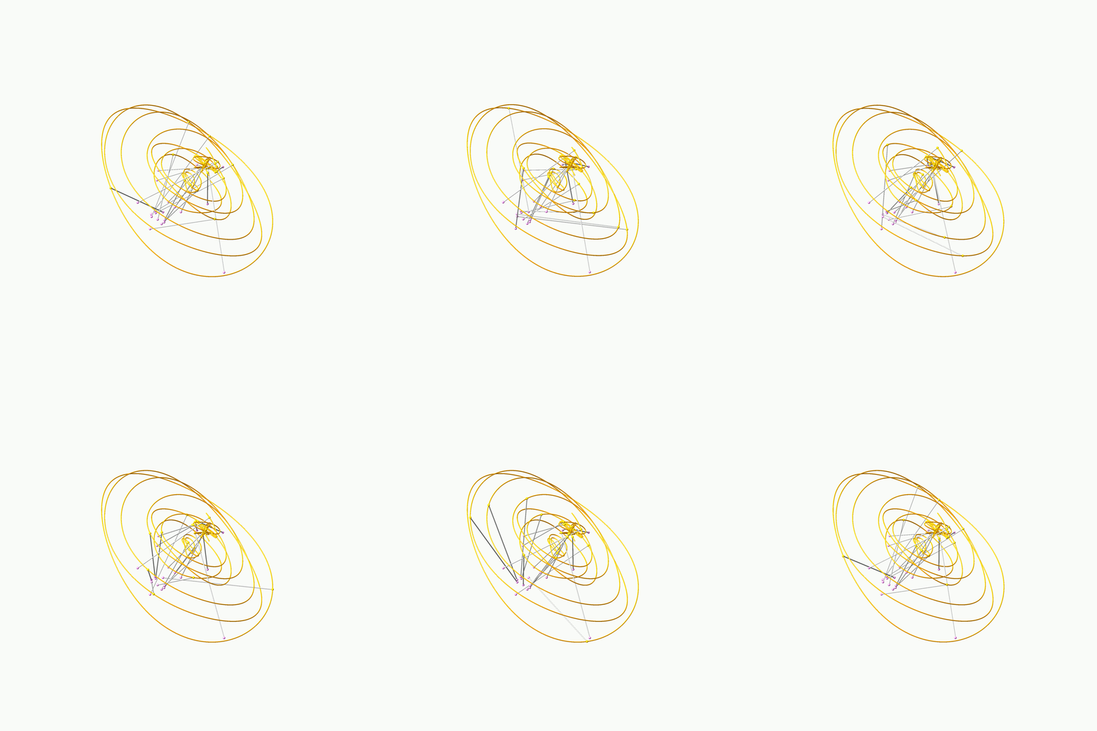
We apply a half-turn about a line through the point in direction to the platform. In the resulting initial position, which is illustrated in Figure 1, the squared leg lengths of the first six legs read as follows:
For this input data the self-motion consists of two components. The trajectories of the component which passes through the initial position are illustrated in Figures 3 and 4. In the latter figure also the associated basic surface is displayed. An animation of this line-symmetric self-motion can be downloaded from www.geometrie.tuwien.ac.at/nawratil/icosapod.gif.
We close the paper by mentioning two open questions that we find of interest:
- -
Starting from spectrahedra of type with one may construct mobile pods with , or legs: is it true that a general mobile pod with , or legs is line-symmetric? (It is known that have to be even numbers.)
- -
Identify all cases where more than points move on spheres during a line-symmetric motion; i.e. (a) 1-dim, (b) 2-dim or even (c) 3-dim set of points with spherical trajectories. Case (c) is completely known due to Bricard [Bri06], but cases (a) and (b) are still open. Examples for both cases are known (cf. Section 1.2.2 and [Bor08, Bri06, Kra37a, Naw15]).
Acknowledgments
The first and third-named author’s research is supported by the Austrian Science Fund (FWF): W1214-N15/DK9 and P26607 - “Algebraic Methods in Kinematics: Motion Factorisation and Bond Theory”. The second-named author’s research is funded by the Austrian Science Fund (FWF): P24927-N25 - “Stewart-Gough platforms with self-motions”.
References
- [Bor08] E. Borel, Mémoire sur les déplacements à trajectoires sphériques, Mémoire présenteés par divers savants à l’Académie des Sciences de l’Institut National de France 33 (1908), no. 1, 1–128.
- [BR79] O. Bottema and B. Roth, Theoretical Kinematics, Applied Mathematics and Mechanics, North-Holland Publishing Company, Amsterdam, 1979.
- [Bri01] R. Bricard, Sur une propriété du cylindroïde, Bull. Soc. Math. France 29 (1901), 18–21.
- [Bri06] by same author, Mémoire sur les déplacements à trajectoires sphériques, Journal de École Polytechnique(2) 11 (1906), 1–96.
- [DI11] A. Degtyarev and I. Itenberg, On real determinantal quartics, Proceedings of the Gökova Geometry-Topology Conference 2010, Int. Press, Somerville, MA, 2011, pp. 110–128.
- [Dup01] E. Duporcq, Sur un remarquable déplacement à deux paramétres, Bull. Soc. Math. France 29 (1901), 1–4.
- [GNS15a] M. Gallet, G. Nawratil, and J. Schicho, Bond theory for pentapods and hexapods, J. Geom. 106 (2015), 211–228.
- [GNS15b] by same author, Erratum to Möbius photogrammetry, J. Geom. 106 (2015), no. 3, 441–442.
- [GNS15c] by same author, Möbius photogrammetry, J. Geom. 106 (2015), no. 3, 421–439.
- [GS09] F. Geiss and F.-O. Schreyer, A family of exceptional Stewart-Gough mechanisms of genus 7, Interactions of Classical and Numerical Algebraic Geometry (Daniel Bates, GianMario Besana, Sandra Di Rocco, and Charles W. Wampler, eds.), Contemporary Mathematics, vol. 496, American Mathematical Society, 2009, pp. 221–234.
- [Ham11] M. Hamann, Line-symmetric motions with respect to reguli, Mech. Mach. Theory 46 (2011), no. 7, 960–974.
- [Har95] D. Hartmann, Singular Stewart-Gough platforms, Master’s thesis, Department of Mechanical Engineering, McGill University, Montreal, Canada, 1995.
- [HK02] M. Husty and A. Karger, Self motions of Stewart-Gough platforms, an overview, Proceedings of the workshop on fundamental issues and future research directions for parallel mechanisms and manipulators (Quebec City, Canada), 2002.
- [Hus00] M. Husty, E. Borel’s and R. Bricard’s papers on displacements with spherical paths and their relevance to self-motions of parallel manipulators, International Symposium on History of Machines and Mechanisms - Proceedings HMM 2000 (Marco Ceccarelli, ed.), Kluwer, 2000, pp. 163–172.
- [HZM94] M. Husty and P. Zsombor-Murray, A special type of singular Stewart Gough platform, Advances in Robot Kinematics and Computational Geometry (Jadran Lenarcic and Bahram Ravani, eds.), Kluwer, 1994, pp. 439–449.
- [Inn95] C. Innocenti, Polynomial solution of the spatial Burmester problem, J. Mech. Des. 117 (1995), no. 1, 64–68.
- [Kar03] A. Karger, Architecture singular planar parallel manipulators, Mech. Mach. Theory 38 (2003), no. 11, 1149–1164.
- [Kar08a] by same author, New self-motions of parallel manipulators, Advances in Robot Kinematics - Analysis and Design (Jadran Lenarcic and Philippe Wenger, eds.), Springer, 2008, pp. 275–282.
- [Kar08b] by same author, Self-motions of Stewart-Gough platform, Comput. Aided Geom. Design 25 (2008), no. 9, 775–783.
- [KH98] A. Karger and M. Husty, Classification of all self-motions of the original Stewart-Gough platform, Comput.-Aided Des. 30 (1998), no. 3, 205–215.
- [Kra37a] J. Krames, Die Borel-Bricard-Bewegung mit punktweise gekoppelten orthogonalen Hyperoloiden (Über symmetrische Schrotungen VI), Monatsheft für Mathematik und Physik 46 (1937), 172 –195.
- [Kra37b] by same author, Über Fußpunktkurven von Regelflächen und eine besondere Klasse von Raumbewegungen (Über symmetrische Schrotungen I), Monatsh. Math. Phys. 45 (1937), 394 –406.
- [Kra37c] by same author, Zur Bricardschen Bewegung, deren sämtliche Bahnkurven auf Kugeln liegen (Über symmetrische Schrotungen II), Monatsh. Math. Phys. 45 (1937), 407–417.
- [Kra37d] by same author, Zur Geometrie des Bennett’schen Mechanismus (Über symmetrische Schrotungen V), Sitzungsberichte d. österr. Akad. d. Wiss. math.-nw. Kl., Abt. IIa 146 (1937), 159–173.
- [Naw11a] G. Nawratil, Basic result on type II DM self-motions of planar Stewart Gough platforms, Mechanisms, Transmissions and Applications (Erwin-Christian Lovasz and Burkhard Corves, eds.), Springer, 2011, pp. 235–244.
- [Naw11b] by same author, Planar Stewart Gough platforms with a type II DM self-motion, J. Geom. 102 (2011), no. 1, 149–169.
- [Naw12] by same author, Necessary conditions for type II DM self-motions of planar Stewart Gough platforms, J. Geom. Graph. 16 (2012), no. 2, 139–151.
- [Naw13] by same author, Types of self-motions of planar Stewart Gough platforms, Meccanica 48 (2013), no. 5, 1177–1190.
- [Naw14a] by same author, Introducing the theory of bonds for Stewart Gough platforms with self-motions, J. Mechanisms Robotics 6 (2014), no. 1, 011004.
- [Naw14b] by same author, On the Self-Mobility of Point-Symmetric Hexapods, Symmetry 6 (2014), no. 4, 954–974.
- [Naw15] by same author, On the line-symmetry of self-motions of pentapods with linear platform, submitted [arXiv:1510.03567], 2015.
- [NS15] G. Nawratil and J. Schicho, Pentapods with Mobility 2, J. Mechanisms Robotics 7 (2015), no. 3, 031016.
- [NS16] by same author, Addendum to Pentapods with Mobility 2, [arXiv:1602.00932], 2016.
- [ORSV15] J. C. Ottem, K. Ranestad, B. Sturmfels, and C. Vinzant, Quartic spectrahedra, Math. Program. 151 (2015), no. 2, Ser. B, 585–612.
- [RM98] O. Röschel and S. Mick, Characterisation of architecturally shaky platforms, Advances in Robot Kinematics - Analysis and Control (Jadran Lenarcic and Manfred Husty, eds.), Kluwer, 1998, pp. 465–474.
- [Rot67] B. Roth, The kinematics of motion through finitely separated positions, J. Appl. Mech. 34 (1967), no. 3, 591–598.
- [Sch86] A. Schoenflies, Geometrie der Bewegung in synthetischer Darstellung, B.G. Teubner, Leipzig, 1886.
- [Sel13] J. M. Selig, On the geometry of the homogeneous representation for the group of proper rigid-body displacements, Rom. J. Tech. Sci. Appl. Mech. 58 (2013), no. 1-2, 153–176.
- [SH11] J. M. Selig and M. Husty, Half-turns and line symmetric motions, Mech. Mach. Theory 46 (2011), no. 2, 156–167.
- [SSW14] B. Schulze, A. Sljoka, and W. Whiteley, How does symmetry impact the flexibility of proteins?, Philos. Trans. R. Soc. Lond. Ser. A Math. Phys. Eng. Sci. 372 (2014), no. 2008, 20120041, 20. MR 3158333
- [Töl75] J. Tölke, Elementare Kennzeichnungen der symmetrischen Schrotung, Manuscripta Math. 15 (1975), no. 4, 309–321.
- [WW87] N. White and W. Whiteley, The algebraic geometry of motions of bar-and-body frameworks, SIAM J. Algebraic Discrete Methods 8 (1987), no. 1, 1–32. MR 872054