Properties of Robinson–Trautman solution with scalar hair
Abstract
An explicit Robinson–Trautman solution with minimally coupled free scalar field was derived and analyzed recently. It was shown that this solution possesses a curvature singularity which is initially naked but later enveloped by a horizon. However, this study concentrated on the general branch of the solution where all free constants are nonzero. Interesting special cases arise when some of the parameters are set to zero. In most of these cases the scalar field is still present. One of the cases is a static solution which represents a parametric limit of the Janis–Newman–Winicour scalar field spacetime. Additionally, we provide a calculation of the Bondi mass which clarifies the interpretation of the general solution. Finally, by a complex rotation of a parameter describing the strength of the scalar field we obtain a dynamical wormhole solution.
Keywords:
exact solution, black hole, scalar fieldpacs
04.20.Jb, 04.70.BwI Introduction
The Robinson–Trautman family of spacetimes contains nonsymmetric dynamical generalizations of several important solutions to the Einstein field equations — e.g., Schwarzschild and Vaydia solutions or the C-metric. Notably, these solutions generally contain gravitational waves and offer the possibility to study the evolution of initial generic data towards a final stationary situation. This family is defined by the presence of a nontwisting, nonshearing, and expanding null geodesic congruence.
Recently, we presented a Robinson–Trautman solution minimally coupled to a free massless scalar field [1] (a broader overview of the standard Robinson-Trautman solutions with many references can be found there). In this case, it was not possible to use the original form of the Robinson-Trautman metric which admits only pure radiation and the Maxwell field stress energy tensor aligned with the principal null direction or a cosmological constant. The reason was that the scalar field wave equation can not be satisfied for a scalar field whose gradient is aligned. The scalar field had to become non-aligned and the Robinson–Trautman metric had to be generalized to accommodate a broader class of energy-momentum tensors. Complete classification of such geometries including general forms of the curvature tensors is shown in [2].
To help us with the interpretation of our solution we compute the Bondi mass [3] which is the most suitable description of the energy content of the spacetime for the Robinson-Trautman class and was used in this context previously (see, e.g., [4] for the vacuum case computation by means of a conformal factor). We use the definition based on an asymptotic twistor equation adapted to a massless scalar field in [5]. The computation confirms the expectation based on an asymptotic form of the solution. Namely, the energy content of the spacetime is completely determined by a scalar field and there is no contribution of a Schwarzschild-type “mass”.
Next, we show the specific subcases which are all spherically symmetric and we connect them with previously analyzed solutions. This brings a certain degree of justification for considering the whole class as physically relevant.
Finally, inspired by a relation between a static subcase of our solution and a simple wormhole spacetime we analyze a wormhole version of the general Robinson–Trautman solution with a scalar field. Unlike the original solution, the wormhole version naturally does not satisfy any energy conditions and thus is not very physical. On the other hand, it provides a dynamical wormhole which gets created and then disappears while having surprising asymptotic behavior which is connected to the Kundt class. This family of solutions to the Einstein equations is closely related to the Robinson–Trautman geometry and is defined by the presence of a nontwisting, nonshearing, but (unlike Robinson–Trautman) nonexpanding null geodesic congruence. Most important members of this family are exact radiative spacetimes which generalize simple planar gravitational waves (e.g. pp-waves).
II Vacuum Robinson–Trautman metric and field equation
First, let us review the standard Robinson–Trautman solution for comparison and reference.
The vacuum Robinson–Trautman spacetime (possibly with a cosmological constant ) can be described by the line element [6, 7, 8, 9]
| (1) |
where ,
| (2) |
The metric generally contains two functions, and . The function might be set to a constant by suitable coordinate transformation [8, 9] and we consider this to be fulfilled for the coordinates of (1). The Einstein equations then reduce to a single nonlinear PDE — the Robinson–Trautman equation
| (3) |
These spacetimes are then generally of algebraic type II.
As required by the definition of the Robinson–Trautman family the spacetime admits a geodesic, shearfree, twistfree and expanding null congruence generated by with being an affine parameter along this congruence, is a retarded time and hypersurfaces are null. Spatial coordinates span a transversal 2-space which has the Gaussian curvature (for )
| (4) |
For general and , the Gaussian curvature is so that, as , these 2-spaces become locally flat. As usual we will assume that the transversal 2-spaces are compact and connected which leads to a subclass that contains the Schwarzschild solution (considering vanishing cosmological constant for simplicity) corresponding to (consistent with a spherical symmetry). This subclass thus represents its generalization to a nonsymmetric dynamical situation.
For analysis of the Robinson–Trautman equation (3) it is useful to introduce the following parametrization
| (5) |
where is a function on a 2-sphere , corresponding to (such choice gives ). By a rigorous analysis of the equation (3) together with the decomposition (5) Chruściel [10, 11] proved that, for an arbitrary, sufficiently smooth initial data on an initial hypersurface , the Robinson–Trautman type II vacuum spacetimes (1) exist globally for all . Moreover, they asymptotically converge to the Schwarzschild–(anti-)de Sitter metric with the corresponding mass and the cosmological constant as . This convergence is exponentially fast since behaves asymptotically as
| (6) |
where are smooth functions of the spatial coordinates . For large retarded times , the function given by (5) exponentially approaches which describes the corresponding spherically symmetric solution.
There is a closely related family of exact solutions possessing a null congruence which is nonexpanding (unlike in the case of Robinson–Trautman class), but still nontwisting and nonshearing — namely the Kundt family [12, 13]. The general line element can be given in the form [8, 9] (we use the same coordinate labels as in the Robinson–Trautman case to stress the similarities and differences)
| (7) | |||||
with being functions of all the coordinates. Note that the coordinate is absent from the transversal part of this metric which is given by the last two terms of (7) (compare with the Robinson–Trautman metric (1)). This directly leads to the privileged null congruence being nonexpanding. As we will see in the section VII this solution is closely related to an asymptotic state of the Robinson–Trautman geometry with an imaginary scalar field.
III Robinson–Trautman solution coupled to a scalar field
The Robinson–Trautman solution generalized to accommodate a scalar field is given in the following form [1]
| (8) | |||||
The scalar field is assumed to be a function of and only (). The dependence on means that the scalar field is not aligned (with respect to the direction given by its gradient). From the Einstein equations and the field equation for the scalar field
| (9) |
(where is a standard d’Alembert operator for our metric (8)) we obtained [1] the following expressions for unknown metric functions and the scalar field
| (10) | |||||
with this constraint between the constants appearing above
| (11) |
Unlike the case of the vacuum Robinson–Trautman spacetime (1) one needs to solve three Einstein equations with nontrivial right-hand side given by the stress energy tensor of the scalar field. The relation corresponding to the original Robinson–Trautman equation (3) is now transformed into
| (12) |
One can recognize double Laplacian in the last term on the left-hand side (note the expression for in (10)) and the second term of (3) has its analog at the beginning of the second line of (12). The main reason for the difference between the vacuum (1) and the scalar field (8) case is an incompatible separation of variables for the metric function standing in front of the spatial part . In the vacuum case the dependence on coordinates is split into and while in the scalar field case it is and . Additionally, the scalar field case has more nontrivial Einstein equations and also the scalar field equation to satisfy. This led to a solution which is more explicit rather than being left unintegrated as usual for the vacuum Robinson–Trautman metric where it is possible to prove the existence of a solution for the single Robinson–Trautman PDE (3). Although both the vacuum (even with pure radiation) and the scalar field Robinson–Trautman solutions are of algebraic type II (see Appendix) the Ricci (or Segre) type is different and most importantly the scalar field is not aligned with the principle direction of the Weyl tensor.
In the previous study [1] only a situation in which the constants satisfy was studied and the position of a curvature singularity and the existence of horizons was analyzed. Namely, it was shown that the singularity seems initially naked and only later it gets covered by the horizon. The asymptotic behavior of the metric was only hinted at in the original paper and since it shares its form with the special cases investigated later we will first derive the metric form when .
IV Asymptotic behavior
To arrive at the asymptotic form of the general metric 8 when goes to infinity one first notes that
| (13) |
for large values of when parameter is nonzero in the solution (10). Combining functions and together
| (14) |
it is easy to see that
where . Moreover, noting that
one can express another metric function in a familiar form
Collecting these pieces together we arrive at the metric
| (15) | |||||
which is exactly of the original Robinson–Trautman form (1) when and . So in the asymptotic region the generalized form of the Robinson–Trautman metric evolves into a standard one with vanishing mass parameter and without cosmological constant. Such solutions belong to algebraic type N subclass of the original Robinson–Trautman spacetimes [8, 9] and contain (apart from a trivial flat solution) radiative solutions possessing singularity for certain values of on each wave-surface. These combine into singular lines in the spacetime. As noted in [1] and repeated in appendix, the scalar field family of the Robinson–Trautman type does not contain these undesirable nontrivial type N solutions and therefore the final asymptotic state is just a flat spacetime (consistent with the vanishing scalar field in the asymptotic region). The specific reason for the absence of type N solutions with singular lines is the separated form of (14) which is the result of the selected form of the metric (8).
Note, that the approach to the final asymptotic state differs from the vacuum case. In the vacuum case the behavior is described by a simple exponential (3) while for the scalar field case the exponential depends quadratically on the retarded time (see (14) and (10)) provided . In this case the solution with a scalar field can additionally be extended to a negative infinite retarded time unlike in the vacuum case where the evolution generally blows up due to the parabolic nature of (3).
V Bondi mass
There are many possibilities how to compute a "mass" characterizing a given spacetime and its content. The definitions are built in such a way that they give expected results in situations where the correct answer seems obvious, like for the Schwarzschild solution with its mass parameter. When the spacetime geometry is suitable for a spacelike slicing the most natural one is either the ADM mass [14] (asymptotic flatness is usually assumed for the construction) or the Komar mass [15] (suitable for stationary spacetimes). But because of the standard formulation of the initial conditions for the Robinson-Trautman class (they are given on a null hypersurface) and the ensuing evolution in the retarded time direction we use the concept best suited to such a situation — the Bondi mass [3]. First, let us transform the original metric (8) by the following change of variables (inspired by [2]) and one redefinition of a function
| (16) |
In terms of the new variables and the function the scalar field becomes
| (17) |
(note the similarity with the potential of a finite rod in prolate ellipsoidal coordinates) and the metric simplifies into the following one
| (18) |
which gives an easier interpretation for the special cases in the next section and is also suitable to investigate the global evolution of the energy content in our spacetime. On the other hand, the coordinate cannot be integrated in a closed analytic form.
Now, we perform a conformal transformation of (18) so that the corresponding unphysical metric can be extended to the future null infinity in a standard way. Since the vector is normal to we select an appropriate conformal factor and introduce a new coordinate for convenience. The unphysical metric then reads
| (19) |
The coordinates of this metric represent the asymptotic Bondi coordinates near and the tetrad adapted to has the following form
| (20) | |||||
Since our spacetime contains a free massless scalar field we have to use a generalization of the standard covariant formula for calculation of the Bondi mass (based on a twistor equation) given in [5] (note the sign change due to a different signature convention)
| (21) |
In the above formula there appear the leading order terms of expansions of the standard Newman–Penrose quantities near the future null infinity. The integration is taken over a constant (or equivalently constant ) spatial sections of . Since our spacetime is shearfree the last term is identically zero while the first two combine to give
| (22) |
The surface area in the last expression is a finite positive constant and by inspecting the explicit form of we can see that asymptotically the Bondi mass smoothly decreases to zero. Also, the Bondi mass is completely given by the scalar field and is identically zero when the scalar field is switched off by putting . This confirms the previous result that our solution is related to the standard Robinson-Trautman geometry with vanishing mass parameter since otherwise the Bondi mass would contain additional contribution proportional to this parameter [4]. The natural interpretation of these results is that asymptotically the scalar field completely disappears being radiated away along .
VI Special cases
Now we focus on special values of the parameters determining the general solution. Specifically, we consider the simplified form of metric (18) for the analysis.
VI.1 Case
If we assume is zero it means that the scalar field vanishes and the condition for (11) (if it should remain finite) means that should approach zero as well which leads to . If we assume that the two-spaces spanned by are compact then the solution of the Laplace equation is necessarily a constant (the only harmonic functions on compact surfaces are constants). Since we assume the two-spaces to be regular its Gaussian curvature (determined by ) should be positive. Without loss of generality this constant can be chosen to be and we obtain a spherically symmetric situation, i.e.,
where
It is convenient to choose so the metric would be
which is obviously a flat spacetime and all the components of the Weyl spinor are zero.
As shown in the section IV the final state of the asymptotic evolution corresponds to a flat solution as well so the case of a vanishing scalar field just considered is the future attractor for the general solution in the class.
VI.2 Case
In this case, we have
or in other words, as in the previous case, is a constant and . The metric functions and become (note that now from (11))
so the original metric can be written in the following form
| (23) |
and all the Weyl scalars are zero except ,
Using the set of coordinates of the line element (18) the metric simplifies to this form
| (24) |
and the scalar field is retained in the form (17) with the function having a specific form derived below. Since , it is possible to solve the integral defining in the transformation (16) analytically, namely
| (25) |
where we can fix the constant of integration by demanding to obtain
Now we can write explicitly in terms of
| (26) |
This expression has moreover a reasonable limit for due to our choice of the constant . In terms of the new variables the scalar field becomes
| (27) |
where .
The Ricci scalar and the Kretschmann invariant are giving the position of a curvature singularity
| (28) | |||||
(using a specific form of the solution)
Obviously, the position given by the root of denominator changes linearly in . If one looks for an apparent or a trapping horizon possibly covering the singularity one arrives at the following equation for the horizon hypersurface (derived from the condition for vanishing expansion of a congruence orthogonal to a spherically symmetric section of the horizon hypersurface)
| (29) |
for convenience it is possible to write in terms of , namely
so 29 would be
| (30) |
At the same time we know that the singularity is at using (28).
By a simple coordinate transformation the metric (24) and the scalar field (27) can be shown to exactly correspond to the "nonstatic spherically symmetric massless scalar field" solution discussed by Roberts [16]. The presence of a horizon in this solution for certain values of parameters is briefly mentioned in [17] where more general spherically symmetric scalar fields with nontrivial potentials are discussed.
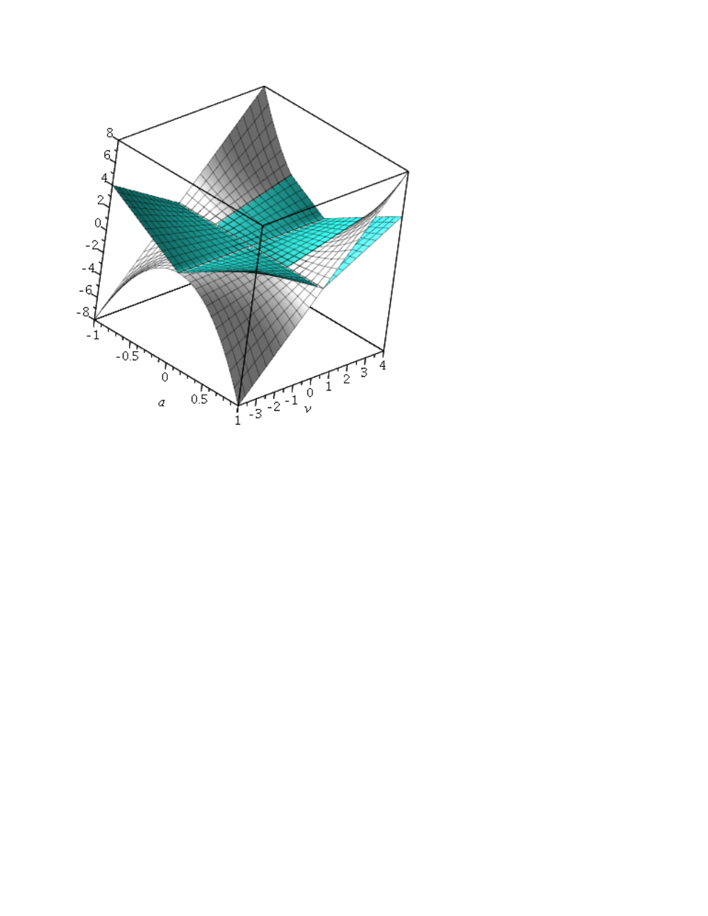
Introducing a reparametrization of the retarded time (notice the reversal of the time direction) and an auxiliary parameter we can understand the relative positions of the singularity and the horizon by plotting them as in the Figure 1. From the plot one sees that for the range of values the singularity is permanently naked while for the rest of the values the horizon is always present above the singularity for positive times .
One can immediately recognize that the above time reversal corresponds to changing from the retarded to the advanced time. If one would not reverse the time orientation one would start (for ) with singularity covered by a large horizon at negative time which would gradually shrink and merge with the singularity at time zero.
Note that now the original asymptotic value of translates according to (25) into or . There we immediately obtain and the scalar field (27) vanishes as well.
Interestingly, the Bondi mass now becomes proportional to the horizon position which indicates that in this spherically symmetric and dynamical case the Bondi mass (completely generated by the scalar field) plays the role similar to a variable mass in the Vaidya spacetime [18] in determining the horizon position.
VI.3 Case and
If we assume both and to be vanishing then becomes a constant
and the whole geometry becomes obviously static and spherically symmetric. In this case the line element (24) will simplify into
| (31) |
where and . Like in the previous case all the Weyl scalars are zero except which becomes
The scalar field is static as well
| (32) |
The Ricci scalar and the Kretschmann invariant are
| (33) |
One can easily see that the singularity is naked in this case, either directly from the metric (31) or by looking for marginally trapped surfaces. The Bondi mass is now vanishing which might seem surprising at first but it is exactly in accordance with the observation made in the previous case that related the Bondi mass to the horizon position — now the horizon is absent.
We can compare this static solution with the spherically symmetric static solution of Janis, Newmann and Winicour [19] in the coordinates given in [20, 21]
| (34) |
in which
| (35) |
and the scalar field is with the following relation between constants . One immediately sees that in the limit both the metric and the scalar field become identical (up to a trivial introduction of a null coordinate) to the static case given by (31) and (32).
Another connection to the previously studied spacetime can be found in the paper by Morris and Thorne [22] studying traversable wormholes. Namely, the toy model of a wormhole spacetime proposed there can be obtained from (31) by a simple complex transformation of a constant . This evidently means that the curvature scalars, e.g. (33), do not diverge anywhere and such a spacetime avoids the region with singularity by possessing a sphere with minimal areal radius which is nonzero. The scalar field becomes purely imaginary
so its stress energy tensor (being quadratic in ) violates energy conditions as expected for a wormhole. Note that we consider the change as a parametric transition in our original Einstein-scalar field system of equations which means that we use the same definition for the stress energy of a scalar field as in [1], namely the standard stress energy of a real scalar field. Of course the stress energy tensor of a true complex scalar field does not lead to such a violation of the energy conditions needed here.
When the scalar field is still vanishing in this case. The metric (31) is also evidently asymptotically flat. But the area of the spherical surfaces grows quadratically with the coordinate only far from the central region while close to the singularity it grows just linearly.
VII Imaginary scalar field
Inspired by Morris and Thorne [22] traversable wormholes and the simple relationship between their wormhole and our static solution 31, we apply a complex transformation to appropriate constant in the general solution (8). First, the scalar field becomes purely imaginary
| (36) |
and the stress energy tensor (being quadratic in ) violates all energy conditions. Second, the metric functions change accordingly
| (37) |
The metric sourced by a purely imaginary scalar field becomes
| (38) | |||||
The Ricci scalar is
| (39) |
and the Kretschmann invariant is again just its quadratic expression (using the specific form of the solution)
This means that the curvature scalars do not diverge anywhere and curvature singularities are absent in this spacetime.
If we compute the expansion of the congruence associated with the vector field
| (40) |
we can see that by continuing the coordinate to negative values (note that is now neither a curvature singularity nor a coordinate one) we have a spacetime where the congruence changes sign at . On the surface (which has a nonzero area) we not only have but also so it is a genuine wormhole throat satisfying the flare-out condition [23].

By looking at the Figure 2 one can recognize that the wormhole gets created only for a finite time close to the origin of coordinate . To show that this behavior is general (if we consider and ) one can easily compute that the expansion (40) has two extremes (a positive maximum and a negative minimum) for and . Combining this with the asymptotic behavior of the function (its explicit form (37) shows that it vanishes for both ) and the value of the expansion (40) for one immediately concludes that the throat structure analogous to that visualized in the Figure 2 is generic.
The asymptotic form of the metric (38) when goes to either positive or negative infinity is (note that now, unlike in the case of a real scalar field (10), the function asymptotically vanishes exponentially fast (37)),
and the scalar field 36 becomes a constant . The absence of any dependence on the coordinate in the two-dimensional metric defined on the subspace spanned by evidently means that the expansion of the congruence associated with the principal null vector is vanishing. So this limiting form of geometry belongs to the Kundt class (compare with (7) for vanishing and ) which is a nonexpanding counterpart of the Robinson–Trautman family.
The wormhole solution given above thus has genuine Robinson-Trautman behavior for finite times but asymptotically () transforms into a Kundt geometry. Specifically, it is related to a specific Kundt geometry coupled to a scalar waves (with ) discussed in [24].
The covariant (inverse trace) energy momentum tensor and its trace are zero asymptotically while the Weyl scalar and the Ricci coefficient are nonzero. This behavior just means that certain tetrad projections are nonvanishing in the limit due to the behavior of the tetrad vectors (or in other words the metric). On the other hand, inspecting the Ricci scalar (39) and the Kretschmann scalar in the asymptotic limit one can see that the mentioned divergences do not occur as a result of a strong curvature singularity presence. Nonzero and correspond to the Kundt-type gravitational and scalar waves both for the negative and positive infinite values of (see the form of the function ). One can interpret such a spacetime as containing a scalar wave (necessarily accompanied by a gravitational wave [24]) coming from infinity and focusing to create a wormhole which is not stable and gets again radiated away in the form of waves of both fields.
VIII Conclusion and final remarks
We have presented additional properties of the Robinson–Trautman spacetime with a minimally coupled free scalar field. This important class of nonsymmetric and dynamical spacetimes was endowed with a scalar field source only recently. Using the asymptotic form of the solution and the Bondi mass we have shown that the scalar field is the only contribution to the energy of this solution and the energy content of the solution decreases to zero at the infinite retarded time. Accordingly the geometry itself becomes flat asymptotically. We have compared the asymptotic behavior of the vacuum and the scalar field solutions. The original investigation of the vacuum solution asymptotics required extensive analysis carried out mainly by P. Chruściel and led to the Schwarzschild solution (or its variants) as the final asymptotic state.
Next, we have considered several special subcases of the general solution which all resulted in spherically symmetric situations. The case leads to a flat spacetime while and cases retain the scalar field. In the case both the scalar field and the geometry are dynamical while the case is completely static. We have shown that the dynamical case is similar to the Roberts solution while the static case corresponds to a limit of the Janis–Newmann–Winicour solution and is closely related to the simple version of the Morris–Thorne wormhole. This last correspondence led us to investigate a dynamical wormhole-type solution based on the general Robinson–Trautman spacetime with an imaginary scalar field. We showed that the wormhole throat appearance is generic and the asymptotics (both future and past one) is related to a subclass of the Kundt geometry with a scalar field. This provides a nontrivial connection between these two families of solutions to the Einstein equations on the level of a single spacetime.
Acknowledgements.
This work was supported by the grant GAČR No. 14-37086G.APPENDIX
We present the Weyl scalars for the general solution (8,10). Note that in the original paper [1] there are typos in the Weyl scalars presented there. Our preferred tetrad for determining the Weyl scalars of our solution is given by
| (42) | |||||
where is a complex unit. The Weyl spinor computed from this tetrad has only the following nonzero components
| (43) | |||||
As correctly computed in [1] the general algebraic type is II and in the special case of (constant positive Gaussian curvature of a compact two-space spanned by ) the algebraic type becomes D consistent with spherical symmetry. However, our family of solutions does not contain nontrivial type N radiative geometries that contain line singularities penetrating each wave surface.
References
- [1] T. Tahamtan and O. Svítek, Robinson-Trautman solution with scalar hair, Phys. Rev. D 91, 104032 (2015).
- [2] J. Podolský and R. Švarc, Algebraic classification of Robinson-Trautman spacetimes, in preparation
- [3] H.I. Bondi, Gravitational Waves in General Relativity, Nature 186, 535 (1960).
- [4] J. Tafel, Bondi mass in terms of the Penrose conformal factor, Class. Quantum Grav. 17, 4397 (2000).
- [5] J. Bičák, M. Scholtz and P. Tod, On asymptotically flat solutions of Einstein’s equations periodic in time: II. Spacetimes with scalar-field sources Class. Quantum Grav. 27, 175011 (2010).
- [6] I. Robinson and A. Trautman, Spherical Gravitational Waves, Phys. Rev. Lett. 4, 431 (1960).
- [7] I. Robinson and A. Trautman, Some Spherical Gravitational Waves in General Relativity, Proc. Roy. Soc. Lond. A265 , 463 (1962).
- [8] H. Stephani, D. Kramer, M.A.H. MacCallum, C. Hoenselaers and E. Herlt, Exact Solutions of the Einstein’s Field Equations, 2nd edn (CUPress Cambridge, 2002).
- [9] J.B. Griffiths and J. Podolský, Exact Space-Times in Einstein’s General Relativity, (Cambridge University Press, Cambridge, England, 2009).
- [10] P. T. Chruściel, Semi-global existence and convergence of solutions of the Robinson–Trautman (2-dimensional Calabi) equation, Commun. Math. Phys. 137, 289 (1991).
- [11] P. T. Chruściel, On the global structure of Robinson–Trautman space-times, Proc. Roy. Soc. Lond. A436, 299 (1992).
- [12] W. Kundt, The Plane-fronted Gravitational Waves, Z. Phys. 163 77 (1961).
- [13] W. Kundt, Exact Solutions of the Field Equations: Twist-Free Pure Radiation Fields, Proc. R. Soc. A 270 328 (1962).
- [14] R. Arnowitt, S. Deser, C. Misner, Dynamical Structure and Definition of Energy in General Relativity, Phys. Rev. 116 1322 (1959)
- [15] A. Komar, Positive-Definite Energy Density and Global Consequences for General Relativity, Phys. Rev. 129 1873 (1963).
- [16] M.D. Roberts, Scalar field counterexamples to the Cosmic Censorship Hypothesis, Gen. Rel. Grav. 21, 907 (1989).
- [17] X. Zhang and H. Lü, Exact black hole formation in asymptotically (A)dS and flat spacetimes, Phys. Lett. B 736, 455 (2014).
- [18] P.C. Vaidya, ‘Newtonian’ Time in General Relativity, Nature 171, 260 (1953).
- [19] A.I. Janis, E.T. Newman, and J. Winicour, Reality of the Schwarzschild singularity, Phys. Rev. Lett. 20, 878 (1968); M. Wyman, Static spherically symmetric scalar fields in general relativity, Phys. Rev. D 24, 839 (1981); I.Z. Fisher, Scalar mesostatic field with regard for gravitational effects, Zh. Eksp. Teor. Fiz. 18, 636 (1948), English translation: gr-qc/9911008.
- [20] A.I. Janis, D.C. Robinson, and J. Winicour, Comments on Einstein Scalar solutions, Phys. Rev. 186, 1729 (1969).
- [21] O. Svítek and T. Tahamtan, Ultrarelativistic boost with scalar field, Gen. Rel. Grav. 48, 22 (2016).
- [22] M.S. Morris and K.S. Thorne, Wormholes in spacetime and their use for interstellar travel: A tool for teaching general relativity, Am. J. Phys. 56, 395 (1987).
- [23] D. Hochberg and M. Visser, Dynamic wormholes, antitrapped surfaces, and energy conditions, Phys. Rev. D 58, 044021 (1998).
- [24] T. Tahamtan and O. Svítek, Kundt spacetimes minimally coupled to scalar field, arXiv:1505.01791.