Higher dimensional generalization of Buchdahl-Vaidya-Tikekar model for super compact star
Abstract
We obtain higher dimensional solutions for super compact star for the Buchdahl-Vaidya-Tikekar metric ansatz. In particular, Vaidya and Tikekar characterized the -geometry by a parameter, which is related to the sign of density gradient. It turns out that the key pressure isotropy equation continues to have the same Gauss form, and hence -dimensional solutions can be taken over to higher dimensions with satisfying the relation, where subscript refers to dimension of spacetime. Further is required else density would have undesirable feature of increasing with radius, and the equality indicates a constant density star described by the Schwarzschild interior solution. This means for a given , maximum dimension could only be , else will turn negative.
Keywords:
Higher dimensions; Einstein equations; Compact-super dense stars, hypergeometric functionspacs
04.20.Jb, 04.70.Bw, 04.40.NrI Introduction
There exists a vast literature on relativistic models for a star interior. The simplest and the oldest one is the constant density sphere described by Schwarzschild interior solution, and its universality for higher dimensions as well as for Lovelock gravity has also been established [1]. Another interesting fluid solution is isothermal sphere with a linear equation of state where is dimension of spacetime. It turns out that it also has universal solution for pure Lovelock (for which action and the equation of motion has only one term corresponding to , the degree of Lovelock action) gravity [2]. The former has undesirable feature of sound velocity being infinite, yet it accords to typical star interior parameters and overall behaviour while for the latter density is singular at the center though mass goes to zero, and it describes a relaxed equilibrium state of distribution without compact boundary. It could very well approximate a star or galaxy cluster. A physically reasonable distribution with a finite boundary lies between these two extremes.
There is a fairly general metric ansatz due to Buchdahl [3] that covers almost all interesting solutions. Vaidya and Tikekar [4] particularized Buchdahl ansatz by giving it a geometric meaning. They envisioned that -hypersurface is embedded in dimensional spheroid rather than sphere, and it is characterized by a dimensionless parameter , a measure of deviation from sphericity. Interestingly it turns out that sign of this parameter is also associated with density gradient. That is for gradient to be non-positive, must be non-negative and gives constant density. This indicates for a given mass or radius, star is densest when density is constant.
The point to be appreciated is that besides sphere and spheroid one can explore various topologies and see whether they accord to some meaningful physical distributions? For instance, if we consider a torus instead of spheroid, then we will write
| (1) |
where is distance from torus center to tube center and is tube radius. This will lead to the metric,
describing a fluid distribution with diverging density at center. It is therefore not physically acceptable.
Vaidya and Tikekar obtained solution for the case of [4] and the most general solution for integer values of was obtained by Mukherjee, Paul and Dadhich [5]. It may be noted that this metric ansatz is particularly suited for describing compact objects like neutron stars [6]. In this paper we wish to extend Buchdahl-Vaidya-Tikekar (BVT) model for compact star to higher dimensions. It turns out that the key pressure isotropy equation has the same Gauss form in higher dimensions as well. Hence -dimensional solutions could be carried over to higher dimensions with appropriately redefining the parameter which satisfies the relation where subscript indicates spacetime dimension. It may however be noted that though the solution is the same yet distribution is not entirely identical because density and pressure depend upon the parameter which is different for different . For a given , there would be a spectrum of values for different which has a cut-off at when representing uniform density.
There is also fairly large literature on star interior solution in higher dimensions, we give some representative references [7, 8, 9, 10, 11, 12, 13]. We have here studied how -dimensional solution could be taken over to appropriate higher dimensions in BVT metric ansatz. The paper is organized as follows: In the next section we write BVT metric and set up the equations for perfect fluid distribution. In Sec 3, we discuss the generalized higher dimensional solutions followed by discussion of their physical features.We end up with a discussion.
II Metric and Einstein equations
Let us begin with the general static spherically symmetric metric in the –dimensional spacetime,
| (2) |
Substituting the metric in the Einstein equation for a perfect fluid distribution, we obtain density and pressure (see for instance, Ref. [1] with ) as
| (3) |
| (4) |
and the pressure isotropy equation is given by
| (5) |
By writing , we rewrite the above equation
| (6) |
The Buchdahl ansatz [3] prescribes
| (7) |
with , which was particularized by Vaidya and Tikekar [4] to write
| (8) |
where . Now density reads as follows:
| (9) |
Clearly for density to be positive. For physical reasonableness, density gradient must be negative or zero,
| (10) |
This requires . The physical requirement of density decreasing with radius constrains the nature of -geometry or deviation from sphericity parameter cannot be negative.
Putting in the metric ansatz, the pressure isotropy equation takes the form
| (11) |
We further, as in Ref. [4], transform to
| (12) |
then Eqn (6) becomes
| (13) |
The only difference with the expression given in [4] is the factor in the last term of Eqn (13). This second order equation has two singular regular points in and we can write the solution around as in:[4]
| (14) |
where now coefficients are determined in terms of and , the two arbitrary constants of integration, as
| (15) |
Here even and odd coefficients are given respectively in terms of and . In the two tables below we give for explicitly even and odd coefficients, and they are:
| m | ||
|---|---|---|
| 0 | ||
| 2 | ||
| 4 | ||
| 6 |
| m | ||
|---|---|---|
| 1 | ||
| 3 | ||
| 5 | ||
| 7 |
From Eqn (15) it is clear that corresponding to a value for , the solution is the same for some in dimension. The general relation is
| (16) |
where subscript refers to dimension of spacetime. The solution is the same with replaced. This means there exists a higher dimensional fluid compact star with the same solution corresponding to every dimensional solution with proper value as given by the above relation. Note that coefficients of the corresponding series will be the same in terms of constants and .
Let us now consider some particular cases. For , which means six dimensional fluid sphere is of constant density. For , will turn negative and thereby implying density gradient being positive and hence untenable. For a given , the upper bound for dimension , else which is not physically admissible. Thus for , is only possible while for there could be respectively corresponding to , and so on. Uniform density marks the limiting case of maximum density and once that is reached, one cannot go any further in .
Here we have taken but that is not necessary, it can be any positive value. Uniform density sphere has the universal solution in the Schwarzschild interior metric irrespective of dimension of spacetime as well as Einstein or Lovelock gravity theory [1].
To gain some more insight let us recall the Vaidya-Tikekar construction [4]. We consider a spheroidal hypersurface in -Euclidean space defined by
| (17) |
which will generate the metric
| (18) |
where
| (19) |
Now the relation (16) can be written in the equivalent form, as:
| (20) |
This brings out how spheroidal parameters are related in the two cases.
Note that to obtain a polynomical solution instead of a series in Eqn (13), the coefficient must vanish. For this condition implies , where . Generalization of this simple rule in the case of Eqn (13) for a generic dimension leads to the requirement , which should have solution for positive integer number and . This shows there is a richer structure in higher dimensions 11 1 Other reformulation is that: for the finite series will be for , here , from where follows, that for any ; for for any where is an according integer such as, that is an integer positive number.
III The Solution
As in [5], a general solution for is given in terms of the Gegenbauer functions while in [3] it is expressed as the hypergeometric functions. By redefining variable, we can also write our solution in a more general form using hypergeometric functions, which would also include Gegenbauer functions as a particular case. Note that the equation (13), obtained for a spacetime of arbitrary dimension , can be transformed to a Gauss type differential equation [15], by a simple redefinition of the variable, : . Then we can transform Eqn. (13) to the standard form of the Gauss differential equation, written as:[16]
| (21) |
and the solution can be expressed as
| (22) |
where and are an arbitrary integration constants, and is the Gauss hypergeometric function in the usual notation [16].
The Gauss hypergeometric function has the following parameters :
| (23) |
where . Recall the parameter is restricted to be non-negative, . Thus we have the solution in closed form in terms of the Gauss hypergeometric functions 22 2 here also .
It is obvious, that Eqn. (21) has two singular points 33 3 we don’t consider here the singularity at , and they are . Near , the solution takes the form
| (24) |
while for near , it reads as
| (25) |
We have given above in Eqns (9) and (4) the expressions for density and pressure. Let us consider
| (26) |
and we can write
| (27) |
To determine the unknown integration constants and we should match and functions in (2) with the exterior Schwarzschild solution,
| (28) |
where
| (29) |
Here is higher dimensional gravitation constant and is mass of star [17],[18]. The star boundary is defined by vanishing pressure, on the surface and we determine the free parameters as
where
The variable is expressed in terms of 44 4 for we have :
where is the star radius. For , density and pressure are given by
| (30) |
To compute the derivatives and we can use some properties of the Gauss hypergeometric functions and obtain for them the following expressions:
| (31) |
| (32) |
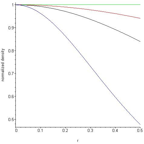
In Figs. 1 and 2 we plot normalized density, and pressure for the two cases . Since pressure value as well as its variation is very small for the case of constant density for , its blow up is shown in Fig 3. Note that for , we have corresponding respectively to , while for it is and . Clearly density variation slows down as dimension increases until constant density is reached (Fig 1). In Fig 2 we see that central pressure decreases with increasing dimension and so does its variation. For constant density distribution pressure has very small value and so is its variation (Fig 3). It should be noted that for the case , the variable (14) turns vacuous and hence it should be considered separately from the isotropy equation (11) itself.


Using the expression for the density in Eqn (3), let us introduce a new function, defined as:
| (33) |
In terms of this function we can express the variable, like which simply looks as:
| (34) |
After these redefinitions of variables, the equation of state, (EoS), can be written using the change of variables in the form and the speed of sound , where
The equation of state is given by
| (35) |
where is defined as:
| (36) |
The speed of sound is written as
| (37) |
here . We have thus obtained the equation of state and sound velocity involving parameters.
IV Discussion
The main point we wish to make is that character of the key pressure isotropy equation for the BVT ansatz for the static spherically symmetric metric remains unaltered when we go higher in dimension. That means solution would always have the same form. Further it turns out that corresponding to every -dimensional solution with a given , there exists a similar solution (since is different in two cases, solution would not be the same but similar) in higher dimension with corresponding . The -dimensional solution is carried over to higher dimensions but it represents different distribution. That is, the same metric with different value describes different distributions in different dimension. For a given , we can only go upto dimension when vanishes indicating constant density. Beyond that would turn negative implying density increasing with radius which is not physically tenable. Note that for , the only possible solution is constant density star in dimension with while for we could have solutions for with respectively. As increases decreases to zero marking the cutoff for .
Since density gradient is always required to be negative, star is densest when density is constant implying infinite sound velocity. This is the limiting case in evolution of a static distribution in equilibrium, and it is always described by the Schwarzshild interior solution irrespective of spacetime dimension as well as gravitational theory, Einstein or Lovelock gravity [1]. Though there exists uniform density solution in any dimension with given by the Schwarzschild interior solution but that would not have a correspondence with solution unless . For the BVT ansatz, we have found a correspondence between dimensional solutions with their analogues in higher dimensions. For a given value of , there is a spectrum of values.
It is possible to generalize the metric ansatz to bring in rotation by considering -geometry being ellipsoidal. That would be very suitable for considering fluid distribution with rotation which is a very important open problem as there exists no interior metric for a rotating Kerr black hole. This may shed some new light and perhaps lead to some new insight. Another important question for further investigation is stability analysis of these higher dimensional solutions. These would be our concerns for future study.
Acknowledgements
AK and AM gratefully acknowledges IUCAA for the invitation and warm hospitality which facilitated this collaboration. Partial support for this work to AK was provided by Uzbekistan Foundation for Fundamental Research project F2-FA-F-116. Authors also express their thanks to R. Tikekar for the useful discussions and his interest in this work.
References
- [1] N. Dadhich, A. Molina and A. Khugaev,Phys. Rev. D81, 104026, (2010)
- [2] N Dadhich, S Hansraj, S Maharaj, Universality of isothermal fluid spheres in Lovelock gravity, arxiv:1510.07490
- [3] H. A. Buchdahl Phys. Rev.116, 1027 (1959) & Class. Quantum. Grav.1, 301 (1984)
- [4] P. C. Vaidya, Ramesh Tikekar,J. Astrophys. Astr.3, 325 (1982).
- [5] S. Mukherjee, B.C. Paul, and N. Dadhich, Class. Quantum Grav., 14, 3475, (1997).
- [6] H. Knutsen, Astrophys. Space Science 98, 207 (1984)
- [7] Koikawa T., Phys. Lett. A, 117 (1986) 279
- [8] Koikawa T. and Yoshimura M., Prog. Theor. Phys., 75 (1986) 977.
- [9] Krori K. D., Borgohain P. and Das K., Phys. Lett. A, 132 (1988) 321.
- [10] Krori K. D., Borgohain P. and Das K., Can. J. Phys., 67 (1989) 25.
- [11] Maharaj S. D. and Patel L. K. Nuovo Cimento B, 111, (1996) 1005
- [12] Patel L. K., Mehta N. P. and Maharaj S. D., Nuovo Cimento B, 112, (1997) 1037.
- [13] S. D. Maharaj, B. Chilambwe, S Hansraj, Phys. Rev. D91, 084049 (2015); arxiv:1512.08072
- [14] Iwao Sugai, The American Mathematical Monthly, v. 67, No 2, 134, (1960)
- [15] Morse P.M. and Feshbach H., Methods of Theoretical Physics, v.1, New-York: McGraw-Hill, p.782,(1953).
- [16] Slater L.J.,Generalized Hypergeometric Functions, Cambridge University Press, p274,(1966).
- [17] P. Kanti, T. Pappas and N. Pappas, arXiv: 1409.8664v1 [hep-th], 30 Sep., (2014)
- [18] F. Tangherlini, Nuovo Cimento, 27, 636, (1963)