Charge and spin dynamics driven by ultrashort extreme broadband pulses: a theory perspective

Andrey S. Moskalenko Email: andrey.moskalenko@uni-konstanz.de Affiliation: Institut für Physik, Martin-Luther-Universität Halle-Wittenberg, 06099 Halle, Germany Affiliation: Department of Physics and Center for Applied Photonics, University of Konstanz, 78457 Konstanz, Germany Zhen-Gang Zhu Email: zgzhu@ucas.ac.cn Affiliation: Institut für Physik, Martin-Luther-Universität Halle-Wittenberg, 06099 Halle, Germany Affiliation: School of Electronic, Electrical and Communication Engineering, University of Chinese Academy of Sciences, Beijing 100049, China Jamal Berakdar Thanks: Corresponding author Email: jamal.berakdar@physik.uni-halle.de Affiliation: Institut für Physik, Martin-Luther-Universität Halle-Wittenberg, 06099 Halle, Germany

August 24, 2026

Abstract

This article gives an overview on recent theoretical progress in controlling the charge and spin dynamics in low-dimensional electronic systems by means of ultrashort and ultrabroadband electromagnetic pulses. A particular focus is put on sub-cycle and single-cycle pulses and their utilization for coherent control. The discussion is mostly limited to cases where the pulse duration is shorter than the characteristic time scales associated with the involved spectral features of the excitations. The relevant current theoretical knowledge is presented in a coherent, pedagogic manner. We work out that the pulse action amounts in essence to a quantum map between the quantum states of the system at an appropriately chosen time moment during the pulse. The influence of a particular pulse shape on the post-pulse dynamics is reduced to several integral parameters entering the expression for the quantum map. The validity range of this reduction scheme for different strengths of the driving fields is established and discussed for particular nanostructures. Acting with a periodic pulse sequence, it is shown how the system can be steered to and largely maintained in predefined states. The conditions for this nonequilibrium sustainability are worked out by means of geometric phases, which are identified as the appropriate quantities to indicate quasistationarity of periodically driven quantum systems. Demonstrations are presented for the control of the charge, spin, and valley degrees of freedom in nanostructures on picosecond and subpicosecond time scales. The theory is illustrated with several applications to one-dimensional semiconductor quantum wires and superlattices, double quantum dots, semiconductor and graphene quantum rings. In the case of a periodic pulsed driving the influence of the relaxation and decoherence processes is included by utilizing the density matrix approach. The integrated and time-dependent spectra of the light emitted from the driven system deliver information on its spin-dependent dynamics. We review examples of such spectra of photons emitted from pulse-driven nanostructures as well as a possibility to characterize and control the light polarization on an ultrafast time scale. Furthermore, we consider the response of strongly correlated systems to short broadband pulses and show that this case bears a great potential to unveil high order correlations while they build up upon excitations.

Keywords:

Broadband pulses, light-matter interaction, half-cycle pulses, THz pulses, non-resonant driving, ultrafast dynamics in nanostructures, ultrafast spectroscopy, intraband transitions, ultrafast spin dynamics, dynamic geometric phases

pacs

78.67.-n, 71.70.Ej, 42.65.Re, 72.25.Fe

1 Introduction

Electromagnetic waves are omnipresent in modern society with a vast variety of applications ranging from TV, radio, and cell phones to high power lasers and ultra precision metrology. In scientific research, newly invented methods offer a wide range of pulse durations from nanoseconds, through picoseconds, femtoseconds to currently attoseconds [1, 2, 3] opening so new avenues for research to explore the time evolution in a desired spectral regime which has lead to landmark discoveries in physics and chemistry. The key point thereby is the exploitation of the light-matter interaction to steer the system in a controlled manner out of the equilibrium or to stabilize it in target states by irradiation with shaped electromagnetic waves. The study of the behavior of nonequilibrium quantum systems driven by short light pulses has evolved so, depending on the goals and applications, to diverse sub-branches such as photovoltaics [4, 5, 6, 7], optical, electro- and magnetooptical devices [8, 9, 10, 11, 12, 13] as well as efficient schemes for the control of chemical processes [14, 15, 16, 17, 18]. Particularly, the studies of nonequilibrium processes in nanostructures are fueled by the equally impressive progress in nanoscience allowing to fabricate and engineer structures with desired geometric and electronic properties and bringing them to real applications, e.g. as an efficient radiation emitter in a broad frequency range or parts in electronic circuits. From a theoretical point of view, the currently available nanostructures with well-defined and simple topology like quantum wells [19, 20], quantum rings [21, 22, 23, 24, 25, 26, 27, 28, 29, 30, 31], quantum dots [20, 32, 33, 34, 35], and quantum spheres [36, 37] are particularly appealing, as they allow for a clear understanding of their static and nonequilibrium behavior. Hence, our main focus will be on these structures. As for the driving electromagnetic fields, emphasis is put on the utilization of broadband ultrashort pulses because they offer efficient schemes for steering the nonequilibrium states of matter. There has been an enormous progress in the generation and design of ultrashort pulses allowing to control the duration, the shape, the strength, the polarization properties, the focusing, the repetition rates, as well as the spectral bandwidth [38, 39, 40, 41, 42, 43, 44, 45, 46, 47, 48, 49, 50, 51, 52, 53, 54, 55, 56, 1, 57, 58, 59, 60, 61, 62, 63, 64, 65]. The pulses which are in the focus of this review are briefly introduced and discussed in Section 2. Excitations by short electromagnetic pulses may proceed resonantly or non-resonantly. In the first case, the light frequency is selected as to match a certain quantum transitions in the system. A paradigm of resonant excitations are driven two-level systems [66]. For instance, the application of resonant circular polarized $\pi$ -pulses [ $\int\Omega_{\rm R}(t)\mbox{d}t=\pi$ , where $\Omega_{\rm R}(t)$ is the Rabi frequency] to quantum rings leads to a population transfer between the ring quantum states, provided the pulse duration is much shorter than the typical time scales of dissipative processes in the system. It was theoretically demonstrated how to generate nonequilibrium charge currents in semiconductor and molecular quantum rings with the help of an appropriate resonant excitation by light pulses [67, 31]. In another characteristic case of the $\pi/2$ -pulses applied to the same system, a rotating charge density is generated in the rings, additionally to the current, which is in this case smaller by a factor of two [30]. For quantum dots, the resonant excitation with short light pulses can lead to population inversion of confined exciton states, as it was demonstrated experimentally using $\pi$ -pulses [68]. The reduction of the light-matter interaction to transitions in driven two-level systems is based on the so-called “rotating wave” approximation. It is effective only if the pulse duration is long enough, on the order of ten wave cycles or longer, and the central frequency of the pulse exactly matches the frequency of the induced transition. The required number of wave cycles can be slightly reduced if the optimal control theory is implemented for the driving pulse [69]. The resonant excitation with few wave cycles seems to be inappropriate if the desired result of the excitation requires transitions between many levels of the driven system, which are generally not equidistantly spaced in energy. A predictable result may require application of a pulse sequence with different central frequencies [67], at the cost of much longer duration of such an excitation.

To stay with the example of a phase-coherent ring, if the driving field is non-resonant, and if its strength is sufficiently large, the states of the ring become dressed by the photon field [70, 71, 72]. If the field is circularly polarized, the degeneracy between the field-counter and anti-counter propagating ring states is lifted and a finite current emerges in the ring (in the presence of the field) [73]. The phase change associated with this break of symmetry goes, as usual for non-resonant effects, at least quadratically with the field strength and hence becomes important at higher intensities. On the other hand, at high intensities multiphoton processes or tunnelling in the electric field of the laser may also contribute substantially depending on the frequencies [74]. We deal in this work with a further kind of processes which are not really resonant but still may occur to the first order in the driving field. This is the case of a broadband pulse covering a large number of the system excitations [75]. An example of an ultrabroadband pulse is an asymmetric monocycle electromagnetic pulse, also called half-cycle pulse (HCP) [39, 40, 76, 77, 78, 79, 80, 52, 58]. The electric field of a linear polarized HCP performs a short and strong oscillation half-cycle followed by a long but much weaker tail of an opposite polarity. If the duration of the tail is much longer than the characteristic time scales of the excited system then its effect can be neglected. Such a pulse contains a broad band of frequencies, particularly with a decreasing pulse duration. If the pulse duration becomes significantly smaller than the characteristic time scales of the system under study, then the action of the HCP subsumes to an appropriate matching of the wave functions (or the density matrix if a many-body consideration of the system is required) before and just after the pulse application. This does not mean that the state after the pulse is in general an eigenstate, but usually a coherent state. Classically, the matching condition corresponds in fact to an instantaneous transfer of a momentum $\Delta p$ (a kick) to the system [81, 82, 83, 84, 85, 86, 87]. The transferred momentum is proportional to the pulse strength and its duration. For confined electrons, usually the momentum operator does not commute with the field-free Hamiltonian and hence the pulse-induced momentum shift generates a coherent state. Quantum mechanically, the wave function $\Psi(x,t)$ of a one-dimensional system subjected at the time moment $t=0$ to the action of a HCP obeys the matching condition $\Psi(x,t=0^{+})=\exp(i\Delta px/\hslash)\Psi(x,t=0^{-})$ . Here $t=0^{-}$ is the time moment just before the pulse and $t=0^{+}$ is right after it. This matching condition is the essence of the impulsive (or sudden) approximation (IA). The pulse-generated coherent state develops in the time after the pulse according to the original Hamiltonian. Below we work out the validity range of this stroboscopic evolution scenario. Terahertz (THz) HCPs and trains of HCPs were considered in the impulsive regime to orient polar molecules [85, 79, 88], to manipulate the populations and control the orbital motion of electrons in Rydberg states [76, 89, 77, 90, 91, 78, 83, 84, 87, 59, 92], and to steer the electronic density of ionized atoms and molecules on the attosecond time scale [93, 94, 95, 96].

Generally, the area of driven quantum systems is huge with a number of sub-branches depending on the type of driving, the system under consideration, and the intended goals. The focus of this review is on the theory of quantum dynamics driven by ultra broadband short pulses. To be more specific we discuss briefly in Section 2 the type of the appropriate experimental pulses and mention some methods of generating them. In Section 3 we discuss a general perturbation theory for the unitary evolution operator of a quantum system driven by ultrashort external pulsed fields, where the small parameter is the pulse duration. Such a development is important for the understanding of the approximation steps leading to the IA in the case of HCPs and determining its limits of validity. Apart from this, we discuss cases when a theory beyond the IA should be applied. The corresponding theoretical considerations can be found in literature [97, 85, 98, 99, 100, 93, 101] but a development of a consistent perturbation theory with the pulse duration as a small parameter was absent until recently when it was formulated for atoms excited by light pulses confined to a small and finite time range [102, 103]. We present here an alternative derivation which is suitable also for pulse-driven nanostructures and includes the natural case of short light pulses with decaying tails which are however not necessarily strictly confined to a finite time range. With this approach we get an approximative description of the action of ultrashort pulses of a general shape, e.g. also in the cases of single-cycle pulses and few-cycle pulses, as a map between the states of the driven system before and after the pulse. Further in Section 2, we concern ourselves with the limits of validity of such a treatment of the excitation process. Interestingly, the IA may remain valid in some range of parameters even when the entire unitary perturbation expansion in the pulse duration breaks down due to the increase of the pulse amplitude. In this regime of short but very strong (SVS) interactions the next order correction to the unitary evolution operator beyond the IA can be also found. We discuss implications of the IA, unitary perturbation theory and SVS result for general one-dimensional geometries and two-level systems. In last part of Section 2 these findings are used to describe driving by periodic trains of the pulses and characterize the resulting quantum dynamics. We describe conditions for the controlled periodicity and quasistationarity of the evolution.

Sections 4 and 5 introduce various applications of the developed theoretical methods for particular nanostructures. Here we start with the pulse-driven dynamics of electrons moving along a spatially-periodic potential energy landscape (mimicking semiconductor superlattices, or generally crystal lattices and superlattices). Indirect transitions and charge currents can be induced in unbiased structures on extremely short time scales [104]. These results are especially appealing in view of an impressive ongoing progress on ultrafast control of the electron dynamics in solids by strong light pulses [105, 106, 107, 108, 109, 110, 111]. The reviewed approach provides access to this dynamics in a different, complementary and so far unexplored regime with distinct and unique features. Further in Section 4, we discuss how the charge polarization can be induced in double quantum wells and controlled by periodic pulse trains [112, 113]. Then we switch our attention to the light-driven semiconductor quantum rings, where apart from the charge polarization dynamics also nonequilibrium charge currents can be induced by an appropriate sequence of two light pulses [114, 115, 11]. This dynamics can be influenced by a perpendicular magnetic flux piercing the semiconductor ring [116]. The induced polarization dynamics and current are subjects to decoherence and relaxation processes [117, 118]. The capability to model these processes allows to create schemes for the charge current switching and generation of local magnetic fields with a tunable time structure [117]. We show that if transferred to graphene quantum rings, these ideas suggest a way for an ultrafast generation of pure valley currents [119]. In Section 5, we concentrate our attention on the spin dynamics triggered by ultrashort light pulses in semiconductor quantum structures and discuss how the spin dynamics can be steered to generate spin dependent polarization, spin-polarized current, and pure spin currents in nanostructures [120, 120, 121, 122, 123]. Proposals for an optically driven spin field-effect transistor [124] and ultrafast spin filtering [125] are described.

Section 6 is devoted to the emission properties and their control associated with the dynamics of the pulse-driven nonequilibrium dynamics. Finally, in Section 7 we discuss briefly how short, broadband pulses can be utilized to explore many-body effects in correlated systems [126], finishing with a summary and concluding remarks.

2 Generation of short broadband pulses

While we mainly aim in this report at the theoretical aspects of the short-time dynamics triggered by broadband pulses, it is useful to briefly discuss the appropriate experimentally available pulses. In this review we consider a pulse to be short and call it also “ultrashort” if its duration is on the scale or smaller than the generic times of the involved transitions that is is reflected in a respective frequency range of the pulse. Thus, depending on the problem at hand a picosecond pulse might be short enough, as for instance for the case of intra conduction band excitations in micron-size, semiconductor-based quantum rings. Other processes may require femtosecond or sub-femtosecond pulses. Even the latter pulses became recently available. An example is shown in Fig. 1. The field transient was produced by synthesizing intense optical attosecond pulses in the visible and nearby spectral ranges [64]. In this scheme 1.1 to 4.6 eV wide-band pulses are divided by dichroic beam splitters into spectral bands and then each band is compressed and spatiotemporally superimposed to yield a pulse such as the one in Fig. 1. The intensity profile duration is approximately 380 as at FWHM. Moreover, the carrier-envelope phase of such field transients can be adjusted to produce “near-cosine” and “near-sine” waveforms [127]. Synthesized sub-cycle pulses in the mid-infrared which are suitable for our purposes were reported also in Ref. [128] and further references therein.

Refer to caption — Figure 1: Electric field of a femtosecond unipolar pulse produced via an attosecond light-field synthesizer. Reproduced from Ref. [64] with permission from NPG group.

There is a possibility to generate strong near-field pulses that may drive impulsively charge and spin dynamics in the THz regime by using plasmonic structures such as bullseye structures consisting of annular grooves [129]. A cross-sectional line diagram illustrating the setup is shown in Fig. 2 , which also includes the time-domain waveform and the amplitude spectra. In recent years there has been an enormous progress in designing and applying plasmonic structures for near-field THz generation ; we refer to Refs. [130, 131] and the references therein for further details on this topic.

Theory illustrations presented in the following sections employ mostly strong single- or sub-cycle THz pulses applied to systems with spectral features in the far-infrared range. In this context we will discuss in detail the ballistic charge and spin manipulation in mesoscopic rings and quantum wires. Although the dynamics of the molecular rotations is outside of the scope of the present review, it is important to note that the same excitation regime can be successfully realized in the case of orientation of polar molecules and alignment of nonpolar molecules (cf. the review article [132] and references therein). Apart from this, the pulses of this type were used to study the acceleration of carriers and postpulse dynamics in semiconductor heterostructures [133, 134].

Another method to generate the appropriate pulses is to use photoconductive (Auston) switches [135, 136]. The schematics is shown in Fig. 3: A semiconductor-based structure with short carrier lifetime, for instance GaAs or silicon on sapphire, is biased with tens of volts amounting to an electric field of few kV/cm acting across the photoconductive area (cf. Fig. 3). The switch is then electrically shortened by a femtosecond laser pulse with a frequency above the band gap of the biased semiconductor, resulting in the generation of free carriers and their following votage-induced acceleration. This process leads to an abrupt polarization change which goes along with the emission of a sub-picosecond, single-cycle coherent electromagnetic pulse that propagates along the electrodes and in free space with a polarization being predominantly along the bias field. The free-space pulses are time-asymmetric , as evident from the way they are generated (cf. Fig.3). Yet, the integral of the amplitude of the electric field that propagates in free-space over its full duration vanishes. The temporal asymmetry of these pulses is essential for a number of phenomena discussed in this review from the theory point of view, such as the impulsive driving of charge and spin. Relevant experimental demonstrations exist in the field of atomic physics and include the impulsive ionization and the controllable steering of wave packets in Rydberg states of atoms [76, 39, 137, 78, 138, 139, 92]. The formal theory behind this type of dynamics is reviewed in this work. For further discussions of the Auston-switch-type technique for generating pulses as well as for antenna geometries other than the one shown in Fig. 3 (such as interdigitated structures, bow-tie, and spiral antennas) we refer to the dedicated literature, for instance [140, 141, 142, 143].

Here we will be also concerned with high-field pulses triggering excitation processes which are strongly nonlinear in the field strength. Such pulses were accomplished by using miniaturized interdigitated metal-semiconductor-metal structures [144, 145] or by enlarging the photoconductive antenna area (up to cm) and increasing the bias voltage (up to several kV) leading to pulse energies in the range of $\mu$ J [76, 39] , which were demonstrated to cause field ionization of Rydberg states.

A further way to generate intense single-cycle THz pulses relies on nonlinear processes in gas plasmas subjected to an intense femtosecond laser [146, 147, 148]. As a gas ambient air, nitrogen or a noble gas were utilized. By this method THz pulses with frequency band extending up to 100 THz and supporting a sub-20-fs duration were reported [149]. Also optical rectification of conventional (relatively narrow-band) picosecond or femtosecond laser pulses [150, 151], in electro-optical materials like LiNbO₃ , ZnTe, GaP, or GaSe, under appropriate conditions can lead to ultrashort broadband THz pulses suitable for the aims of this work. A further promising route relies on novel metallic spintronic emitters, which produce femtosecond pulses covering the 1–30 THz range with flat spectral amplitude and phase [65].

3 Theoretical description of the unitary evolution

In this section we develop a systematic description and approximation schemes for the dynamics of an electronic quantum system driven by ultrashort pulses of electromagnetic radiation. Let us consider a general system described by the Hamiltonian $H_{0}$ which is subjected at $t=t_{1}$ to an electromagnetic pulse. The pulse duration is $\tau_{\mathrm{d}}$ . The system evolves without time-dependent external forces from a time moment $t_{0}$ before the pulse application. For brevity we may choose $t_{0}=0$ , i.e., the evolution involving external driving is prescribed by the operator $U(t,0)$ that satisfies the equation of motion

i\hslash\frac{\partial U(t,0)}{\partial t}=[H_{0}+V(t)]U(t,0)\;,

(1)

where $V(t)$ describes the coupling of the pulse to the system. For clarity of notation we do not explicitly indicate spatial coordinates, unless deemed necessary. To separate the field-free propagation before and after the pulse we write the evolution operator in the form ( $t>t_{1}$ ) [85, 100, 152]

U(t,0)=U_{0}(t,t_{1})\mathcal{U}(t,t_{1},0)U_{0}(t_{1},0)\;,

(2)

where $U_{0}(t,t^{\prime})\equiv U_{0}(t-t^{\prime})=\exp\left[-iH_{0}(t-t^{\prime})/\hslash\right]$ is the evolution operator of the unperturbed system in the time interval from $t^{\prime}$ to $t$ and $\mathcal{U}$ is yet to be determined. The unitarity of $U_{0}$ dictates that

\mathcal{U}(t,t_{1},0)=U_{0}^{{\dagger}}(t,t_{1})U(t,0)U_{0}^{{\dagger}}(t_{1},0)

(3)

applies. Inserting Eq. (3) into Eq. (1) we infer a relation for $\mathcal{U}(t,t_{1},t_{0})$ that can be written formally as

\mathcal{U}(t,t_{1},0)=\hat{\textrm{T}}\exp\left[\int_{-t_{1}}^{t-t_{1}}A(t^{\prime},t_{1},0)dt^{\prime}\right],

(4)

where

A(t,t_{1},0)=-\frac{i}{\hslash}e^{iH_{0}t/\hslash}V(t+t_{1})e^{-iH_{0}t/\hslash}

(5)

and $\hat{\textrm{T}}$ is the time-ordering operator. It was shown by Magnus [153] and thoroughly discussed and illustrated in following works [154, 155, 156] that Eq. (4) can be expressed in a form that does not involve time ordering by writing

\mathcal{U}(t,t_{1},0)=\exp\left[\Omega(t,t_{1},0)\right],

(6)

where

\Omega(t,t_{1},0)=\sum_{k=1}^{\infty}\Omega_{k}(t,t_{1},0)\;

(7)

with the first two terms of this Magnus expansion given by

	$\displaystyle\Omega_{1}(t,t_{1},0)$	$\displaystyle=$	$\displaystyle\int_{-t_{1}}^{t-t_{1}}\!\!dt^{\prime}\>A(t^{\prime},t_{1},0)\;,$		(8)
	$\displaystyle\Omega_{2}(t,t_{1},0)$	$\displaystyle=$	$\displaystyle\frac{1}{2}\int_{-t_{1}}^{t-t_{1}}\!\!dt^{\prime}\int_{-t_{1}}^{t^{\prime}}\!\!dt^{\prime\prime}\>[A(t^{\prime},t_{1},0),A(t^{\prime\prime},t_{1},0)]\;.$		(9)

In many studies considerations are limited to only the first term in this expansion [85, 152, 93, 101] which is just equivalent to neglecting the time ordering in Eq. (4). However, such an approach alone does not allow for a consistent expansion in the pulse duration which is necessary to unveil the range of validity of this doing.

3.1 Unitary perturbation expansion in powers of the pulse duration

To proceed further we use the Baker-Hausdorff operator identity

e^{-X}Ye^{X}=Y+[Y,X]+\frac{1}{2!}\big[[Y,X],X\big]+\ldots

(10)

for $A(t,t_{1},0)$ in Eq. (5) and write

A(t,t_{1},0)=-\frac{i}{\hslash}V(t+t_{1})-\frac{1}{\hslash^{2}}t[V(t+t_{1}),H_{0}]+\frac{i}{2\hslash^{3}}t^{2}\big[[V(t+t_{1}),H_{0}],H_{0}\big]+\ldots\;,

(11)

\begin{split}[A(t,t_{1},0),A(t^{\prime},t_{1},0)]=&-\frac{1}{\hslash^{2}}[V(t+t_{1}),V(t^{\prime}+t_{1})]\\ &+\frac{i}{\hslash^{3}}\Big\{V(t\!+\!t_{1})t^{\prime}[V(t^{\prime}\!+\!t_{1}),H_{0}]-t[V(t\!+\!t_{1}),H_{0}]V(t^{\prime}\!+\!t_{1})\Big\}+\ldots\;.\end{split}

(12)

The coupling of the external field to the system $V(t)$ can be usually factorized as

V(t)=V_{0}f(t)\;,

(13)

where $V_{0}$ is a time-independent Hermitian operator and $f(t)$ is a dimensionless time-dependent function determining the temporal profile of the excitation. We can rewrite so Eqs. (11) and (12) as

A(t,t_{1},0)=f(t+t_{1})\left\{-\frac{i}{\hslash}V_{0}-\frac{1}{\hslash^{2}}t[V_{0},H_{0}]+\frac{i}{2\hslash^{3}}t^{2}\big[[V_{0},H_{0}],H_{0}\big]+\ldots\right\}\;,

(14)

[A(t,t_{1},0),A(t^{\prime},t_{1},0)]=\frac{i}{\hslash^{3}}f(t+t_{1})f(t^{\prime}+t_{1})(t^{\prime}-t)\big[V_{0},[V_{0},H_{0}]\big]+\ldots\;.

(15)

Using these equations in Eqs. (8) and (9) and including all terms up to $\mathcal{O}(\tau^{3}_{\rm d})$ in Eq. (7) we find

\begin{split}\mathcal{U}(t,t_{1},0)=\exp\bigg[&-\frac{i\tau_{\rm d}}{\hslash}s_{1}V_{0}-\frac{\tau_{\rm d}^{2}}{\hslash^{2}}s_{2}[V_{0},H_{0}]\\ &+\frac{i\tau_{\rm d}^{3}}{2\hslash^{3}}s_{3}\big[[V_{0},H_{0}],H_{0}\big]-\frac{i\tau_{\rm d}^{3}}{4\hslash^{3}}s^{\prime}_{3}\big[V_{0},[V_{0},H_{0}]\big]+\ldots\bigg]\;\;,\end{split}

(16)

where

s_{n}=\frac{1}{\tau_{\rm d}^{n}}\int_{0}^{t}\!\!dt^{\prime}\>(t^{\prime}-t_{1})^{n-1}f(t^{\prime}),\ \ \ n=1,2,3,

(17)

s^{\prime}_{3}=\frac{1}{\tau_{\rm d}^{3}}\int_{0}^{t}\!\!dt^{\prime}\int_{0}^{t}\!\!dt^{\prime\prime}\>|t^{\prime}-t^{\prime\prime}|f(t^{\prime})f(t^{\prime\prime})\;.

(18)

If there is no electric field (or it is sufficiently low) at the initial time moment and the final time moment is selected late enough, we can write

s_{n}=\frac{1}{\tau_{\rm d}^{n}}\int_{-\infty}^{\infty}\!\!dt^{\prime}\>(t^{\prime}-t_{1})^{n-1}f(t^{\prime}),\ \ \ n=1,2,3,

(19)

s^{\prime}_{3}=\frac{1}{\tau_{\rm d}^{3}}\int_{-\infty}^{\infty}\!\!dt^{\prime}\int_{-\infty}^{\infty}\!\!dt^{\prime\prime}\>|t^{\prime}-t^{\prime\prime}|f(t^{\prime})f(t^{\prime\prime})\;.

(20)

The coefficients $s_{n}$ and $s^{\prime}_{3}$ are dimensionless factors. Due to the hermiticity of $V_{0}$ , the evolution operator given by Eq. (16) is unitary up to the selected order in $\tau_{\rm d}$ . In this description, when we are not interested in the dynamics of the system in the short time range during the pulse, the total evolution of the system can be summarized as a free evolution before the time moment $t_{1}$ , the momentary action of the pulse, and the free evolution afterwards. The momentary action of the pulse is given by mapping the wave function of the system at the time moment just before $t=t_{1}$ to the wave function at the time moment just after $t=t_{1}$ :

\Psi(t=t_{1}^{+})=\mathcal{U}(t_{1})\Psi(t=t_{1}^{-})\;.

(21)

Equivalently, we can describe the system by a density matrix $\rho(t)$ and the corresponding mapping reads then

\rho(t=t_{1}^{+})=\mathcal{U}(t_{1})\rho(t=t_{1}^{-})\mathcal{U}^{\dagger}(t_{1})\;,

(22)

where $\mathcal{U}(t_{1})\equiv\mathcal{U}(\infty,t_{1},0)$ is given by Eq. (16) with Eqs. (19) and (20).

In such a treatment the question arises as how to select in theory the time moment $t_{1}$ to achieve simplicity in description while maintaining accuracy. This depends generally on the shape of the applied light pulse. The first order term in the exponent of Eq. (16) is determined by $s_{1}$ as given by Eq. (19) for $n=1$ and hence it is independent of $t_{1}$ . If $s_{1}$ is finite then the time moment $t_{1}$ should be selected such that the second order term governed by $s_{2}$ vanishes. This is always possible by picking the value of $t_{1}$ at the center of gravity of the experimentally applied pulse. If the first order term is zero, the second order term does not depend on $t_{1}$ . A reasonable choice would be to select $t_{1}$ such that the absolute value of $s_{3}$ is minimized. The third order term determined by $s_{3}^{\prime}$ does not depend on $t_{1}$ .

Notice that pulses with nonzero value of $s_{1}$ are not possible for freely propagating light beams in the far field [157]. However they can be generated in the near field, close to the emitter or to a proper nonlinear optical element transforming the incident wave, as well as in a waveguide configuration [158, 159, 75].

With the help of the Zassenhaus formula for disentanglement of exponential operators [155]

e^{\tau(X+Y)}=e^{\tau X}e^{\tau Y}e^{-\frac{\tau^{2}}{2}[X,Y]}e^{\frac{\tau^{3}}{6}\left\{2[Y,[X,Y]]+[X,[X,Y]]\right\}}e^{\mathcal{O}(\tau^{4})}\;,

(23)

where $\tau$ is a small number, it is possible to rewrite the exponential of the sum of the operators in Eq. (16) as a product of exponentials, e.g., as

\begin{split}\mathcal{U}(t_{1})=&\exp\!\bigg[-\frac{i\tau_{\rm d}}{\hslash}s_{1}V_{0}\bigg]\exp\!\bigg[-\frac{\tau_{\rm d}^{2}}{\hslash^{2}}s_{2}[V_{0},H_{0}]\bigg]\exp\!\bigg[\frac{i\tau_{\rm d}^{3}}{2\hslash^{3}}s_{3}\big[[V_{0},H_{0}],H_{0}\big]\bigg]\\ &\times\exp\!\bigg[-\frac{i\tau_{\rm d}^{3}}{4\hslash^{3}}(s^{\prime}_{3}-2s_{1}s_{2})\big[V_{0},[V_{0},H_{0}]\big]\bigg]\exp[\mathcal{O}(\tau^{4}_{\rm d})]\;.\end{split}

(24)

In practice, as mentioned above, we either have $s_{1}$ equal to zero, or if it is not true then $t_{1}$ is selected such that $s_{2}$ is zero, or they are both independent of $t_{1}$ and equal to zero. In all these cases the product $s_{1}s_{2}$ vanishes and the third order terms in $\tau_{\rm d}$ are determined by the pulse shape parameters $s_{3}$ and $s^{\prime}_{3}$ only. Equation (24) may be also obtained based on the Wilcox product expansion [155, 156] in place of the Magnus expansion. Both expansions are, of course, closely related.

Let $H_{0}$ be the atomic Hamiltonian. We employ the light-electron interaction within the dipole approximation and in the length gauge [74, 70]. Assuming the light pulses to be confined to a finite time range and setting $t_{1}$ to be the initial time moment of this range, we find that in such a case our result given by Eq. (16) coincides exactly with the result of Refs. [102, 103]. Also all conclusions of Refs. [102, 103] concerning the unitarity of the derived expression for the evolution operator, the equivalence between the length and the velocity gauges [74, 70] of the interaction Hamiltonian, its convergence to the result of the time-dependent perturbation theory for the case of small field amplitudes, and its relation to the sudden-perturbation expansion of Ref. [97], are valid in the more general case considered here.

The approximation when only the first factor on the right hand side (rhs) of Eq. (24) [or equivalently only the first term in the exponent of Eq. (16)] is taken into account (assuming $s_{1}\neq 0$ ) is called impulsive approximation (IA), generalizing the generic case of a light-driven electronic motion mentioned in the Introduction. Generally, we will inspect the appropriate choice of $t_{1}$ which removes the second order correction. In the next sections at various places we will detail the physical aspects associated with the IA. The IA is of a fundamental character providing the appropriate approximate description for an important limit case of the excitation of quantum systems. One can draw an analogy to the conventional time-dependent perturbation theory (TDPT). Whereas for the TDPT the strength of the perturbation is used as a small parameter and to the first order the Fermis golden rule results, it is the vanishing pulse duration that is essential in this respect for the reviewed method and the first order gives the IA.

An important aspect underlying the ansatz (2) is the assumption that the action of the evolution operator of the unperturbed system $U_{0}(t,t^{\prime})$ on a given state is easy to evaluate analytically or to compute numerically. The same should be valid also for the operator $\mathcal{U}(t_{1})$ determining the effective instantaneous action of the excitation pulse. In general, especially for complex many-body systems, already the computation of the free evolution of an excited system might be demanding. Even more complicated might be numerically exact simulations of the dynamics governed by the full time-dependent Hamiltonian which includes the pulsed driving. This task arises, e.g., if a comparison between the approximate and numerically exact solutions is required. For advanced numerical methods, which can be used in this context, such as the split-operator and other (higher-order) splitting (Suzuki-Trotter) schemes, non-equilibrium Green’s function approach, and Magnus integrators, we refer the reader to the corresponding specialized literature [160, 161, 162, 156, 163] and references therein. Some of these methods require approximate evaluation of the operator exponential at each propagation step¹¹ 1 For $U_{0}(t,t^{\prime})$ it may correspond to the whole time interval.. Typically it is much easier to evaluate the result of the application of the operator exponential to a particular given state than to find an appropriate approximation for the exponential itself. Here polynomial expansions with fixed coefficients, e.g. based on Chebychev polynomials, or the iterative Lanczos method generating an orthogonal basis in the corresponding Krylov subspace [164] are commonly used to approximate the action of the exponential operator on the state [160, 156, 163]. In principle, in case of the reviewed approach these methods would be relevant for the quantum mapping, Eqs. (21) and (22), determined by $\mathcal{U}(t_{1})$ . However, the first order in $\tau_{\rm d}$ in the exponent of Eq. (16), i.e. the result of the IA, depends solely on the interaction part $V(t)$ of the total Hamiltonian. In many cases, e.g., when we deal with the light-matter interaction in the dipole approximation, $\mathcal{U}(t_{1})$ is then just a multiplication operator. Therefore, its action on any state has a simple analytical description, which is a pronounced strength of the considered approach. For more sophisticated interactions or higher orders in $\tau_{\rm d}$ one might encounter a situation when computing the corresponding exponential term would in fact represent a certain numerical problem (see, e.g., Section 3.6.3).

Next, for illustrations let us discuss the pulse shape parameters for several typical model broadband ultrashort pulses. We note from the outset that the profiles shown in Fig. 4 and Fig. 5 are the most generic ones for our purpose: The duration of the pulse should be below the characteristic time scales of the system. So consider, for instance, the electric field of a moderate intensity pulse in Fig. 4f consisting of few oscillation cycles limited by a quickly decaying envelope. In the case relevant for our study the frequency of these oscillations is comparable with the bandwidth of the pulse and is located beyond the relevant frequency spectrum of the system (cf. Fig. 4). On the other hand, if the oscillation frequency is lowered entering the characteristic frequency spectrum of the system whereas the number of oscillation cycles is kept the same, then the envelope can be considered adiabatic and this type of envelope has only a marginal effect on the physics. This effectively continuous time-periodic wave case is well captured either numerically or by means of the well-documented Floquet approach. We are interested in (ultra) broadband short-pulse excitations. Examples of such pulses are illustrated in Fig. 4.

3.2 Half-cycle pulses (HCPs)

An excitation by HCPs is the most widely used form of ultrafast broadband excitations, both in theory and experiment. Theoretically, the simplest consideration is based on their description by just a delta function in time, i.e., a pulse with a zero duration, imposing a kick to the excited system. Below we consider some more realistic model temporal profiles beyond this simplification.

3.2.1 Gaussian temporal profile

One example for the temporal profile of a HCP is a Gaussian shape given by

f(t)=\exp[-t^{2}/\tau_{\rm d}^{2}]\;,

(25)

where the time parameter $\tau_{\rm d}$ characterizes the pulse width. For such a pulse we calculate using Eq. (19) that

s_{1}=\sqrt{\pi}\ \ \ {\rm and}\ \ \ s_{2}=-\sqrt{\pi}\frac{t_{1}}{\tau_{\rm d}}\;.

In order to minimize the second order contribution, we select then $t_{1}=0$ leading to $s_{2}=0$ . For this selection we calculate

s_{3}=\frac{\sqrt{\pi}}{2}\ \ \ {\rm and}\ \ \ s^{\prime}_{3}=\sqrt{2\pi}\;.

The Gaussian temporal profile is shown in Fig. 4a.

3.2.2 Sine-square temporal profile

Another frequently used shape representing HCPs is the sine-square temporal profile:

f(t)=\sin^{2}(\pi t/\tau_{\rm d})\ \ \ {\rm for}\ 0<t<\tau_{\rm d},\ \ f(t)=0\ \ \ {\rm else}.

(26)

For this type of pulses we get

s_{1}=\frac{1}{2},\ \ \ s_{2}=\frac{1}{2}\left(\frac{1}{2}-\frac{t_{1}}{\tau_{\rm d}}\right).

Selection of $\;t_{1}\!=\!\tau_{\rm d}/2\;$ leads to $s_{2}=0$ and

s_{3}=\frac{\pi^{2}-6}{24\pi^{2}}\>,\ \ s^{\prime}_{3}=\frac{4\pi^{2}-15}{48\pi^{2}}\>.

These pulses belong to the type (i) pulses following the classification of Ref. [103]. The sine-square temporal profile is shown in Fig. 4b.

3.2.3 Strongly asymmetric HCPs

Experimentally generated HCPs can be highly asymmetric like in Refs. [39, 76]. The electric field of such a HCP performs the first strong, asymmetric oscillation half-cycle that is followed by a much longer, much weaker and also asymmetric second half-cycle of the opposite polarity. The integral over the whole temporal profile of the field vanishes, as it should be at large distances from the light emitter for a freely propagating light pulse [157, 158, 159]. The case relevant for the interaction of such broadband, short pulses with a quantum system is that when the first half-cycle is much shorter than the characteristic transition time scales (reciprocal transition frequencies) of the system whereas the second half-cycle is considerably longer than them. Both the long duration and the weakness of the latter half-cycle lead to the smallness of the spectral components of the field at the transition frequencies of the driven system. As a consequence, the action of the second half-cycle on the system can be neglected with respect to the impact of the short and strong first half-cycle. Therefore the $s$ -factors should be calculated by integrating merely over the first half-cycle. This justifies the name “half-cycle” for the asymmetric light pulses of this type. A numerical example demonstrating the limits of the applicability of the sketched approach is provided in Section 3.6.3 for the case of light-driven quantum rings. In order to model realistic temporal profiles of the experimentally generated pulses [39, 76] the following function was suggested in Ref. [117]:

f(t)=\frac{t}{\tau_{0}}\left[\exp\left(-\frac{t^{2}}{2\tau_{0}^{2}}\right)-\frac{1}{b^{2}}\exp\left(-\frac{t}{b\tau_{0}}\right)\right]\ \ \ {\rm for}\ t>0,\ \ f(t)=0\ \ \ {\rm else}.

(27)

The parameters $\tau_{0}$ and $b$ determine respectively the duration and the asymmetry of the HCP. The duration $\tau_{\rm d}$ of the positive half-cycle is calculated to $\tau_{\rm d}=\tau_{0}(1+\sqrt{1+2b^{2}\ln b^{2}})/b$ . By choosing $b=8$ we ensure that the pulse determined by Eq. (27) has approximately the experimentally observed ratio 13:1 between the maximum field values of the positive and negative parts [76] and therefore the chosen shape of the pulse reproduces the main features of the experimentally generated HCPs. For the selected value of $b$ we obtain $\tau_{\rm d}=3.012\tau_{0}$ . The maximum value $\max\!\left[f(t)\right]=0.593$ is achieved at $t_{\rm max}=0.329\tau_{\rm d}$ . One should use Eqs. (17) and (18) with $t=\tau_{\rm d}$ for the calculation of the $s$ -factors. We get $s_{1}=0.934$ . Setting $t_{1}=0.395\tau_{\rm d}$ results in $s_{2}=0$ , $s_{3}=0.323$ and $s^{\prime}_{3}=0.583$ . The temporal profile of a light pulse corresponding to this choice of parameters is depicted in Fig. 4c. Its spectral properties as well as those of its short and strong positive half-cycle $\tilde{f}(t)$ are illustrated in the right bottom plot of Fig. 4, whereby the origin of the time axis for the corresponding Fourier transforms has been shifted to $t_{1}$ . Note that the selected value of $t_{1}$ does not coincide with $t_{\rm max}$ because of the asymmetry of the pulse shape. A marginal drawback of the function (27) for modelling of temporal profiles of realistic HCPs is the non-smoothness at $t=0$ , which however, has practically no effect on the resulting $s$ -factors given by Eqs. (19) and (20).

3.3 Single-cycle pulses

Another characteristic case is that of a light pulse with an electric field performing exactly one oscillation cycle. As an example let us consider a pulse having the Gaussian temporal profile (25) in the near field. In the far field the on-axis electric field replicates the time derivative of the original pulse [157]. Therefore, the initially Gaussian temporal profile of the field transforms to

f(t)=t/\tau_{\rm d}\exp[-t^{2}/\tau_{\rm d}^{2}]

(28)

with a vanishing electric field area: $s_{1}=0$ . Consequently, the parameter $s_{2}$ does not depend on $t_{1}$ and we find

s_{2}=\frac{\sqrt{\pi}}{2}\;.

The third order parameters are

s_{3}=-\sqrt{\pi}\frac{t_{1}}{\tau_{\rm d}}\>,\ \ s^{\prime}_{3}=-\frac{\sqrt{2\pi}}{4}\>.

Here it is natural to select $t_{1}=0$ so that $s_{3}$ is zero. These pulses belong to the type (ii) pulses discussed in Ref. [103]. They are illustrated in Fig. 4d.

3.4 Few-cycle pulses

In many cases ultrashort light pulses are generated experimentally in the form of few-cycle pulses. Here, we consider three theoretical model functions for their temporal profile.

3.4.1 Harmonic with a Gaussian envelope

The temporal profile of such a pulse is given by

f(t)=\exp[-t^{2}/\tau_{\rm d}^{2}]\cos(\Omega t+\Phi),

(29)

where $\Omega$ is the central frequency of the pulse, $\tau$ determines the temporal width of its envelope, and $\Phi$ is the carrier-envelope phase. In this case we calculate

s_{1}=\sqrt{\pi}\exp\left(-\frac{\Omega\tau_{\rm d}}{4}\right)\cos\Phi\;,

s_{2}=-\sqrt{\pi}\left[\frac{t_{1}}{\tau_{\rm d}}\cos\Phi+\frac{1}{2}\Omega\tau_{\rm d}\sin\Phi\right]\exp\left(-\frac{\Omega\tau_{\rm d}}{4}\right).

Two cases should be differentiated: $\cos\Phi=0$ and $\cos\Phi\neq 0$ .

If light pulses with $\cos\Phi=0$ are applied we get $s_{1}=0$ . In this case $s_{2}$ is independent of $t_{1}$ and is given by

s_{2}=-\sin\Phi\frac{1}{2}\sqrt{\pi}\Omega\tau_{\rm d}\exp\left(-\frac{\Omega\tau_{\rm d}}{4}\right),

where $\sin\Phi$ is just 1 or -1. Further, we get

s_{3}=-\sin\Phi\sqrt{\pi}\Omega t_{1}\exp\left(-\frac{\Omega\tau_{\rm d}}{4}\right),

which can be made exactly zero by setting $t_{1}=0$ . The factor $s^{\prime}_{3}$ can be calculated numerically as a function of the parameter $\Omega\tau_{\rm d}$ . We found that $s^{\prime}_{3}$ is always negative for all possible values of the pulse parameters so that the corresponding third order term is always present for the pulses of the considered type.

For light pulses with $\cos\Phi\neq 0$ , implicating that $s_{1}\neq 0$ , we can select

t_{1}=-\frac{\tau_{\rm d}}{2}\Omega\tau_{\rm d}\tan\Phi

and get $s_{2}=0$ . Then we also have

s_{3}=\frac{1}{4}\sqrt{\pi}\frac{2\cos^{2}\Phi-(\Omega\tau_{\rm d})^{2}}{\cos\Phi}\exp\left(-\frac{\Omega\tau_{\rm d}}{4}\right).

In this case the factor $s^{\prime}_{3}$ can be again calculated numerically but now it depends on two parameters: $\Phi$ and $\Omega\tau_{\rm d}$ . We see that $s_{3}=0$ for $\Omega\tau_{\rm d}=\sqrt{2}|\cos\Phi|$ . In particular, with $\cos\Phi=1$ the electric field of the light pulse behaves in time as shown in Fig. 4e. It is also possible to achieve $s^{\prime}_{3}=0$ for another choice of parameters. However, it happens that we can not get $s_{3}=0$ and $s^{\prime}_{3}=0$ simultaneously for this pulse type.

3.4.2 Polynomial with a Gaussian envelope

Alternatively, we can model few-cycle pulses by

f(t)=\exp[-t^{2}/\tau_{\rm d}^{2}]P(t/\tau_{\rm d})\>,

(30)

where $P(x)$ is a polynomial [165]. Selection of appropriate polynomials allows for the engineering of the action of the ultrashort pulse on the system as the coefficients $s_{1},s_{2},s_{3},$ and $s^{\prime}_{3}$ are varied.

For example, it might be desirable to generate a pulse with a non-zero parameter $s_{1}$ and vanishing parameters $s_{2}$ , $s_{3}$ , and $s^{\prime}_{3}$ . In such a case the IA would give a correct result up to the third order in $\tau_{\rm d}$ , inclusively. As an illustration, let us analyze the following fourth order polynomial

P(x)=1+ax^{2}+bx^{4}

depending on two parameters, $a$ and $b$ . Selecting here

a={\textstyle-\frac{502}{123}+\frac{20\sqrt{154}}{123}}\approx-2.06,\ \ \ b={\textstyle\frac{56}{41}-\frac{8\sqrt{154}}{123}}\approx 0.559

we get

s_{1}={\textstyle-\frac{2\sqrt{\pi}}{123}+\frac{4\sqrt{\pi}\sqrt{154}}{123}}\approx 0.686

and $s_{2}=s_{3}=s_{3}^{\prime}=0$ . Thus, such a pulse would deliver a “perfect kick” (i.e. in the simplest case provide just a transfer of momentum) to the excited quantum system at $t=0$ while all contributions up to the third order in $\tau_{\rm d}$ are taken into account. The temporal profile of the corresponding light pulse is shown in Fig. 4f.

3.4.3 Frequency-domain model

Some realistic few-cycle pulses, e.g., generated with the Er:fiber technology [166], can be appropriately modelled starting from their shape in the frequency domain [167]. Let us consider pulses with an almost rectangular shape of the spectrum and a constant vanishing phase. The frequency- and time-domain properties for a typical case are illustrated in Fig. 5. The Fourier transform $f_{\omega}$ (blue solid line in Fig. 5a) can be viewed as a superposition of two auxiliary spectra remaining flat in the long wavelength limit: $f_{\omega}=\tilde{f}_{\omega}-\bar{f}_{\omega}$ . The main component $\tilde{f}_{\omega}$ (Fig. 5b) coincides with $f_{\omega}$ , excluding the low frequency region where $f_{\omega}$ vanishes and the complimentary component $\bar{f}_{\omega}$ (red dashed line in Fig. 5a) shows up, compensating the difference to $f_{\omega}$ . Transforming into the time domain, one sees that the temporal profile of the pulse $f(t)$ (blue solid line in Fig. 5c) is contributed by two waveforms: a quickly oscillating one with a central dominating half-cycle $\tilde{f}(t)$ (Fig. 5d) and a slowly oscillating complimentary wave $\bar{f}(t)$ (red dashed line in Fig. 5c). The integral over the oscillating tails of $\tilde{f}(t)$ vanishes. Notice that even though $\tilde{f}(t)$ and $\bar{f}(t)$ do not exist separately as forms of propagating waves in the far field, their difference does describe a temporal profile allowed in this region. This situation has exciting connections to the issue of the symmetry breaking and mass of gauge bosons in the near-field zone [168]. The corresponding discussion is outside of the scope of the present report.

If the relevant transition frequencies of the driven system are situated substantially above the range of $\bar{f}_{\omega}$ (see Fig. 5a) the dynamics of $\bar{f}(t)$ is essentially adiabatic. Hence its impact averages to zero and the whole effect of the interaction is well determined solely by $\tilde{f}(t)$ . The consideration of Section 3.1 applies when $\bar{f}_{\omega}$ is broad enough (see Fig. 5a). Then we can calculate

s_{1}=\tilde{f}_{\omega=0}\;,\quad s_{2}=s_{3}=0.

The parameter $s_{3}^{\prime}$ is generally different from zero.

3.5 Short broadband but very strong interaction case

The accuracy and even the validity of the presented approximation scheme based on the Magnus expansion and leading to Eq. (16) depend in general on the strength of the pulse. For instance, if more than one term of the series in Eq. (14) is included then the second term of the Magnus expansion (9) contains the second order of $\tau_{\rm d}V_{0}/\hslash$ [see Eq. (15)], the third term of the Magnus expansion contains the third order corrections in $\tau_{\rm d}V_{0}/\hslash$ and so on. For ultrashort pulses we demand ²² 2 This condition is formulated more precisely below for several specific examples. that $\tau_{\rm d}$ is very short with respect to the characteristic time scales of the driven quantum system, implying that the energies of all involved quantum transitions are much smaller than $\hslash/\tau_{\rm d}$ . Generally, even if this condition is fulfilled the interaction determined by $V_{0}$ can be strong enough to invalidate the neglect of the higher order terms in $\tau_{\rm d}V_{0}/\hslash$ and furthermore the convergence of the corresponding series. In such a situation Eq. (16) can not be considered as a good approximation. Resorting to another approach is then more appropriate for a correct unitary perturbation expansion of the evolution operator. On the other hand, the lowest possible approximation, when only the first term in the expansion (14) is retained, can still deal with short but very strong (SVS) interactions. In this case all terms in the Magnus expansion except for the first term (8) vanish. Therefore, no higher order terms in $\tau_{\rm d}V_{0}/\hslash$ appear and the result is determined by Eq. (16) where only the first term in the exponent is retained. This can be also understood in a simple way just by considering that during the pulse the Hamiltonian of the undriven system $H_{0}$ in Eq. (1) can be viewed as a perturbation in comparison with the interaction part $V(t)=V_{0}f(t)$ . This is the case when the energies of all induced quantum transitions are much smaller than $V_{0}$ (if some relevant transition energy is comparable with $V_{0}$ then in the considered limit of ultrashort pulses both of them must be much smaller than $\hslash/\tau_{\rm d}$ — in such a case, in turn, the consideration of Section 3.1 is applicable). The evolution of the system during the pulse from the time moment $t^{\prime}$ to the time moment $t$ in the lowest approximation would be determined by $U(t,t^{\prime})=\exp\left[-\frac{i}{\hslash}V_{0}\int_{t^{\prime}}^{t}f(t^{\prime\prime}){\rm d}t^{\prime\prime}\right]$ . Outside of the time interval taken by the pulse the evolution is dictated by $U_{0}$ , whereas any time shift on the order of $\tau_{\rm d}$ leads just to a negligible correction as far as all the relevant transition energies are much smaller than $\hslash/\tau_{\rm d}$ . Combining these facts we see again that the dynamics will be determined by Eq. (2) and Eq. (16) accounting only for the first term in the exponent:

\begin{split}\mathcal{U}(t,t_{1},0)\equiv U_{1}(t)=\exp\bigg[-\frac{i\tau_{\rm d}}{\hslash}s_{1}(t)V_{0}\bigg],\end{split}

(31)

where $s_{1}(t)$ is given by Eq. (17). This result corresponds to the IA.

The question remains is how to determine the next order correction in $\tau_{\rm d}H_{0}/\hslash$ beyond the IA. To this end we make the ansatz for the evolution operator

U(t,0)=U_{0}(t,t_{1})U_{1}(t)U_{2}(t)U_{0}(t_{1},0).

(32)

The operator $U_{2}(t)$ is supposed to encapsulate the correction. For brevity we have omitted here the dependence of $U_{2}$ on $t=0$ and $t_{1}$ . We insert this equation into Eq. (1) and find after some transformations

\frac{\partial}{\partial t}U_{2}(t)=-\frac{i}{\hslash}U_{1}^{-1}(t)\left[U_{0}^{-1}(t,t_{1})V(t)U_{0}(t,t_{1})-V(t)\right]U_{1}(t)\;.

(33)

Expanding the first term in the brackets on the rhs using the Baker-Hausdorff operator identity (10) and keeping only the lowest order term in $(t-t_{1})H_{0}/\hslash$ we arrive at

\frac{\partial}{\partial t}U_{2}(t)=-\frac{i}{\hslash}U_{1}^{-1}(t)\left[V(t),-\frac{i}{\hslash}H_{0}(t-t_{1})\right]U_{1}(t)\;.

Under the assumption (13) solution of this equation reads

U_{2}(t)=\exp\left[-\frac{1}{\hslash^{2}}\int_{0}^{t}(t^{\prime}-t_{1})f(t^{\prime})U_{1}^{-1}(t^{\prime})\left[V_{0},H_{0}\right]U_{1}(t^{\prime}){\rm d}t^{\prime}\right].

(34)

Notice that the operator $U_{1}^{-1}(t)\left[V_{0},H_{0}\right]U_{1}(t)$ commutes with itself at different time moments. This fact allows us to write Eq. (34) without the time-ordering operator, meaning that only the first term of the Magnus expansion is required. All other terms of this expansion vanish. This is a consequence of Eq. (13) and of keeping only the first, leading term on the rhs of Eq. (33). For a time moment after the light pulse, the limits of the integration in Eq. (34) can be extended to minus and plus infinity which renders $U_{2}$ independent of $t$ . For a particular system, this solution might be more difficult to use practically in comparison with Eq. (16). We will discuss it below for several model cases. For strong fields we limit our consideration to the lowest order correction of the IA, as far as it is sufficient for the applications of the theory which we are going to present as well as for the understanding of its limits of validity in these cases. Higher order corrections are obtainable along the same line developed here. The corresponding treatment is to a certain extent similar to the Fer product expansion of the propagator [169, 155, 156] but is not the same. In our case each consecutive term contains only the respective order in $\tau_{\rm d}$ .

Let us go back to Eq. (31): For sufficiently small $\tau_{\rm d}V_{0}/\hslash$ (as to allow for fast convergence) we can expand its rhs in this small parameter and insert into Eq. (34). This leads to an expression that coincides with Eq. (16) with regard to the second order of $\tau_{\rm d}$ in the exponent. Generally, the solution given by Eq. (34) is to be adopted to correct the IA in the case of very high peak fields in the range where the unitary perturbation expansion leading to Eq. (16) fails. This situation occurs if the driven system gains so much energy during the pulse that the energies of the involved quantum transitions become comparable or exceed $\hslash/\tau_{\rm d}$ . Hence the crucial assumption of ultrashort pulses would be invalidated. We illustrate this restriction below for a specific example of a single-channel semiconductor quantum ring in Section 3.6.3. As expected this condition is irrelevant for a two-level system (see Section 3.7).

3.6 One-dimensional motion

Firstly, we are going to detail the concepts presented in the foregoing sections for the case of a one-dimensional motion of an electron driven by linearly-polarized ultrashort light pulses.

3.6.1 Unbound electrons driven by broadband pulses

Assume there is an electron with a mass $m^{*}$ in a free space subjected to the action of the electric field of ultrashort light pulses linearly-polarized along the direction of motion. Choosing the $x$ -axis along the light polarization direction, in the dipole approximation we have $V_{0}=-exE_{0}$ . Here $E_{0}$ is the electric field amplitude and $e$ is the electron charge. In this case $H_{0}=p^{2}/(2m^{*})$ with $p=-i\hslash\partial/\partial x$ . The terms in the exponent of Eq. (16) read

-\frac{i\tau_{\rm d}}{\hslash}s_{1}V_{0}=\frac{i}{\hslash}s_{1}(eE_{0}\tau_{\rm d})x\;,

(35)

-\frac{\tau_{\rm d}^{2}}{\hslash^{2}}s_{2}[V_{0},H_{0}]=\frac{i}{\hslash}s_{2}\frac{eE_{0}\tau_{\rm d}^{2}}{m^{*}}p\;,

(36)

\frac{i\tau_{\rm d}^{3}}{2\hslash^{3}}s_{3}\big[[V_{0},H_{0}],H_{0}\big]=0\;,

(37)

and

-\frac{i\tau_{\rm d}^{3}}{4\hslash^{3}}s^{\prime}_{3}\big[V_{0},[V_{0},H_{0}]\big]=\frac{i}{\hslash}s^{\prime}_{3}\frac{e^{2}E_{0}^{2}\tau_{\rm d}^{3}}{4m^{*}}\;.

(38)

Equation (37) follows straightforwardly from Eq. (36) due to the vanishing commutator between $p$ and $p^{2}$ . These results allow us to write Eq. (16) in the considered case as

\mathcal{U}(t_{1})=\exp\left[\frac{i}{\hslash}\Delta px+\frac{i}{\hslash}\Delta xp+i\Delta\phi\right],

(39)

where the quantity

\Delta p=s_{1}(eE_{0}\tau_{\rm d})\;

(40)

is the momentum transferred to the electron by the light pulse and

\Delta x=s_{2}\frac{eE_{0}\tau_{\rm d}^{2}}{m^{*}}\;

(41)

has the meaning of a position shift induced by the action of the light pulse. The same momentum transfer and position shifts are found in the case of the classical consideration of the electron motion under the influence of the light pulse. The last term in the exponent of Eq. (39) induces just a phase shift

\Delta\phi=s^{\prime}_{3}\frac{1}{\hslash}\frac{e^{2}E_{0}^{2}\tau_{\rm d}^{3}}{4m^{*}}\;

(42)

and has no classical counterpart. It has also no physical meaning in the considered simple case because of the absent coupling to any measurable physical quantity. One can show that in the velocity gauge of the light-matter interaction and in the dipole approximation it is related to the phase change induced by the term in the interaction Hamiltonian proportional to the square of the vector potential $A^{2}(t)$ [102, 103]. The situation may change, e.g., when such a phase becomes spin-dependent in the case of a spin-dependent light-matter interaction [125, 124] or for a more complex system topology as in the case of quantum rings presented below.

3.6.2 Driven electron in a one-dimensional confinement

If the electron experiences initially the time-independent potential $U(x)$ , i.e. for $H_{0}=p^{2}/(2m^{*})+U(x)$ , the first and the second order terms in $\tau_{\rm d}$ in the exponent of Eq. (16) [given by Eqs. (35) and (36)] remain the same as for the case of the driven potential-free electron. The difference with respect to latter is in the third order of $\tau_{\rm d}$ . The third order term in $\tau_{\rm d}$ given by Eq. (38) and leading to the phase shift is also unchanged but the other third order term given by Eq. (37), which is zero for the driven unbound electron, does not vanish now and can be expressed as

\frac{i\tau_{\rm d}^{3}}{2\hslash^{3}}s_{3}\big[[V_{0},H_{0}],H_{0}\big]=-\frac{i}{\hslash}\frac{s_{3}}{2}(eE_{0}\tau_{\rm d})\frac{\tau_{\rm d}^{2}U^{\prime}(x)}{m^{*}}\;.

(43)

With this expression we obtain from Eq. (16) the following result:

\mathcal{U}(t_{1})=\exp\left[\frac{i}{\hslash}\Delta px+\frac{i}{\hslash}\Delta xp+i\Delta\phi-\frac{i}{\hslash}\frac{s_{3}}{2}(eE_{0}\tau_{\rm d})\frac{\tau_{\rm d}^{2}U^{\prime}(x)}{m^{*}}\right].

(44)

As a simple illustration let us consider the electron motion confined to the potential of a harmonic oscillator $U(x)=m^{*}\omega_{0}^{2}x^{2}/2$ , where $\omega_{0}$ is the characteristic frequency. This leads to

\mathcal{U}(t_{1})=\exp\left[\frac{i}{\hslash}\Delta px+\frac{i}{\hslash}\Delta xp+i\Delta\phi+\frac{i}{\hslash}\tilde{\Delta}px\right],

(45)

where the additional momentum shift $\tilde{\Delta}p$ is given by

\tilde{\Delta}p=-\frac{s_{3}}{2}(eE_{0}\tau_{\rm d})(\tau_{\rm d}\omega_{0})^{2}\;.

(46)

Comparing this equation with Eq. (40) we see that the momentum shift induced by the first order term dominates over the momentum shift induced by the third order term only if the condition $\tau_{\rm d}\ll 1/\omega_{0}$ is fulfilled. This condition for the duration of the light pulse can be also written as

\tau_{\rm d}\ll\frac{\hslash}{\Delta E}\;,

(47)

where $\Delta E=\hslash\omega_{0}$ is the difference between the neighboring energy levels. It is a necessary requirement for the validity of the IA including its generalization to the second order in $\tau_{\rm d}$ with the corresponding choice of $t_{1}$ .

In the SVS case we can not immediately apply Eq. (16) and should use Eq. (32) supplemented by Eqs. (31) and (34). Calculating

U_{1}^{-1}(t)[V_{0},H_{0}]U_{1}(t)=-i\hslash\frac{eE_{0}}{m^{*}}p-i\hslash\frac{e^{2}E_{0}^{2}\tau_{\rm d}}{m^{*}}s_{1}(t)\;,

and inserting this into Eq. (34) we get

U_{2}(t)=\exp\left[\frac{i}{\hslash}s_{2}(t)\frac{eE_{0}\tau_{\rm d}^{2}}{m^{*}}p+i\Delta\phi_{2}(t)\right],

(48)

where the time-dependent phase $\Delta\phi_{2}(t)$ is given by

\Delta\phi_{2}(t)=\tilde{s}_{2}(t)\frac{1}{\hslash}\frac{e^{2}E_{0}^{2}\tau_{\rm d}^{3}}{m^{*}}\;,

(49)

with $\tilde{s}_{2}(t)$ defined as

\tilde{s}_{2}(t)=\frac{1}{\tau_{\rm d}^{3}}\int_{0}^{t}\!\!{\rm d}t^{\prime}\;(t^{\prime}-t_{1})f(t^{\prime})\int_{0}^{t^{\prime}}\!\!{\rm d}t^{\prime\prime}\,f(t^{\prime\prime})\;.

(50)

After the pulse is gone, the phase factor in the exponent becomes a constant and has no physical importance. We see that the result determined by Eq. (48) is physically equivalent to that of Eq. (44) where in the latter only the two first terms in the exponent are taken into account. Thus, for the driven one-dimensional systems Eq. (16) limited to the two lowest orders in $\tau_{\rm d}$ in the exponent may be applied also in the case of SVS interactions. It is interesting that the same situation happens for the atomic potentials as in Ref. [103], explaining a good agreement of the theoretical results with the numerical simulations observed also for the SVS case up to the second order in $\tau_{\rm d}$ . Note that the simulations of Ref. [103] under the conditions when the third order terms should be most important do not show a good correspondence to the theoretical result following from Eq. (16) in the case of SVS interactions (for $|e|a_{{}_{\rm B}}E_{0}\tau_{\rm d}/\hslash\gtrsim 1$ , where $a_{{}_{\rm B}}$ is the Bohr radius).

It should be mentioned that another restriction of the considered approach might arise if a high energy is transferred through the applied field to the excited system leading to the population of the distant energy levels. In order to fulfill the condition (47) for all pairs of levels such that the excitation leads to transitions between them, the applied pulses should have a relatively small duration. This means that the applied field contains high frequencies, and hence at some point the dipole approximation has to be revisited.

3.6.3 Electrons in a single-channel quantum ring

A free electron with an (effective) mass $m^{*}$ in a one-dimensional quantum ring (QR) with a radius $r_{0}$ has the Hamiltonian

H_{0}=-\frac{\hslash}{2m^{*}r_{0}^{2}}\frac{\partial^{2}}{\partial\varphi^{2}}\;.

(51)

Its eigenstates are characterized by the angular quantum number $m=0,\pm 1,\pm 2,\ldots$ with the stationary wave functions $\psi_{m}(\varphi)=\frac{1}{\sqrt{2\pi}}\exp(im\varphi)$ and the energies

\varepsilon_{m}=\frac{\hslash^{2}m^{2}}{2m^{\ast}r_{0}^{2}}\;.

(52)

We consider the case when the electrons are driven by linearly-polarized light pulses. The polarization vector $\mathbf{\hat{e}_{x}}$ of the electric field $\mathbf{E}(t)$ is in the plane of the ring. Let us write $\mathbf{E}(t)=\mathbf{\hat{e}_{x}}E_{0}f(t)$ , where $f(t)$ describes solely the time structure of the pulse with the amplitude strength $E_{0}$ . In the dipole approximation the coupling to the electronic system reads $V(t)=-e\mathbf{r}\cdot\mathbf{E}(t)$ . Taking into account the ring geometry, this leads to $V(t)=V_{0}f(t)$ with the spatial part $V_{0}$ given by

V_{0}=-eE_{0}r_{0}\cos\varphi\;.

(53)

Here $E_{0}$ is the electric field amplitude and $\varphi$ is the angle between the electron position vector $\mathbf{r}$ and $\mathbf{\hat{e}_{x}}$ . For the considered case we find for the terms in the exponent of Eq. (16):

-\frac{i\tau_{\rm d}}{\hslash}s_{1}V_{0}=is_{1}a_{{}_{\!E}}\cos\varphi\;,

(54)

-\frac{\tau_{\rm d}^{2}}{\hslash^{2}}s_{2}[V_{0},H_{0}]=is_{2}a_{{}_{\!E}}b_{0}\left[i\cos\varphi+2i\sin\varphi\frac{\partial}{\partial\varphi}\right],

(55)

\frac{i\tau_{\rm d}^{3}}{2\hslash^{3}}s_{3}\big[[V_{0},H_{0}],H_{0}\big]=i\frac{s_{3}}{2}a_{{}_{\!E}}b_{0}^{2}\left[\cos\varphi+4\sin\varphi\frac{\partial}{\partial\varphi}-4\cos\varphi\frac{\partial^{2}}{\partial\varphi^{2}}\right],

(56)

-\frac{i\tau_{\rm d}^{3}}{4\hslash^{3}}s^{\prime}_{3}\big[V_{0},[V_{0},H_{0}]\big]=is^{\prime}_{3}a_{{}_{\!E}}^{2}b_{0}\sin^{2}\varphi\;,

(57)

where

	$\displaystyle a_{{}_{\!E}}$	$\displaystyle=$	$\displaystyle\frac{er_{0}E_{0}\tau_{\rm d}}{\hslash}\;,$		(58)
	$\displaystyle b_{0}$	$\displaystyle=$	$\displaystyle\frac{\hslash\tau_{\rm d}}{2m^{*}r_{0}^{2}}\;.$		(59)

The operators in the square brackets of Eqs. (55) and (56) are self-adjoint which ensures the required unitarity of the approximate evolution operator.

In the framework of the IA, the impact of the whole pulse is characterized by a single dimensionless parameter

\displaystyle\alpha=s_{1}a_{{}_{\!E}}\;,

(60)

which has the meaning of an action (in units of $\hslash$ ) transferred by the pulse and is referred to as kick strength. Within the IA $\mathcal{U}(t_{1})$ does not depend on $t_{1}$ . Denoting it as $\mathcal{U}_{1}$ we can write

\mathcal{U}_{1}=e^{i\alpha\cos\varphi}=\sum_{n=0}^{\infty}\frac{(i\alpha)^{n}}{n!}\cos^{n}\varphi=1+i\frac{\alpha}{r_{0}}\mathbf{\hat{e}}_{x}\mathbf{r}-\frac{1}{2r_{0}^{2}}\alpha^{2}(\mathbf{\hat{e}}_{x}\mathbf{r})(\mathbf{\hat{e}}_{x}\mathbf{r})+\dots\;.

(61)

The terms in Eqs. (55) and (56) contain products of angular functions and angular derivatives. It is thus cumbersome in practice to calculate the corresponding operator exponentials beyond the IA. For HCPs, to assure the validity of the approximation to a second order in $\tau_{\rm d}$ one needs to select $t_{1}$ appropriately. If it is required, the third order term given by Eq. (56) can be eliminated by an appropriate pulse shape engineering as discussed in Section 3.4. In the case of single-cycle pulses the leading term is given by Eq. (55) and the calculation of the operator exponentials containing the angular derivatives can not be avoided. Numerically, the evaluation of the action of these operators on a given state can be performed effectively with the methods mentioned in Section 3.1 [160, 156, 163, 164].

3.6.4 Range of validity of the impulsive approximation for the case of quantum rings

Let us discuss the limits of validity of the IA for QRs. In a realistic semiconductor QR there are many electrons, which in equilibrium obey the Fermi-Dirac distribution. At low temperatures the electrons states located not far from the Fermi level participate in the excitation process if the excitation strength is not too high. For such states the angular derivatives in Eqs. (55) and (56) lead to the appearance of additional factors on the order of the angular quantum number at the Fermi level $m=m_{{}_{\mathrm{F}}}$ . Therefore, we have to fulfil the condition $b_{0}m_{{}_{\mathrm{F}}}\ll 1$ to justify neglecting the second order term (55) and the third order term (56) as compared to the first order term (54). Given that the neighboring energy level spacing $\Delta E$ close to the Fermi level is equal to $\hslash^{2}m_{{}_{\mathrm{F}}}/(m^{*}r_{0}^{2})$ , we infer again the condition (47). This restriction for the IA can be easily understood considering a classical electron moving with the Fermi velocity $v_{{}_{\mathrm{F}}}\approx m_{{}_{\mathrm{F}}}\hslash/(r_{0}m^{*})$ around the ring. The impulsive approximation obviously breaks down if the pulse duration $\tau_{\rm d}$ is longer than the ballistic time $\tau_{{}_{\mathrm{F}}}=2\pi r_{0}/v_{{}_{\mathrm{F}}}$ , i.e. the time for a free electron at the Fermi level to perform a turn around the ring. Therefore, the condition $\tau_{\rm d}\ll\tau_{{}_{\mathrm{F}}}$ is equivalent to Eq. (47), up to the factor of $2\pi$ that is just a question of conventions in this case.

Comparing another third order term, which is given by Eq. (57), with the lower order terms (54) and (55), we see that two additional conditions, $|a_{{}_{\!E}}|b_{0}\ll 1$ and $|a_{{}_{\!E}}|\ll m_{{}_{\mathrm{F}}}$ , must hold for the convergence of the presented scheme and therefore for the validity of the IA. When $b_{0}m_{{}_{\mathrm{F}}}\ll 1$ is fulfilled, the condition $|a_{{}_{\!E}}|\ll m_{{}_{\mathrm{F}}}$ is more restrictive than $|a_{{}_{\!E}}|b_{0}\ll 1$ . Thus, to justify the IA two conditions are required: Eq. (47) and

\displaystyle|a_{{}_{\!E}}|\ll m_{{}_{\mathrm{F}}}\;.

(62)

For a HCP characterized by a kick strength $\alpha$ Eq. (62) implies $|\alpha|\ll m_{{}_{\mathrm{F}}}$ .

Figure 6: Validity of the IA is tested for different durations of strongly asymmetric HCPs (27) initiating the dipole moment dynamics

\mu(t)

in a single-channel GaAs QR, while keeping constant the kick strength (

\alpha=0.2

). The duration

\tau_{\rm d}

of the HCPs for the figures of the right and left panels is 1 ps, 3 ps, 10 ps, and 100 ps (from top to bottom). The corresponding values of the peak field strength is 1.86 V/cm, 0.62 V/cm, 0.186 V/cm, and 0.0186 V/cm, respectively. Thick black lines in the figures of both panels correspond to full numerical simulations of the density matrix dynamics, whereas thin red lines in the left panel show the result of the IA with

t_{1}

selected at the center of gravity of the positive half-cycle. The left panel shows the dipole moment dynamics long after the HCP. The right panel illustrates its early stage as well as the time profile of the applied pulses (thin orange lines) on the same time scale. Parameters of the strongly asymmetric HCPs are selected as discussed after Eq. (27). The numbers near the orange lines indicate the scaling factors for the field strength required to obtain the same peak value as the HCP with

\tau_{\rm d}=1~\mbox{ps}

(top figure). The QR radius is

r_{0}=1.35

\mu

m and the number of electrons is

N=400

In Fig. 6 we compare the dynamics of the dipole moment $\mu(t)$ calculated using the IA with the result of full numerical calculations based on the equation of motion for the density matrix at zero temperature. For this comparison we use strongly asymmetric HCPs (27) varying their duration $\tau_{\rm d}$ while keeping constant the kick strength $\alpha=0.2$ . Such a kick strength is well below the limit set by Eq. (62). Parameters of the pulse shape are selected in a way as it is described in the text after Eq. (27). In the left panel we show the dipole moment dynamics after 4 ns of the evolution past from the time moment of the pulse application. In the right panel the temporal profile of the pulse and the corresponding initial stage of the dipole moment evolution are shown. The calculations illustrate that the IA is well justified for the strongly asymmetric HCPs when the duration of the positive half-cycle $\tau_{\rm d}$ is smaller than, roughly, a quarter of the period of the dipole moment oscillations, i.e., shorter than $\tau_{{}_{\mathrm{F}}}/4$ . However, the pulse should not be too short because the duration of the long negative half-cycle should be considerably longer than $\tau_{{}_{\mathrm{F}}}/4$ .

In the case of SVS light pulses, i.e. when Eq. (47) is valid but we have $|a_{{}_{\!E}}|\gtrsim m_{{}_{\mathrm{F}}}$ , Eqs. (31) and (34) for the considered pulse-driven QR take the form

U_{1}(t)=\exp\left[is_{1}(t)a_{{}_{\!E}}\cos\varphi\right]

(63)

and

U_{2}(t)=\exp\left[is_{2}(t)a_{{}_{\!E}}b_{0}\left(i\cos\varphi+2i\sin\varphi\frac{\partial}{\partial\varphi}\right)+i\tilde{s}_{2}(t)a_{{}_{\!E}}^{2}b_{0}\sin^{2}\varphi\right],

(64)

where $\tilde{s}_{2}(t)$ is given by Eq. (50) and $s_{1}(t),s_{2}(t)$ are determined by Eq. (17). Notice that the second term in the exponent of Eq. (64) is absent in Eq. (55). For a very strong HCP it still makes sense to select $t_{1}$ at the center of the gravity of the pulse, so that the first term in the exponent of Eq. (64) is eliminated. In such a case, if a precision beyond the IA is demanded then the correction to the evolution operator given by Eq. (64) can be calculated in a similar way to Eq. (63) in the basis of the stationary eigenfunctions of the unperturbed ring.

Comparing Eq. (64) with Eq. (63) we see that $U_{2}(t)$ represents a correction to $U_{1}(t)$ only if Eq. (47) and additionally $|a_{{}_{\!E}}|b_{0}\ll 1$ , i.e.

\displaystyle|a_{{}_{\!E}}|\ll 2m_{{}_{\mathrm{F}}}\left(\frac{\hslash}{\Delta E\tau_{\rm d}}\right),

(65)

hold. As it has been already mentioned above, if Eq. (47) is fulfilled the condition (65) limiting the field strength is less restrictive in comparison with the condition (62), required for the validity of the perturbation theory leading to Eq. (16) with Eqs. (54)-(57). Thus there is a range of pulse strengths beyond Eq. (62) where Eqs. (63) and (64) can be used. Even stronger fields would generally lead to the breakdown of the IA and both approximation schemes. Then a full numerical solution is required to describe the system evolution.

3.6.5 Optical transitions via broadband ultrashort asymmetric pulses

The structure of the propagator (61) allows for some general statements on the nature of optical transitions via ultrashort, broadband pulses: A broadband pulse may mediate quasi instantaneously a multiple of coherent multipolar, highly nonlinear (in the field strength) transitions. The resulting coherent state contains thus contributions from excited states that would not have been reached via vertical transitions if we had employed a harmonic pulse. The weight of these contributions enhances with the effective pulse strength $\alpha$ , as evident from the way $\alpha$ enters the terms on the rhs of Eq. (61). It is this feature of asymmetric ultrabroadband pulses which offers exciting new possibilities such as non-vertical transitions or optical bulk-type plasmon excitations. An illustration is presented by Fig. 7 where the density matrix directly after the excitation of a QR with a HCP gives insight into the modified population and the induced coherence. For $\alpha=5$ a huge angular momentum of up to $\Delta m=8$ is transferred while for $\alpha=0.2$ transitions remain mainly dipolar and of a linear character. This hints on the relevance of this type of excitations for high harmonics emission which will be discussed at length in Section 6.1.3.

It is worthwhile noting that, physically, the pulse offers a broad frequency spectrum. Only certain frequencies are admitted however by the quantized system, depending on the pulse field strength. For instance, a pulse with a small $\alpha$ mediates solely intraband transitions between the angular momentum states $|m\rangle$ of the QR [cf. $\alpha$ -term of Eq. (61)] which satisfy the dipolar selection rules, $\Delta m=\pm 1$ . Transitions with $\Delta m=\pm 1$ correspond to certain energy level spacings, whereas only the initial states close to the Fermi level play a role in the low temperature case presented in Fig. 7, due to the phase space filling. The pulse must be short enough as to contain the required transition frequencies. Pulses with large strengths lead quasi instantaneously to highly nonlinear processes. The total transition energy may be set in relation to the sum energy of absorbed photons, which allows to connect the effective pulse strength to the highest excited energy states (see Fig. 7).

Let us look at the transitions caused by broadband ultrashort asymmetric pulses from the perspective of the time-dependent perturbation theory (TDPT) and contrast with harmonic fields (cf. also Ref. [103]). In the first order of the TDPT and in the dipole approximation there is the following relation for the transition amplitude $A_{fi}$ between states $m_{i}$ and $m_{f}$ :

A_{fi}\propto\langle m_{f}|V_{0}|m_{i}\rangle\int_{-\infty}^{\infty}\!\!\mathrm{d}t\;f(t)e^{i\omega_{fi}t}=\langle m_{f}|V_{0}|m_{i}\rangle\int_{-\infty}^{\infty}\!\!\mathrm{d}\omega\;f_{\omega}\frac{1}{2\pi}\int_{-\infty}^{\infty}\!\!\mathrm{d}t\;e^{-i(\omega-\omega_{fi})t}.

In the case of a harmonic driving field the Fourier transform $f_{\omega}$ of its temporal profile $f(t)$ has discrete finite number of contributing frequencies $\bar{\omega}_{j}$ [i.e., $f_{\omega}(\omega)=\sum_{j}\delta(\omega-\bar{\omega}_{j})$ ] which leads further to the Fermi’s golden rule. For an ideal unipolar HCP (cf. Sections 3.2.1 and 3.2.2) with a wide and in the range from 0 to above $\omega_{fi}$ flat spectrum (so that $f_{\omega_{fi}}\approx f_{\omega=0}$ , see top right plot of Fig. 4) we simplify to

A_{fi}\propto\langle m_{f}|V_{0}|m_{i}\rangle\int_{-\infty}^{\infty}\!\!\mathrm{d}\omega\;f_{\omega}(\omega)\delta(\omega-\omega_{fi})\propto\langle m_{f}|V_{0}|m_{i}\rangle f_{\omega_{fi}}\propto\langle m_{f}|V_{0}|m_{i}\rangle\int_{-\infty}^{\infty}\!\!\mathrm{d}t\;f(t)

which is the result we find from the IA to the first order in the field strength (or equivalently the first order in $\alpha$ ). If the pulse spectrum does not contain $\omega_{fi}$ then such a transition does not take place. The same arguments apply for few-cycle pulses designed to deliver a momentum kick (cf. Section 3.4). For strongly asymetric HCPs (Section 3.2.3) we have $f_{\omega_{fi}}\approx\tilde{f}_{\omega=0}$ (see bottom right plot of Fig. 4) where $\tilde{f}(t)$ reflects only the short and strong half-cycle of the pulse and otherwise vanishes (analogously for the few-cycle pulses considered in Section 3.4.3). In a distinct case of single-cycle pulses (Section 3.3) with $f_{\omega=0}=0$ we may use $f_{\omega_{fi}}\approx\omega_{fi}\partial f/\partial\omega\big|_{\omega=0}=-i\omega_{fi}\int_{-\infty}^{\infty}\!\!\mathrm{d}t\;tf(t)$ , when $\omega_{fi}$ is again situated inside the applicability region indicated in the top right plot of Fig. 4. Taking also the relation $\langle m_{f}|[V_{0},H]|m_{i}\rangle=-\hslash\omega_{fi}\langle m_{f}|V_{0}|m_{i}\rangle$ into account we get

A_{fi}\propto\frac{i}{\hslash}\left\langle m_{f}\big|[V_{0},H]\big|m_{i}\right\rangle\int_{-\infty}^{\infty}\!\!\mathrm{d}t\;tf(t).

This result coincides with the outcome of Eq. (16) when the second term in the exponent, correcting the IA, is taken into account and again only the first order in the field strength is considered. Notice that in this case the first term in the exponent of Eq. (16) actually vanishes, i.e. within the IA the pulse does not perturb the system ( $\alpha=0$ ).

Repeating the above steps for the second order of the TDPT describing two-photon transitions we recover the quadratic term in $\alpha$ in the expansion of Eq. (61). In fact Eq. (61) accounts for all perturbative orders of the pulse-system interaction. Roughly speaking a strong kick strength $\alpha\gg 1$ (cf. Fig. 7) selects preferentially nonlinear terms responsible for “kicked” multiphoton transitions (if allowed by matrix elements $\langle m_{f}|V_{0}|m_{i}\rangle$ ). From this perspective and as the term “instantaneous kick” is rather theoretical (each pulse will have a finite duration), it would be interesting to inspect the weight of these multiphonton processes as a function of the pulse duration but for a fixed $\alpha$ (one has then to vary the field strength). This may give access to the time on which such multiphoton processes usually (i.e. for harmonic driving) unfold.

Here it is important to contrast the considered excitation regime with the schemes of coherent control by shaped non-resonant optical pulses involving multiphoton transitions such as reported in Ref. [170]. Although the light pulses in those studies are also called “ultrashort” and their frequency bandwidth together with the internal spectral phase behavior are essential ingredients in the control design, such pulses are very long and narrowband from the viewpoint of the present report, which is defined in Chapter 2 (see also Fig. 4). Such many-cycle pulse driving a transition between certain quantum states, photons of various energies, which belong to the narrow frequency band of the pulse, participate in a particular multiphoton process whose order is determined by the relation of the energy of the driven transition $\Delta E$ to the energy set by the central frequency of the pulse $\hbar\omega_{\rm c}$ . The energies of the participating photons sum up to $\hbar\omega_{\rm c}$ . In contrast, the pulses considered in this review are shorter than $\hbar/\Delta E$ , i.e. the interaction takes place on a subcycle time scale where the energy conservation breaks down. As one consequence in the frequency domain picture, the sum of the energies of the involved photons may vary significantly with respect to $\Delta E$ in a range determined by a broad band of our pulse $\hbar\Delta\omega>\Delta E$ . Another consequence is that multiphoton transitions of different orders may contribute simultaneously and coherently to the transition amplitude. In the time domain picture, we deal here with a fundamentally different approach operating on subcycle time scales, i.e. allowing for drastically faster control schemes, which are illustrated in the next Chapters for various target quantum systems. The issue of operational speed is of crucial importance for a broad range of applications of light-driven nanostructures, and low-dimensional electronic systems in general, ranging from optoelectronics to quantum information.

The interrelation between the perturbation expansion and Eq. (61) viewed from the perspective of charged particle impact makes clear how the asymmetric electromagnetic pulses deliver effectively a momentum kick to the system, even though the pulse field is treated within the dipole approximation. Namely, let us consider a swift (with respect to the Fermi velocity) charged particle impinging with a well-defined (sharp) momentum onto an electronic system in the state $|i\rangle$ and transferring so a small amount of momentum $\mathbf{q}=q\mathbf{\hat{e}_{q}}$ to the system which then goes over into the excited final state $|f\rangle$ . The transition amplitude for this process within the first Born approximation, valid for our setup here (potentials are assumed short-ranged) [171], is $A_{if}^{1B}=\langle f|e^{iq(\mathbf{\hat{e}_{q}}\cdot\mathbf{r})}|i\rangle=\delta_{ij}+iq\langle f|\mathbf{\hat{e}_{q}}\cdot\mathbf{r}|i\rangle-\frac{q^{2}}{2}\langle f|(\mathbf{\hat{e}_{q}}\cdot\mathbf{r})(\mathbf{\hat{e}_{q}}\cdot\mathbf{r})|i\rangle+\dots$ . In the optical limit, i.e., for $q\to 0$ , transitions caused by charged particle impact have the nature of dipole optical transitions with the linear polarization vector being along $\mathbf{\hat{e}_{q}}$ . With increasing $q$ higher multipoles, as in the case of strong HCPs, contribute subsuming to the momentum transfer $\mathbf{q}$ . The fundamental difference in dispersions of photons and particles is circumvented by varying for a HCP the two independent parameters: the pulse duration (offers the frequency range) and the pulse peak amplitude (multiplied by the pulse duration is proportional to the momentum kick). In practice, electron beams with well defined energy and momentum transfer are routinely employed, while the temporal control on the electron pulse duration is still a challenge. For HCPs the situation is opposite. In both cases impressive advances have been made recently [172, 131].

3.7 Two-level systems driven by short broadband pulses

The dynamics of a two-level system (TLS) driven by an external field is determined by the Hamiltonian

H=H_{0}+V_{0}f(t)=-\frac{1}{2}\varepsilon\sigma_{z}-vf(t)\sigma_{x}\;,

(66)

where $H_{0}=-\varepsilon\sigma_{z}/2$ is the Hamiltonian of the unperturbed system. $v=d_{21}E_{0}$ where $d_{21}$ is the transition dipole. $E_{0}$ is the pulse amplitude. $\sigma_{x}$ and $\sigma_{z}$ are the Pauli matrices in the standard notation and $\varepsilon=\hslash\omega_{21}$ is the two level energy spacing. In this case Eq. (16) takes on the form:

\mathcal{U}(t,t_{1},0)=\exp\left[ia_{v}s_{1}\sigma_{x}+ia_{v}b_{\varepsilon}s_{2}\sigma_{y}-ia_{v}b_{\varepsilon}^{2}\frac{s_{3}}{2}\sigma_{x}+ia_{v}^{2}b_{\varepsilon}\frac{s^{\prime}_{3}}{2}\sigma_{z}\right],

(67)

where

a_{v}=\frac{v\tau_{\rm d}}{\hslash}\;,\ \ \ b_{\varepsilon}=\frac{\varepsilon\tau_{\rm d}}{\hslash}\;.

(68)

The fourth term in the exponent leads to a time shift with respect to the unperturbed evolution

\Delta T=\tau_{\rm d}a_{v}^{2}\frac{s^{\prime}_{3}}{2}\;.

(69)

The validity of the approximation scheme leading to Eq. (67) requires $b_{\varepsilon}\ll 1$ , i.e., Eq. (47) should be satisfied. Apart from this, we must demand $|\Delta T|\ll\tau_{\rm d}$ , meaning $|a_{v}|\ll 1$ that restricts the interaction strength $v$ . The latter condition can be also deduced analyzing directly the Magnus expansion (7). Its $k$ -th order contains a term proportional to $|a_{v}|^{k}b_{\varepsilon}$ , entailing that fast convergence requires $|a_{v}|\ll 1$ . In some cases the expansion delivers reasonable results for $b_{\varepsilon}\approx 1$ and $|a_{v}|\approx 1$ and even slightly higher. This can be seen from Fig. 8, where we compare several possible approximations with the exact numerical solution in a case with $b_{\varepsilon}=1$ and $a_{v}=2$ .

Figure 8: Dynamics of the induced dipole moment of a TLS being in the ground state at

t=0

. Inset illustrates the temporal profile of the applied sine-square pulse (26) with

\tau_{\rm d}=\hslash/\varepsilon

and

v=2\varepsilon

. The time scale of the inset is the same as for the main figure. In the main figure several approximations are compared with the full numerical solution (NS, full black line). Red dotted line shows the result of the unitary perturbation theory based on the Magnus expansion (PME) which is determined by Eq. (16) with Eqs. (19) and (20). Green dashed line corresponds to the IA [first term in the exponent of Eq. (16)] with the parameter

t_{1}

selected at the center of gravity of the pulse. Blue short-dashed line shows the same but

t_{1}

is selected just at the end of the pulse (IA end). Magenta short-dotted line shows the result of the approximation based on the exact inclusion of the first term (8) in the Magnus expansion (FME).

In Fig. 8 the time dynamics of the induced dipole moment initiated by a sine-square HCP (26) with a duration of $\tau_{\rm d}=\hslash/\varepsilon$ (meaning $b_{\varepsilon}=1$ ) is shown. The pulse is centered at $t=t_{1}=5\hslash/\varepsilon$ . Its temporal profile in relation to the dynamics of the induced dipole moment is shown in the inset to Fig. 8. The TLS is initially in the ground state. Therefore, for its wave function, expressed as $\psi(t)\equiv\big(c_{1}(t),c_{2}(t)\big)^{T}$ we have $c_{1}(0)=1$ and $c_{2}(0)=0$ . The induced dipole moment $\mu(t)$ is proportional to $\mathrm{Re}\left[c_{1}(t)c_{2}^{*}(t)\right]$ . We see that the best agreement with the numerics is provided by the approximation corresponding to Eq. (67) with all three orders in $\tau_{\rm d}$ included in the exponent of this equation. The IA with an appropriate selection of $t_{1}$ , such that the second order term in $\tau_{\rm d}$ vanishes in the exponent of Eq. (67), also provides a very good agreement with the numerical solution. Other selections of $t_{1}$ , e.g. just at the end of the pulse (the sine-square pulse is limited to a finite time range), as it is shown in Fig. 8, lead to considerably larger deviations from the numerics. In the case of a TLS it is possible to get an exact analytical expression for the first term (8) of the Magnus expansion (FME) [154]. It is interesting that the corresponding evolution operator does not depend on the selection of $t_{1}$ . In such an approximation all terms in the Backer-Hausdorff expansion (10) are taken into account but all higher order terms in the Magnus expansion (7) are neglected, i.e. it corresponds to omitting the time-ordering operator in the exact solution given by Eq. (4). This approximation improves slightly the result of the IA but misses the time shift (69) needed for a better agreement with the numerics achieved in the case corresponding to Eq. (67). We have to mention here that the dynamics during the pulse is not resolved for the approximate solutions in Fig. 8. This means that we use, e.g., Eqs. (19) and (20) in connection with Eq. (67) and not Eqs. (17) and (18). It is also possible to resolve the dynamics during the pulse based on the same approximations. However, it is out of the scope of the present work.

In the case of a SVS interaction, when $|a_{v}|\gtrsim 1$ , Eqs. (31) and (34) lead to

U_{1}(t)=\exp\left[ia_{v}s_{1}(t)\sigma_{x}\right]=\begin{pmatrix}&\\[-51.21504pt] \cos[a_{v}s_{1}(t)]\ &\ i\sin[a_{v}s_{1}(t)]\\ i\sin[a_{v}s_{1}(t)]\ &\ \cos[a_{v}s_{1}(t)]\end{pmatrix}

(70)

and

U_{2}(t)=\exp\begin{pmatrix}&\\[-51.21504pt] -iA(t)\ &\ B(t)\\[-14.22636pt] -B(t)\ &\ iA(t)\end{pmatrix},

(71)

where

	$\displaystyle A(t)$	$\displaystyle=$	$\displaystyle a_{v}b_{\varepsilon}\,\frac{1}{\tau_{\rm d}^{2}}\int_{0}^{t}(t^{\prime}-t_{1})f(t^{\prime})\sin\left[2a_{v}s_{1}(t^{\prime})\right]{\rm d}t^{\prime}\;,$		(72)
	$\displaystyle B(t)$	$\displaystyle=$	$\displaystyle a_{v}b_{\varepsilon}\,\frac{1}{\tau_{\rm d}^{2}}\int_{0}^{t}(t^{\prime}-t_{1})f(t^{\prime})\cos\left[2a_{v}s_{1}(t^{\prime})\right]{\rm d}t^{\prime}\;.$		(73)

If we are not interested in the dynamics during the pulse, the lower and upper integration limits in Eqs. (72) and (73) can be extended to the minus and plus infinity, respectively.

Figure 9: Dynamics of the dipole moment induced by a SVS Gaussian-shaped HCP (25) centered at

t=5\hslash/\varepsilon

. Parameters of the pulse are

\tau_{\rm d}=0.1\hslash/\varepsilon

and

v=400\varepsilon

corresponding to

b_{\varepsilon}=0.1

and

a_{v}=40

. Red dotted line shows the result of the SVS field expansion (SFE) leading to Eqs. (70)-(73) in the case of a TLS. Approximations denoted by abbreviations IA, PME, and FME (green dashed, blue short-dashed, and magenta short-dotted lines, respectively) are explained in the caption of Fig. 8. Inset shows the dynamics of the dipole moment during the pulse (numerical solution with an increased time resolution), which is not modelled here for the approximate solutions.

The SVS case is illustrated in Fig. 9, where the dynamics of the dipole moment induced by a Gaussian-shaped HCP is shown as it results from the full numerical solution and different approximations. We see that the IA ( $t_{1}$ at the pulse center) demonstrates a reasonable agreement with the numerics. Its improvement is possible on the basis of the expansion proposed here for SVS fields. It is obvious from Fig. 9 that the approximations based either on Eq. (67), with more than just the first term included in its exponent, or on the FME are inappropriate for the modelling of the pulse-induced dynamics in this situation. They should be also generally avoided as intermediate steps when justifying the IA in the SVS case.

3.8 Driving by periodic pulse sequences

In the foregoing sections we have considered the electron dynamics induced by the application of a single ultrashort broadband light pulse. The characteristic time scales of the unperturbed system were much larger than the relevant pulse durations. In this consideration we have also neglected possible relaxation processes assuming that they take place on larger time scales. In the case when an electronic system is driven by a train of such pulses, there are two possibilities: (i) the duration of the whole train is still smaller than the relaxation time scales and (ii) the relaxation influences the dynamics of the system.

For a single-electron or a many-electron system in equilibrium with the environment, the density matrix $\rho(t)$ before the pulse application is stationary and given by

\rho_{0}=\sum_{n}f_{n}^{0}|\psi_{n}^{0}\rangle\langle\psi_{n}^{0}|\;,

(74)

where $|\psi_{n}^{0}\rangle$ are the stationary single-particle eigenstates of the system with the energies $E_{n}$ and $f_{n}^{0}$ is the distribution function reflecting the initial statistics of the system. In the case (i) the pulse-induced electron dynamics is coherent and therefore is determined by the evolution operator $U(t,t^{\prime})$ :

\rho(t)=U(t,t^{\prime})\rho_{0}U^{\dagger}(t,t^{\prime})\;.

(75)

Inserting Eq. (74) into Eq. (75) we get

\rho(t)=\sum_{n}f_{n}^{0}|\Psi_{n}(t)\rangle\langle\Psi_{n}(t)|\;,

(76)

where

|\Psi_{n}(t)\rangle=U(t,t^{\prime})|\psi_{n}^{0}\rangle e^{-\frac{i}{\hslash}E_{n}t^{\prime}}\;

(77)

and $t^{\prime}$ is any time moment before the excitation is applied. Thus in the coherent case it is sufficient to study the time evolution of each electron state and then to sum up over the initial distribution according to Eq. (76) to obtain the density matrix which is sufficient to calculate any single-particle physical quantity. For a periodic driving of a coherent state, the Floquet theorem can be used to find the Floquet states and the corresponding quasienergies of the driven system [173, 174, and references therein].

In the case (ii) the wave function formalism is not sufficient. The dynamics can be described, e.g., using the density matrix formalism taking the relaxation processes into account. Here a generalization of the Floquet approach to the density matrix dynamics is required that is provided, e.g., by the Floquet-Liouville super-matrix formalism [174].

3.9 Coherent quantum dynamics: Floquet approach, geometric phases, and nonequilibrium sustainability

3.9.1 Periodic driving and periodic evolution

Within the Floquet theory, any time-dependent wave function of a periodically driven system can be developed in the Floquet basis:

|\Psi(t)\rangle=\sum\limits_{\lambda}C_{\lambda}|\Psi_{\lambda}(t)\rangle\;,

(78)

where the Floquet states $|\Psi_{\lambda}(t)\rangle$ can be written as

|\Psi_{\lambda}(t)\rangle=e^{-i\varepsilon_{\lambda}t/\hslash}|\Phi_{\lambda}(t)\rangle\;.

(79)

The Floquet modes $|\Phi_{\lambda}(t)\rangle=|\Phi_{\lambda}(t+T)\rangle$ are periodic in time with the same period $T$ as the driving field. The quasienergies $\varepsilon_{\lambda}$ can be selected inside the first Brillouin zone $\varepsilon_{\lambda}\in[-\hslash\omega_{T}/2,\hslash\omega_{T}/2)$ , where

\omega_{T}=\frac{2\pi}{T}\;.

(80)

From Eq. (79) and the time-dependent Schrödinger equation (TDSE) follows that the Floquet modes $|\Phi_{\lambda}(t)\rangle$ and the quasienergies $\varepsilon_{\lambda}$ can be found from the eigenvalue equation:

\left[H-i\hslash\frac{\partial}{\partial t}\right]|\Phi_{\lambda}(t)\rangle=\varepsilon_{\lambda}|\Phi_{\lambda}(t)\rangle\;,

(81)

where $H=H_{0}+V(t)$ with $V(t+T)=V(t)$ .

The quasienergies and the Floquet modes at any time moment $t_{0}$ can be also found from the evolution operator $U(t_{0}+T,t_{0})$ translating the system over one period in time. Indeed, from $|\Psi_{\lambda}(t_{0}+T_{0})\rangle=U(t_{0}+T,t_{0})|\Psi_{\lambda}(t_{0})\rangle$ , Eq. (79) and the periodicity of the Floquet modes we infer an alternative eigenvalue problem:

U(t_{0}+T,t_{0})|\Phi_{\lambda}(t_{0})\rangle=e^{-i\varepsilon_{\lambda}T/\hslash}|\Phi_{\lambda}(t_{0})\rangle\;.

(82)

The quasienergies $\varepsilon_{\lambda}$ are found then from the eigenvalues $e^{-i\varepsilon_{\lambda}T/\hslash}$ of this equation. In comparison to a general case of a continuous wave (CW) driving, for a periodic short-pulsed driving Eq. (82) offers an advantage that the evolution operator can be written analytically in an explicit form with the help of the approximations described in Section 3. If $t=t_{1}^{-}$ is the time moment just before the application of a light pulse then $t=t_{1}^{-}+T$ is the time moment just before the application of the next pulse and the propagation between these time moments is determined by

U(t_{1}^{-}+T,t_{1}^{-})=U_{0}(T)\mathcal{U}(t_{1}).

(83)

$\mathcal{U}(t_{1})$ encapsulates the action of the pulse at $t=t_{1}$ and $U_{0}(T)$ is the contribution of the free propagation between consecutive light pulses. Using appropriate expressions for $\mathcal{U}(t_{1})$ from Section 3 we can find analytical forms of $U(t_{1}^{-}+T,t_{1}^{-})$ . With this, $\varepsilon_{\lambda}$ and $|\Phi_{\lambda}(t_{1}^{-})\rangle$ can be obtained from Eq. (82). In the range $t_{1}<t<t_{1}+T$ any Floquet mode $|\Phi_{\lambda}(t)\rangle$ follows from $|\Phi_{\lambda}(t_{1}^{-})\rangle$ as $|\Phi_{\lambda}(t)\rangle=U_{0}(t-t_{1})\mathcal{U}(t_{1})|\Phi_{\lambda}(t_{1}^{-})\rangle$ . Finally, if we know the state of the system $|\Psi(t_{1}^{-})\rangle$ at $t=t_{1}^{-}$ , we can calculate the coefficients $C_{\lambda}$ in Eq. (78) as

C_{\lambda}=\langle\Phi_{\lambda}(t_{1}^{-})|\Psi(t_{1}^{-})\rangle e^{i\varepsilon_{\lambda}t_{1}/\hslash}\;.

(84)

Thus, using the solutions of Eq. (82) and the initial state of the system, the expansion of the corresponding solution of the TDSE equation in the Floquet states can be determined.

In Ref. [113] conditions for a periodic cyclic evolution of a periodically driven quantum system were formulated. Such an evolution takes place when the wave function of the system fulfills the equation

|\Psi(t_{0}+k\mathcal{T})\rangle=e^{ik\phi}|\Psi(t_{0})\rangle\;,

(85)

where $\mathcal{T}$ is the duration of each cycle. The index $k=1,2,3,\cdots$ numerates the cycles, and the real number $\phi$ is the phase which is acquired by the wave function during a single evolution cycle. With Eq. (85) the expectation value of any physical observable behaves periodically [113]. Comparing Eq. (85) with Eqs. (78) and (79) we see that they are compatible if and only if one of the following conditions is fulfilled:

(a)

all but one coefficients $C_{\lambda}$ in Eq. (78) vanish, meaning that the system is in a pure Floquet state;
(b)

$\varepsilon_{\lambda}-\varepsilon_{\lambda^{\prime}}=0$ for all (at least one) populated Floquet state pairs indexed by $\lambda$ and $\lambda^{\prime}$ (i.e. such that $C_{\lambda}\neq 0$ and $C_{\lambda^{\prime}}\neq 0$ ), that means crossing of all populated quasienergy levels at just one point in the first Brillouin zone for the chosen parameters of the driving;
(c)

there are some populated Floquet state pairs with $|\varepsilon_{\lambda}-\varepsilon_{\lambda^{\prime}}|=\frac{l_{\lambda,\lambda^{\prime}}\hslash\omega_{{}_{T}}}{n_{\lambda,\lambda^{\prime}}}$ , where $l_{\lambda,\lambda^{\prime}}$ and $n_{\lambda,\lambda^{\prime}}>l_{\lambda,\lambda^{\prime}}$ are coprime positive integer numbers, whereas $\varepsilon_{\lambda}-\varepsilon_{\lambda^{\prime}}=0$ is valid for the rest of the populated Floquet state pairs.

The duration of the evolution cycle is $\mathcal{T}=T$ in the cases (a) and (b), whereas the case (c) leads to $\mathcal{T}={\rm lcm}(\{n_{\lambda,\lambda^{\prime}}\})T$ . Here ${\rm lcm}$ denotes the least common multiple. In order to realize the condition (a), the initial state should be prepared correspondingly, before applying the periodic pulse sequence. If only two quasienergy levels are populated, the conditions (b) and (c) both result in a single algebraic equation, whose form depends on a particular realization. For periodic driving provided by repeating a single ultrashort HCP the condition (b) can not be fulfilled, as a consequence of the lack of well-defined generalized parity of the driven system. Both quasienergy levels in the first Brillouin zone belong to the same symmetry-related class, that leads to avoided crossings of the quasienergy levels [175, 112, 173]. In the framework of the IA, the action of a single HCP is characterized by only one parameter reflecting the effective strength of the light pulse. Thus, for the case of two occupied Floquet states, we have two parameters, the kick strength and the period of the driving $T$ , to fulfill a single algebraic equation for each different variant of the condition (c), i.e. for each different pair of the numbers $n$ and $l$ in this condition.

If the number of populated quasienergy levels is larger than two, the conditions (b) and (c) both require that several algebraic equations must be fulfilled at the same time. In such a case realizations of a periodic evolution may be possible if the period of the evolution is much longer than the driving period [113, 176], i.e. $\mathcal{T}\gg T$ , that is only relevant for (c). An alternative is to create more sophisticated sequences of HCPs containing several pulses in a single period of driving, with different strengths or/and different delays between the single HCPs in the period of the driving pulse sequence.

3.9.2 Measures of sustainability and Aharonov-Anandan phase

Periodic driving fields can be used to sustain a particular desired state of the driven system, implicating that the expectation values of all physical observables are sustained close to desired target values [113]. It is clear that such an ability is extremely important for various applications [177, 173, 178, 179, 88]. Following to Refs. [113, 176], we consider the case when the sustainability of the system state is complemented by its periodic evolution and denote such states as periodic quasistationary states. The sustainability (quasistationarity) of a quantum state is closely related to the fidelity [180, 181] of this state in a given time range. The fidelity function of a time-dependent pure state $|\Psi(t)\rangle$ is given by

\mathcal{F}\left[\Psi(t),\Psi(t_{0})\right]=\left|\langle\Psi(t)|\Psi(t_{0})\rangle\right|^{2}\;,

(86)

where $|\Psi(t_{0})\rangle$ is the reference state at $t=t_{0}$ ³³ 3 Sometimes a square root of the rhs of Eq. (86) is used as an alternative definition of the fidelity [182, 183]. $\mathcal{F}$ is connected with several possible measures of the distance between the states $|\Psi(t)\rangle$ and $|\Psi(t_{0})\rangle$ , e.g. with the Fubini-Study distance [184, 185, 186, 183, 182]⁴⁴ 4 Notice that there is a different definition in Refs. [187, 176, 188, 189] coinciding with the definition of the sine distance as discussed in Refs. [190, 191].:

d_{\rm FS}(t)=\sqrt{2}\sqrt{1-\sqrt{\mathcal{F}\left[\Psi(t),\Psi(t_{0})\right]}}\;.

(87)

Notice that $0\leq\mathcal{F}\left[\Psi(t),\Psi(t_{0})\right]\leq 1$ is valid, leading to $0\leq d_{\rm FS}(t)\leq\sqrt{2}$ (it is, of course, possible to use different normalizations of this distance). An additional geometrical interpretation of this quantity is provided by the so-called Bargmann angle [192, 187, 176] defined as

\beta(t)=\arccos\sqrt{\mathcal{F}\left[\Psi(t),\Psi(t_{0})\right]}\;.

(88)

It is confined to the range $0\leq\beta(t)\leq\pi/2$ ⁵⁵ 5 In the original works of Fubini and Study a double of this angle is used as a distance measure [188, 189, 183].. A geometrical analysis [176] of the quantum evolution allows to determine necessary and sufficient conditions for a quantum system to be in a periodic quasistationary state. For that one of the periodicity conditions (a)-(c) mentioned above should be fulfilled and $\beta(t)$ should remain small during the period of the evolution of the driven quantum system. In order to quantify the condition on $\beta(t)$ via a single number, one can introduce ⁶⁶ 6 Notice that there is a slightly different definition in Ref. [176], as a consequence of a different definition of the distance., e.g.,

\varepsilon=\max_{t\in[t_{0},t_{0}+\mathcal{T})}d_{\rm FS}^{2}(t)=2\sqrt{2}\max_{t\in[t_{0},t_{0}+\mathcal{T})}\sin\left(\frac{\beta(t)}{2}\right).

(89)

We see that $0\leq\varepsilon\leq 2$ is valid. Thus a necessary and sufficient condition of the quasistationarity of the periodically evolving state can be formulated as $\varepsilon\ll 1$ .

The concept of fidelity can be generalized to the case when the states of the quantum system are described by a density matrix. Following to Refs. [180, 183], for a state determined by a density matrix $\rho(t)$ and the reference state at $t=t_{0}$ determined by $\rho(t_{0})$ , both normalized as ${\rm Tr}\rho=1$ , we can use

\mathcal{F}\left[\rho(t),\rho(t_{0})\right]=\left\{{\rm Tr}\left[\!\!\sqrt{\rho(t)}\>\rho(t_{0})\sqrt{\rho(t)}\>\right]^{1/2}\right\}^{2}\;.

(90)

Equations (87) and (88) with this definition of the fidelity function give then the so-called Bures distance $d_{\rm B}(t)$ and Bures angle $\beta_{\rm B}(t)$ [193, 183, 194], the generalizations of the Fubini-Study distance and the Bargmann angle, respectively. Consequently, the measure of sustainability $\varepsilon$ can be also calculated as it is determined by Eq. (89). In the case of a coherent dynamics, Eq. (76) can be used here to find $\rho(t)$ . Specifically for the case of a coherent dynamics, it is significantly easier to use an alternative function

\mathcal{F}_{\rm A}\left[\rho(t),\rho(t_{0})\right]={\rm Tr}\left[\frac{\rho(t)}{||\rho(t)||}\frac{\rho(t_{0})}{||\rho(t_{0})||}\right]

(91)

in place of the fidelity function. Here $||\rho||=\sqrt{{\rm Tr}[\rho^{2}]}$ is the Frobenius norm [183] of $\rho$ . Such a function also satisfies all the axioms [180] for a fidelity function ⁷⁷ 7 From the Cauchy-Schwarz inequality follows $0\leq\mathcal{F}_{\rm A}\left[\rho(t),\rho(t_{0})\right]\leq 1$ and $\mathcal{F}_{\rm A}\left[\rho(t),\rho(t_{0})\right]=1$ is achieved if and only if $\rho(t)=\rho(t_{0})$ . except the one concerning the interpretation of the fidelity function as a transition amplitude in a general case [180, 182]. However, we can use also the function $\mathcal{F}_{\rm A}\left[\rho(t),\rho(t_{0})\right]$ as an alternative measure of the closeness of the quantum states determined by $\rho(t)$ and $\rho(t_{0})$ . Consequently, we can also calculate the corresponding distance and angle between these two states, as they follow from Eqs. (87) and Eq. (88), based on the definition given by Eq. (91). Taking into account Eq. (76), we can rewrite Eq. (91) as

\mathcal{F}_{\rm A}\left[\rho(t),\rho(t_{0})\right]=\frac{\sum_{nn^{\prime}}f_{n}f_{n^{\prime}}\left|\langle\Psi_{n^{\prime}}(t)|\Psi_{n}(t_{0})\rangle\right|^{2}}{\sum_{n}f_{n}^{2}}

(92)

that can be calculated knowing the evolution of the wave function of each initially populated state.

The quasistationarity of a periodically driven quantum system can be also connected with properties of the phase $\phi$ in Eq. (85), acquired by the driven system during a cycle of the periodic evolution [113, 176]. It can be calculated as

\phi=-{\rm arg}\left[\langle\Psi(t_{0}+\mathcal{T})|\Psi(t_{0})\rangle\right].

(93)

Looking at the conditions (a)-(c) for the periodic evolution of the driven system, we notice that $\phi$ can be also written just as

\phi=-\varepsilon_{\lambda}\mathcal{T}/\hslash\;,

(94)

where $\varepsilon_{\lambda}$ is the quasienergy of any of the populated quantum states and unimportant phase shifts by integer multiples of $2\pi$ are neglected. On the other hand, the total phase $\phi$ can be represented as a sum,

\phi=\phi_{\rm D}+\phi_{\rm AA}\;,

(95)

of a dynamical phase

\phi_{\rm D}=-\frac{1}{\hslash}\int_{t_{0}}^{t_{0}+\mathcal{T}}\langle\Psi(t)|H|\Psi(t)\rangle{\rm d}t=-i\int_{t_{0}}^{t_{0}+\mathcal{T}}\left\langle\Psi(t)\left|\frac{\partial}{\partial t}\right|\Psi(t)\right\rangle{\rm d}t

(96)

and a geometric Aharonov-Anandan phase (non-adiabatic generalized Berry phase) $\phi_{\rm AA}$ [195, 184, 173, 113, 176]. Inserting Eq. (78) with Eq. (79) into Eq. (96), subtracting the result from Eq. (94) and neglecting phase shifts by integer multiples of $2\pi$ , we get under conditions of a periodic evolution of the system

\phi_{\rm AA}=\sum_{\lambda}|C_{\lambda}|^{2}\frac{(\varepsilon_{\lambda}-\varepsilon_{\lambda_{0}})\mathcal{T}}{\hslash}+i\sum_{\lambda,\lambda^{\prime}}C_{\lambda}^{*}C_{\lambda^{\prime}}\int_{t_{0}}^{t_{0}+\mathcal{T}}e^{i(\varepsilon_{\lambda}-\varepsilon_{\lambda^{\prime}})t/\hslash}\left\langle\Phi_{\lambda}(t)\left|\frac{\partial}{\partial t}\right|\Phi_{\lambda^{\prime}}(t)\right\rangle{\rm d}t\;,

(97)

where $\lambda_{0}$ corresponds to an arbitrary occupied state. One can see that $\phi_{\rm AA}$ is a real number and does not depend on shifts of the energy scale, i.e. is gauge invariant. From Eq. (97) follows that the Aharonov-Anandan phase also does not depend on the selection of the starting point of the time integration over the period $\mathcal{T}$ . Thus it is a geometrical quantity characterizing the closed path of the system in the Hilbert space during a single period of the evolution. Usually the condition $|\phi_{\rm AA}|\ll 1$ is a strong indication of the quasistationarity of the system evolution [113, 176].

3.9.3 Implications for the periodic pulsed driving

If the evolution satisfies the periodicity condition (a) meaning that the system is in a pure Floquet state $\Psi_{\lambda}(t)$ , Eq. (97) simplifies to

\phi_{\rm AA}\equiv\phi_{\rm AA}^{(\lambda)}=i\int_{t_{0}}^{t_{0}+T}\left\langle\Phi_{\lambda}(t)\left|\frac{\partial}{\partial t}\right|\Phi_{\lambda}(t)\right\rangle{\rm d}t\;.

(98)

This expression simplifies using the properties of Floquet states [173] which are eigenstates of the operator

\mathcal{S}=H-i\hslash\frac{\partial}{\partial t}

(99)

acting in the Sambe space $\mathbb{S}=\mathbb{H}\otimes\mathbb{T}$ [196] consisting of a direct product of the Hilbert space $\mathbb{H}$ of square integrable complex functions in the coordinate space and the Hilbert space $\mathbb{T}$ of $T$ -periodic functions in time. Here the Hamiltionian of the periodically driven system is given by

H=H_{0}+V_{0}\sum_{k}f(t-kT)\;,

(100)

where we have made use of Eq. (13) expressing the interaction corresponding to a single pulse. The Hamiltonian of the unperturbed system $H_{0}$ and the interaction part $V_{0}$ do not depend on time. $k$ enumerates the applied pulses. Using the Schrödinger operator, Eq. (81) can be formulated as $\mathcal{S}|\Phi_{\lambda}(t)\rangle=\varepsilon_{\lambda}|\Phi_{\lambda}(t)\rangle$ . With the help of the scalar product in the Sambe space $\;\langle\Big\langle\cdot\>|\>\cdot\Big\rangle\rangle\equiv\frac{1}{T}\int_{0}^{T}\langle\cdot\>|\>\cdot\rangle{\rm d}t\;$ [196, 173] Eq. (98) can be rewritten as

\phi_{\rm AA}^{(\lambda)}=iT\Big\langle\!\left\langle\Phi_{\lambda}(t)\left|\frac{\partial}{\partial t}\right|\Phi_{\lambda}(t)\right\rangle\!\Big\rangle\;.

(101)

Following the ideas of Refs. [197, 198, 173] we introduce a normalized time variable $\tilde{t}=\omega_{T}t$ and write the Schrödinger operator of the periodically driven system then as

\mathcal{S}=H_{0}+V_{0}\sum_{k}f\left(\frac{\tilde{t}-2\pi k}{\omega_{T}}\right)-i\hslash\omega_{T}\frac{\partial}{\partial\tilde{t}}\;.

(102)

Assume firstly that the parameters of a single light pulse are fixed. The second term in Eq. (102) depends on $\omega_{T}$ . A useful mathematical trick here, allowing to eliminate this dependence, is to parameterize the pulse shape by $\omega_{T}$ in such a way that the second term on the right hand side of Eq. (102) does not change as $\omega_{T}$ is varied ⁸⁸ 8 It is the same as to keep the coefficients of the Fourier expansion constant as in Ref. [198]. However, our suggestion is more transparent for the case of the periodic pulsed driving.. This is achieved if we parameterize the pulse duration $\tau_{\rm d}$ as

\tau_{\rm d}(\omega_{T})=\tau^{(0)}_{\rm d}\frac{\omega^{(0)}_{T}}{\omega_{T}}\;,

(103)

where $\omega_{T}$ and $\tau_{\rm d}$ are now changing variables whereas $\tau^{(0)}_{\rm d}$ and $\omega^{(0)}_{T}$ denote their values at which we calculate $\phi_{\rm AA}^{(\lambda)}$ . Introducing a new function $\tilde{f}(s)=f(s\tau_{\rm d})$ such that $\tilde{f}(s)$ has no dependence on $\tau_{\rm d}$ [cf. Eqs. (25)-(30)], we rewrite Eq. (102) as

\tilde{\mathcal{S}}(\tilde{t};\omega_{T})=H_{0}+V_{0}\sum_{k}\tilde{f}\left(\frac{\tilde{t}-2\pi k}{\omega_{T}\tau_{\rm d}(\omega_{T})}\right)-i\hslash\omega_{T}\frac{\partial}{\partial\tilde{t}}\;.

(104)

Taking into account Eq. (103), we can see that now the second term on the rhs of Eq. (104) does not change upon variation of $\omega_{T}$ that leads to

\frac{\partial\tilde{\mathcal{S}}(\tilde{t};\omega_{T})}{\partial\omega_{T}}=-i\hslash\frac{\partial}{\partial\tilde{t}}\;.

(105)

Using this equation and $\tilde{t}=\omega_{T}t$ in Eq. (101), we get

\phi_{\rm AA}^{(\lambda)}=-\frac{2\pi}{\hslash}\Big\langle\!\left\langle\tilde{\Phi}_{\lambda}(\tilde{t})\left|\frac{\partial\tilde{\mathcal{S}}(\tilde{t};\omega_{T})}{\partial\omega_{T}}\right|\tilde{\Phi}_{\lambda}(\tilde{t})\right\rangle\!\Big\rangle\;,

(106)

where $\tilde{\Phi}_{\lambda}(\tilde{t})=\Phi_{\lambda}(t)$ are eigenstates of $\tilde{\mathcal{S}}(\tilde{t};\omega_{T})$ with the same quasienergies $\varepsilon_{\lambda}$ . Application [198, 173, 199] of the Hellmann-Feynman theorem [200, 201] leads to

\phi_{\rm AA}^{(\lambda)}=-\frac{2\pi}{\hslash}\left[\frac{\partial\varepsilon_{\lambda}(\omega_{T},\tau_{\rm d})}{\partial\omega_{T}}-\frac{\partial\varepsilon_{\lambda}(\omega_{T},\tau_{\rm d})}{\partial\tau_{\rm d}}\frac{\tau_{\rm d}}{\omega_{T}}\right],

(107)

where it is important to express the quasienergy $\varepsilon_{\lambda}$ as a function of $\omega_{T}$ and $\tau_{\rm d}$ (here they are again considered as two independent parameters of the periodic driving field) and to remember that it should be taken from the first Brillouin zone.

In the case of a realization of the periodicity condition (b), Eq. (97) reduces to

\phi_{\rm AA}=\sum_{\lambda}|C_{\lambda}|^{2}\left[\frac{(\varepsilon_{\lambda}-\varepsilon_{\lambda_{0}})T}{\hslash}+\phi_{\rm AA}^{(\lambda)}\right]+\sum_{\lambda,\lambda^{\prime}(\lambda^{\prime}\neq\lambda)}C_{\lambda}^{*}C_{\lambda^{\prime}}i_{\lambda,\lambda^{\prime}}\;,

(108)

where $i_{\lambda,\lambda^{\prime}}$ is given by

i_{\lambda,\lambda^{\prime}}=i\int_{t_{0}}^{t_{0}+T}\left\langle\Phi_{\lambda}(t)\left|\frac{\partial}{\partial t}\right|\Phi_{\lambda^{\prime}}(t)\right\rangle{\rm d}t\;,

(109)

Here we can proceed as for the derivation of Eq. (107) and then apply a more general formulation of the Hellmann-Feyman theorem including the case of the non-diagonal matrix elements and the case of degenerate levels [199]. This implies then that we get $i_{\lambda,\lambda^{\prime}}=0$ for an appropriate choice of the states $|\Phi_{\lambda}(t)\rangle$ corresponding to the degenerate energy level. This is automatically the case when the energy level crossing takes place, e.g., by a change of the pulse duration $\tau_{\rm d}$ or of the driving period $T=2\pi/\omega_{T}$ and the selected states correspond to the crossing levels [199]. Then Eq. (108) simplifies to

\phi_{\rm AA}=\sum_{\lambda}|C_{\lambda}|^{2}\left[\frac{(\varepsilon_{\lambda}-\varepsilon_{\lambda_{0}})T}{\hslash}+\phi_{\rm AA}^{(\lambda)}\right].

(110)

Considering the periodicity condition (c) we obtain

\phi_{\rm AA}=\frac{\mathcal{T}}{T}\sum_{\lambda}|C_{\lambda}|^{2}\left[\frac{(\varepsilon_{\lambda}-\varepsilon_{\lambda_{0}})T}{\hslash}+\phi_{\rm AA}^{(\lambda)}\right]+\;\frac{\mathcal{T}}{T}\!\!\sum_{\lambda,\lambda^{\prime}(\lambda^{\prime}\neq\lambda,\varepsilon_{\lambda^{\prime}}=\varepsilon_{\lambda})}\!\!C_{\lambda}^{*}C_{\lambda^{\prime}}i_{\lambda,\lambda^{\prime}}\;,

(111)

Here we have taken into account that the sum over $\lambda,\lambda^{\prime}$ with $\varepsilon_{\lambda^{\prime}}\neq\varepsilon_{\lambda}$ in Eq. (97) vanishes for $\mathcal{T}=nT$ ( $n=2,3,4,\ldots$ ). The last term in Eq. (111) can be treated in the same way as for the case of the periodicity condition (b). Selecting the appropriate eigenstates for each degenerate energy level, this term can be eliminated that results in

\phi_{\rm AA}=\frac{\mathcal{T}}{T}\sum_{\lambda}|C_{\lambda}|^{2}\left[\frac{(\varepsilon_{\lambda}-\varepsilon_{\lambda_{0}})T}{\hslash}+\phi_{\rm AA}^{(\lambda)}\right].

(112)

This general equation is useful for calculating $\phi_{\rm AA}$ in all cases when the system undergoes a periodic evolution, i.e. for any of the conditions (a)-(c). For the particular case of a harmonically driven two-level system and $\mathcal{T}=T\$ , Eq. (112) leads to the same expression as obtained from an analytical solution for the time-dependence of the Floquet modes [198, p. 993].

We see that the Aharonov-Anandan phase can be determined without really calculating the wave function dynamics during the whole period of the evolution, only from the quasienergy spectrum and initial populations of the Floquet states, and thus possesses a certain predictive power. As it is mentioned above, in contrast to a general CW driving, it is a property of a periodic driving by ultrashort broadband light pulses that the quasienergy spectrum can be found from Eq. (82) where the evolution operator can be approximately expressed in an explicit analytical form. In this sense, for realization of the quasistationarity, in practice it can be more advantageous to calculate the Aharonov-Anandan phase than to estimate the quantity given by Eq. (89). An example of the utilization of the Aharonov-Anandan phase for the characterization of the sustainability of a periodic quantum evolution is discussed in Section 4.3.

3.10 Quantum dynamics with dissipation: Floquet-Liouville approach

Next, let us consider periodically driven quantum systems with dissipation. We assume that the system dynamics is governed by a Markovian (convolutionless) master equation [202, 203, 173, 204, 205]:

i\hslash\frac{\partial}{\partial t}\rho(t)=\mathcal{L}(t)\rho(t)\;,

(113)

where $\mathcal{L}(t)$ is a linear Liouville super-operator (Liouvillian) which is periodic in time with a period $T$ . Any solution of Eq. (113) can be written in the form [206, 203, 205]

\rho(t)=\sum_{\mu\nu}\rho^{(\mu\nu)}(t)e^{-i\Omega_{\mu\nu}t/\hslash}\;,

(114)

where the periodic operators

\rho^{(\mu\nu)}(t+T)=\rho^{(\mu\nu)}(t)\;

(115)

are the Floquet-Liouville modes and super-eigenvalues $\Omega_{\mu\nu}$ are complex numbers. Introducing the Floquet-Liouville super-operator

\mathcal{L}_{\rm F}(t)=\mathcal{L}(t)-i\hslash\frac{\partial}{\partial t}\;,

(116)

the Floquet-Liouville modes and the corresponding super-eigenvalues can be found from the operator eigenvalue equation:

\mathcal{L}_{\rm F}(t)\rho^{(\mu\nu)}(t)=\Omega_{\mu\nu}\rho^{(\mu\nu)}(t)\;,

(117)

i.e. $\rho^{(\mu\nu)}$ are right eigenstates of $\mathcal{L}_{\rm F}$ , which is in general non-Hermitian. In the tetradic basis $|\alpha\beta\rangle\!\rangle\equiv|\alpha\rangle\langle\beta|$ of the Liouville space one gets an eigenvalue problem for a system of ordinary differential equations:

\sum_{\delta\gamma}\langle\!\langle\alpha\beta|\mathcal{L}_{\rm F}(t)|\delta\gamma\rangle\!\rangle\langle\!\langle\delta\gamma|\rho^{(\mu\nu)}(t)\rangle\!\rangle=\Omega_{\mu\nu}\langle\!\langle\alpha\beta|\rho^{(\mu\nu)}(t)\rangle\!\rangle\;,

(118)

where $\langle\!\langle\alpha\beta|\rho^{(\mu\nu)}(t)\rangle\!\rangle\equiv{\rm Tr}\left[\rho^{(\mu\nu)}(t)\ |\alpha\rangle\langle\beta|\right]=\langle\alpha|\rho^{(\mu\nu)}(t)|\beta\rangle$ is the projection of the state determined by $\rho^{(\mu\nu)}(t)$ onto the basis state $|\alpha\beta\rangle\!\rangle$ and $\langle\!\langle\alpha\beta|\mathcal{L}_{\rm F}(t)|\delta\gamma\rangle\!\rangle$ is the corresponding matrix element of the super-operator $\mathcal{L}_{\rm F}$ ⁹⁹ 9 Notice that we chose slightly different notations for the trace scalar product here and for the scalar product in the Sambe space [cf., e.g., Eq. (101)]. In the literature both scalar products are frequently denoted using double brackets. We prefer to avoid a possible ambiguity here. Trace scalar products in the tetradic Sambe space, requiring a mixture of both notations, are not explicitly used in this work.. Because both $\mathcal{L}_{\rm F}(t)$ and $\rho^{(\mu\nu)}(t)$ are periodic in time, Eq. (118) can be expanded in Fourier series leading to a matrix eigenvalue problem that is the essence of the Floquet-Liouville super-matrix formalism [207, 174]. Note that in the limit of vanishing dissipation the super-eigenvalues $\Omega_{\mu\nu}$ are real and can be expressed via the quasienergies of the corresponding Schrödinger equation [174]:

\Omega_{\mu\nu}=\varepsilon_{\mu}-\varepsilon_{\nu}+\hslash\omega_{T}n\;,

(119)

where $n$ is an arbitrary integer number and $\omega_{T}=2\pi/T$ . Selecting $n=-1,0,$ or $1$ , possible values of $\Omega_{\mu\nu}$ can be also restricted to the first Brillouin zone. This is also valid for $\mathrm{Re}[\Omega_{\mu\nu}]$ in the case of nonvanishing dissipation. From Eq. (119) it is clear why it is practical to number the super-eigenvalues by two indices. Such a convention reflects the fact that the related eigenstates belong to the tetradic (Liouville) space whereas the quasienergy states of the corresponding dissipationless system belong to the dyadic (Hilbert) space.

For a quantum dissipative system the imaginary parts of the super-eigenvalues can be only negative or zero. Following the arguments of Ref. [203], all the eigenstates $\rho^{(\mu\nu)}$ with a negative imaginary part of the super-eigenvalue $\mathrm{Im}[\Omega_{\mu\nu}]<0$ must have a vanishing trace ${\rm Tr}[\rho^{(\mu\nu)}]=0$ to ensure the particle number conservation (i.e. the conservation of the trace of the density matrix). Thus they do not correspond to any real physical state of the system. Let us consider then the states with $\mathrm{Im}[\Omega_{\mu_{\rm s}\nu_{\rm s}}]=0$ . These eigenstates do not decay. The system prepared in such a state remains in this state forever. They have to be real physical states of the system and therefore possess a nonvanishing trace: ${\rm Tr}[\rho^{(\mu_{\rm s}\nu_{\rm s})}]\neq 0$ . From the trace conservation follows that also the real part of their super-eigenvalues must vanish, resulting in $\Omega_{\mu_{\rm s}\nu_{\rm s}}=0$ . In general, there can be more than one such state [208]. From these considerations follows that in the long time limit $t\rightarrow\infty$ we have $\rho(t)\rightarrow\rho^{\rm st}(t)$ , with the property $\rho^{\rm st}(t+T)=\rho^{\rm st}(t)$ . Thus any measurable physical quantity should have a periodic dynamics after a long enough time since the initiation of the periodic driving, i.e. the time that is considerably larger than the relaxation time scales. The same conclusion is reached by the authors of Refs. [207, 174] for a particular case when there is an additional inhomogeneous term on the rhs of Eq. (113). An example of the dynamics induced in a periodically driven quantum many-body dissipative system is discussed in Section 4.4.4. Notice that the rotating wave approximation (RWA) leading in the long time limit to a density matrix being diagonal in the basis of the Floquet states [173], and therefore also periodic in time, is clearly inappropriate for the case of the periodic driving by ultrashort pulses [203].

In Section 3.9 we have discussed how to characterize the degree of quasistationarity of a quantum system describe by a density matrix on a basis of the appropriate fidelity function. Recently, also the concept of the geometric phase was generalized for the density matrix case [204]. Utilization of this quantity for controlling the dynamics of quantum systems with dissipation, which are driven by periodic sequences of ultrashort pulses, in analogy to the case of pure states discussed in the previous section, is a promising topic for future studies.

4 Broadband pulse induced charge polarization and currents in nanostructures

In this section we discuss applications of broadband ultrashort light pulses for control of the charge polarization and localization properties as well as currents in nanostructures. In particular examples we consider semiconductor superlattices, semiconductor and graphene quantum rings, and semiconductor-based one-dimensional double quantum wells (double quantum dots). The action of the pulses transferring a momentum (a kick) to the excited system is described based on the IA, keeping in mind its limitations discussed in the previous section. If not explicitly stated otherwise, here and below we denote the applied light pulses as HCPs for the aims of simplicity, meaning all suitable temporal profiles discussed above.

4.1 Indirect transitions and direct current generation in unbiased semiconductor superlattices

Semiconductor superlattices (SLs) play an important role in the engineering of materials with desired band-structure properties [209, 210]. A famous technological application was the proposal and the following experimental realization of quantum cascade lasers [211, 212]. An interesting fundamental phenomenon which can be observed in the one-dimensional semiconductor SLs is the quantum ratchet effect [213, 214, 215, 216, 217]. This effect can be used for all-optical injection of direct currents in unbiased SLs. Direct ballistic currents can be also generated as a result of a nonlinear harmonic mixing of electromagnetic field components with multiple frequencies, e.g. $\omega$ and $2\omega$ , in SLs as well as in bulk materials [218, 219, 220, 221, 222].

Ref. [104] investigated a possibility of generation of direct ballistic currents in one-dimensional SLs by application of HCPs. As a simple illustrative model for a one-dimensional SL potential one uses the Dirac comb potential $U(x)=\Omega\sum_{l=-\infty}^{\infty}\delta(x-la)$ was used, where $a$ is the period of the SL, $l$ is an integer and $\Omega$ reflects the strength of a single peak. The wave function of an electron with an effective mass $m^{*}$ moving in this potential obeys the Bloch theorem:

\psi_{q}(x)=\frac{1}{\sqrt{L}}u_{q}(x)e^{iqx},

(120)

where $u_{q}(x)=u_{q}(x+a)$ is the Bloch amplitude. The wave number $q$ , corresponding to the quasi-momentum $\hslash q$ , belongs to the first Brillouin zone $q\in[-\pi/a,\pi/a]$ . The wave number is discrete because of the normalization in the box of the length $L$ . It is convenient to express the energy $E$ of such a state via an auxiliary quantity $k$ as $E=\hslash^{2}k^{2}/(2m^{*})$ to obtain the well-known equation determining the energy spectrum [223, 224]:

\cos(ka)+\frac{m^{*}\Omega}{k\hslash^{2}}\sin(ka)=\cos(qa)\;.

(121)

In this model the parameter $\Omega$ can be used to regulate the widths of the resulting energy bands $E_{n}(q)$ ( $n=1,2,3,\ldots$ ) and band gaps. In Fig. 10 the energy band structure of a SL with a period $a=15$ nm, $\Omega=23\hslash^{2}/(ma)$ and $m^{*}=0.067m_{0}$ , where $m_{0}$ is the free electron mass, is presented. Considering the three lowest subbands ( $n=1,2,3$ ), this selection allows to achieve a good agreement with the result of a realistic modelling of the band structure of the Al_0.32Ga_0.68As/GaAs SL based on the Kronig-Penney model [225].

Figure 10: Band structure for the Dirac comb potential with

a=15

nm and

\Omega=23\hslash^{2}/(m^{*}a)

. Vertical blue arrow shows the direct transition of an electron with a fixed wave number in the lowest subband due to a resonant CW excitation. Red lines illustrate indirect transitions of the same electron due to the application of HCPs (adapted from Ref. [104]).

To ensure that the IA validity condition (47) is fulfilled for this system we need to demand $\tau_{\rm d}\ll\hslash/\max_{n_{1},q_{1};n_{2},q_{2}}\{|E_{n_{2}}(q_{2})-E_{n_{1}}(q_{1})|\}$ , where the quantum numbers $n_{1},q_{1}$ and $n_{2},q_{2}$ numerate all possible states involved by the excitation. For example, if the excitation creates charge carriers in no more than three lowest subbands, then in the case of the parameters of Fig. 10 this condition means $\tau_{\rm d}\ll 3~{\rm fs}$ . HCPs with such durations recently have became available experimentally [58]. In the framework of the IA the action of a HCP on an electron in the SL results into a matching condition [cf. Eq. (21)] for the time-dependent wave function $\Psi(x,t)$ :

\Psi(x,t=t_{1}^{+})=\Psi(x,t=t_{1}^{-})\;e^{ipx},

(122)

where the optimal selection of $t_{1}$ is discussed in Sections 3.2 and 3.4. $\hslash p$ is the momentum transferred by the pulse, which is given by Eq. (40).

Let us consider an electron being initially in the state characterized by quantum numbers $n$ and $q$ , i.e. having the time-dependent wave function $\Psi_{n,q}(x,t)=e^{-\frac{i}{\hslash}E_{n}(q)t}\psi_{n,q}(x)$ before the pulse application. Taking the action of the HCP into account as it follows from Eq. (122), the wave function can be written as

\Psi_{n,q}(x,t)=\sum_{n^{\prime},q^{\prime}}C_{n^{\prime},q^{\prime}}^{n,q}(t)e^{-\frac{i}{\hslash}E_{n^{\prime}}(q^{\prime})t}\psi_{n^{\prime},q^{\prime}}(x)\;,

(123)

where the transition coefficients $C_{n^{\prime},q^{\prime}}^{n,q}(t)$ are given by

C_{n^{\prime},q^{\prime}}^{n,q}(t)=\Theta(t_{1}-t)\delta_{n,n^{\prime}}\delta_{q,q^{\prime}}+\Theta(t-t_{1})T^{n,q}_{n^{\prime},q^{\prime}}\delta_{q+p,q^{\prime}}\;.

(124)

Here $\delta_{q,q^{\prime}}$ denotes the Kronecker delta, $\Theta(t)$ denotes the Heaviside step function, and the coefficients $T^{n,q}_{n^{\prime},q^{\prime}}$ are defined by

T^{n,q}_{n^{\prime},q^{\prime}}=\frac{1}{a}\int_{0}^{a}\!\!\mbox{d}x\ u_{n^{\prime},q^{\prime}}^{*}(x)u_{n,q}(x)\;

(125)

if $q^{\prime}$ is inside the first Brillouin zone. Otherwise, for the calculation one should use $u_{n^{\prime},q^{\prime}}(x)=u_{n^{\prime},q^{\prime}+G_{j}}(x)e^{iG_{j}x}$ , where $G_{j}=j\frac{2\pi}{a}$ ( $j\in\mathbb{Z}$ ) can be any reciprocal lattice vector, and select $q^{\prime}+G_{j}$ inside the first Brillouin zone. Similarly, for the electron energy $E_{n^{\prime}}(q^{\prime})$ in Eq. (123) we should use $E_{n^{\prime}}(q^{\prime})=E_{n^{\prime}}(q^{\prime}+G_{j})$ and select $q^{\prime}+G_{j}$ such that it belongs to the first Brillouin zone. From Eqs. (123) and (124) we see a clear difference between resonant transitions induced by a resonant CW light and transitions induced by HCPs. It is illustrated in Fig. 10. Transitions due to the resonant CW light are vertical. There is a single final state for every initial eigenstate. Transitions induced by HCPs take place with a momentum transfer, i.e. they are non-vertical. In this case states in different energy subbands can be excited, with different probabilities.

Figure 11: Occupation probabilities of (a) first (

n=1

), (b) second (

n=2

), and (c) third (

n=3

) lowest subbands when a state in the first subband is excited by a HCP which transfers the momentum

\hslash p

. The probabilities are shown as functions of the initial wave number of the electron

q

and the transferred wave number

p

(momentum

\hslash p

), both normalized by the lattice constant

a

. Parameters of the SL are selected as in Fig. 10 (adapted from Ref. [104]).

In Fig. 11 the occupation probabilities of the three lowest subbands are shown in dependence on the initial wave number $q$ of an electron in the lowest subband and the transferred wave number $p$ . We see that for small $p$ only states in the same subband are excited. With increase of $p$ , when $pa$ becomes comparable with $\pi$ , also states in upper subbands begin to be susceptible to the excitation by a HCP. For $a=15$ nm and $\tau_{\rm d}=1$ fs the value $pa=\pi$ is achieved for amplitudes of the applied electric field on the order of 1 MV/cm that is well within the range of accessibility in experiment [53, 54, 58]. Notice that the plots in Fig. 11 are invariant upon the transformation $p\rightarrow-p,q\rightarrow-q$ , as it follows from the symmetry of the system and the excitation. The invariance to the transformation $q\rightarrow-q$ , which is equivalent to $x\rightarrow-x$ , is however broken. This has consequences for the charge transport in the system.

Let us consider an equilibrium electron gas in the SL at temperature $T$ . It is characterized by the Fermi-Dirac distribution function $f_{n,q}(\mu,T)$ , where $\mu$ is the chemical potential determined by the electron density $n_{\rm 1D}=\frac{2}{L}\sum_{n,q}f_{n,q}(\mu,T)$ and $T$ is the temperature. Application of a HCP induces a charge flow in the SL. The corresponding ballistic current has an alternating and a direct current (DC) component: $I_{\rm DC}+I_{\rm AC}(t)$ . In Ref. [104] it was found that the induced DC is given by

I_{\rm DC}=\frac{2e}{L}\sum_{n,n^{\prime},q}f_{n,q}(\mu,T)|T_{n^{\prime},q+p}^{n,q}|^{2}v_{n,q+p}\;,

(126)

where $e$ is the electron charge,

v_{n,q}=\frac{1}{\hslash}\frac{\partial E_{n}(q)}{\partial q}\;

(127)

is the electron velocity in the corresponding eigenstate. The coefficients $T_{n^{\prime},q+p}^{n,q}$ are defined by Eq. (125). The factor 2 appears in Eq. (126) and in the expression for the electron density because the spin degeneracy was taken into account. The alternating component of the current is determined exclusively by the induced intersubband coherences and (for $t>t_{1}$ ) is given by

I_{\rm AC}(t)=\!\!\sum_{n,n^{\prime},n^{\prime\prime},q\;(n^{\prime}\neq n^{\prime\prime})}\!\!\!\!f_{n,q}(\mu,T)T_{n^{\prime},q+p}^{n,q}T_{n^{\prime\prime},q+p}^{n,q}\;j_{n^{\prime},n^{\prime\prime}}(q+p)\cos\!\left[\frac{(E_{n^{\prime},q+p}\!-\!E_{n^{\prime\prime},q+p})(t-t_{1})}{\hslash}\right].

(128)

The explicit analytic form of the coefficients (current matrix elements) $j_{n^{\prime},n^{\prime\prime}}(q+p)$ is somewhat lengthy so that we do not give it here. It can be found in Ref. [104]. Just after the pulse application, at $t=t_{1}^{+}$ , both current components add up to a value $(n_{\rm 1D}aI_{0})(pa)$ , where $I_{0}=e\hslash/(m^{*}a^{2})$ . Notice that similar-looking expressions for DC and alternating contributions are found for the charge currents generated by few-cycle pulses in dielectrics [107, 108]. However, in the case considered here the resulting equations are field-free as far as the evolution during the interaction process is not resolved. More essentially, as discussed in the end of this section, we focus on the strong-field-driven electron dynamics in a different excitation regime which can not be captured by the physics of the Landau-Zener diabatic transitions, Bragg-like reflections at the edges of the Brillouin zone and inter(sub)band tunneling (cf. Ref. [108] and the references therein).

Figure 12: Ballistic direct current generated in the SL in dependence of the HCP strength characterized by the normalized transferred momentum

pa

. The case of low filling (

n_{\rm 1D}a

), half-filling, and full-filling of the lowest subband are shown. The current is normalized to

n_{\rm 1D}aI_{0}

, where

I_{0}=e\hslash/(m^{*}a^{2})

. The parameters of the SL are as in Fig. 10 meaning that

|I_{0}|\approx 1.2~\mu

A (adapted from Ref. [104]).

Figure 12 shows the generated DC, which is calculated from Eq. (126), in dependence on the strength of the applied HCP characterized by the transferred momentum. The three depicted curves correspond to different populations in the lowest subband at zero temperature. The oscillatory dependence of the generated DC on the transferred momentum with minima around $pa=l\pi$ ( $l\in\mathbb{Z}$ ), that is strongly pronounced for a low filling of the subband and is also present at the half-filling, is a consequence of the vanishing electron velocity $v_{n,q}$ at the centrum of the Brillouin zone and its boundaries. For low fillings, at equilibrium electrons populate a part of the subband close to its centrum. In case of $pa=l\pi$ they are transferred either to a Brillouin zone boundary or again close to its centrum, where the electron velocity vanishes. For the fully occupied first subband the DC generation is possible only due to intersubband transitions to the higher-laying subbands. For small pulse strengths intersubband transitions practically do not occur (see Fig. 10). Only when the intersubband transition probabilities become substantial, the current starts to grow effectively with the increase of the HCP strength.

The time-dynamics of induced alternating current $I_{\rm AC}$ resolved in dependence on the normalized transferred momentum $pa$ is illustrated in Fig. 13. For this demonstration, no relaxation processes were taken into account. With the observed durations of oscillations being as short as some tens of fs, such an assumption is well justified [226, 227, 228]. For low values of $pa$ only intrasubband coherences with close frequencies contribute to $I_{\rm AC}(t)$ . With increase of $pa$ the oscillation amplitude grows and the dynamics becomes more anharmonic and irregular, since more higher subbands become involved, contributing with various larger frequencies.

The relaxation processes lead to decay of the generated ballistic current, typically on the picosecond time scales at low temperatures. In order to compensate for the effect of the relaxation of the DC, a periodic sequence of HCPs can be used. Finally, the obtained results suggest a new mechanism for the generation of ratchet currents in SLs. This should be possible to realize using the strongly asymmetric HCPs (see Section 3.2.3). For that their strong subcycle has to be short enough, as discussed above. At the same time their weak tail should be considerably longer than the characteristic times of intersubband transitions determined by the corresponding transition energies. For the SLs with parameters of Fig. 10 and a HCP given by Eq. (27) with the shape parameters described below this equation and $\tau_{\rm d}=1$ fs, these requirements are fulfilled. Then, on one hand, the integral over the temporal profile of the electric field of such a pulse vanishes, as it is demanded for the ratchet effect. On the other hand, the long negative subcycle of such a HCP can not exactly compensate the DC generated by its short positive subcycle because the former does not lead to the intersubband transitions, in contrast to the latter. Notice that for such a mechanism the asymmetry of the ratchet would be not spatial but temporal.

4.2 From short ultrabroadband to strong-field excitations

It is interesting to contrast the excitations following ultrashort, ultrabroadband pulses that we discussed above with those caused by ultrafast strong-field light-matter interactions involving electrons in periodic crystalline lattices (bulk semiconductors or dielectrics but may be a semiconductor SL, as well [229, 230]). This topic is attracting currently much research [105, 106, 107, 108, 109, 110, 111, 231]. A common key point for studies of the induced coherent phenomena and control is that the interaction should be short enough not to destroy the driven material even if the peak applied electric fields are extremely large (on the order of V/Å). However, typically utilized few-cycle laser pulses are still much longer than (at least some of) the relevant fundamental time scales of the strongly-driven electrons in the lattice: $\tau_{n}=\hslash/\Delta E_{n}$ and $\tau_{\mathrm{g},n}=\hslash/E_{\mathrm{g},n}$ . Here $\Delta E_{n}$ is the width of the $n$ -th energy band and $E_{\mathrm{g},n}$ denotes the energy gap between this and the next band participating in the interaction process. Assume that such pulses have oscillation frequency $\omega_{\mathrm{c}}$ and electric field amplitude $\mathcal{E}_{0}$ . Leaving the regime of Rabi floppings aside, for any values of the Keldysh’s adiabaticity parameters $\gamma_{n}=\omega_{\mathrm{c}}\sqrt{m^{*}E_{\mathrm{g},n}}/(|e|\mathcal{E}_{0})$ the state of electrons in the lattice is massively perturbed when the Bloch frequency $\omega_{{}_{\mathrm{B}}}=|e|\mathcal{E}_{0}a/\hslash$ is on the same order or exceeds $\omega_{\mathrm{c}}$ [108].

For the reviewed case of extreme broadband ultrashort pulses, in this argument we should replace $\omega_{\mathrm{c}}$ by $\pi/\tau_{\mathrm{d}}$ . Indeed, $pa\sim\omega_{{}_{\mathrm{B}}}\tau_{\mathrm{d}}$ and for $pa\gtrsim\pi$ we see that the electrons could be swept through the whole Brillouin zone and transferred to the next subbands (see Fig. 11) and substantial intersubband coherences arise (see Fig. 13). Note that the quantum states of electrons do not have time to “adapt” [108] themselves to the external field and are “frozen” on its time scale, that is just an opposite limit case. The electron dynamics during the pulse is governed solely by the interaction part of the Hamiltonian. As a consequence, no reflections at the zone boundaries and Bloch oscillations [230, 231, 108] occur. The electron momentum increases continuously during the excitation process. Whereas approximations based on the direct and non-adiabatic (with energy absorption) tunneling, perturbative multiphoton transitions [232, 233, 234] and Landau-Zener approach [235, 236, 237, 238] are not applicable in this regime, the unitary perturbation theory presented in Section 3.1 and used above is an appropriate analytical tool for the description of the intersubband transitions and induced charge currents.

4.3 Control of electronic motion in 1D semiconductor double quantum wells

This section is devoted to the electron dynamics in one-dimensional semiconductor double quantum wells (DQWs) induced by ultrashort light pulses that was studied in Refs. [239, 112, 113, 152]. Coherent control of the electronic motion in DQWs by CW fields was intensively investigated in the past [177, 240, 178, 241, 242, 173]. In the focus of interest are (a) coherent suppression of tunneling between the wells [177], (b) controlled persistent localization of the electron in one of the quantum wells [178, 241] and (c) localization transfer from one of the wells to another [242]. Consider an electron in a symmetric DQW (see Fig. 14). $E_{1}$ and $E_{2}$ are its two lowest energy levels, originating from the ground state in each separate quantum well. $E_{3}$ is the next level in the DQW. A specially simple and interesting case represents the situation when $E_{2}-E_{1}\ll E_{3}-E_{1}$ and the electron populates initially only the two lowest states. Then, if the frequencies of the CW driving fields are comparable with $(E_{2}-E_{1})/\hslash$ or exceed it but are still much smaller than $(E_{3}-E_{2})/\hslash$ , the two-level system approximation (TLSA) can be applied [178, 241, 240, 173]. The case of a high-frequency field with an adiabatically changing envelope can be also well described within this approximation [242, 173]. The dynamics of the charge carriers in the DQW is then mapped to the dynamics of the corresponding two-level system [242, 243, 173]. It was natural to extend this consideration to the case when the driving is provided by HCPs.

Such type of driving has several advantages. The time required to localize an electron can be comparable with the time of its tunneling between the wells in the absence of the driving field, in contrast to the proposed CW driving schemes where this time is much longer [178, 241]. Apart from this, localization maintenance of the priorly trapped electron can be achieved in a wide range of the pulse parameters whereas for CW driving fields the coherent suppression of tunneling is a resonance process [177, 173]. Finally, the proposed scheme for the localization transfer between the wells by means of CW driving fields [242, 173] requires very high frequencies, which are many orders of magnitudes higher than the reciprocal tunneling time of an unperturbed state localized in one of the wells. However, for sufficiently high frequencies the validity of the dipole approximation (which is still assumed in those studies) is questionable. For example, for a DQW with a tunneling time $\hslash\pi/(E_{2}-E_{1})\approx 333$ fs, as considered in Refs. [239, 112], and a period of the driving CW field of $5\times 10^{4}$ times shorter, as in Ref. [242], the corresponding wavelength would constitute $2$ nm that is much smaller than the size of the DQW. Hence, along this direction, the dipole approximation is not applicable. In contrast, the spectrum of the short, broadband pulses is limited to much smaller frequencies for the same pulse duration (1/100 of the tunneling time and 500 of the period of the CW driving field in Ref. [242]) and the dipole approximation holds.

Let us consider an example of a model DQW system as employed in Refs. [239, 112]. It is similar to that used in Refs. [178, 241], but not exactly the same. The corresponding confining potential $U(x)$ is shown in Fig. 14. The Hamiltonian of the system is given by

H=H_{0}+V(x,t)\>,\mbox{\ }\\

(129)

where $H_{0}=\frac{p^{2}}{2m^{*}}+U(x)$ represents the Hamiltonian of a free electron with an effective mass $m^{*}$ in the DQW. The model for the DQW resembles a GaAs/Al_xGa_1-xAs heterostructure. The value of the effective mass is selected as $m^{*}=0.067m_{0}$ , where $m_{0}$ is the free electron mass. The width of each single well is approximately $50$ Å, and the barrier width is around $60$ Å whereas its height constitutes approximately $240$ meV. As it can be seen from Fig. 14, the distance between the two lowest energy levels amounts to $E_{2}-E_{1}\approx 6$ meV whereas $E_{3}-E_{2}\approx 200$ meV. Therefore the characteristic time scale, which we define here as

T_{\rm c}=\hslash/(E_{2}-E_{1})=1/\omega_{21}\;

(130)

(by this definition $T_{\rm c}$ is a factor $2\pi$ smaller than in Refs. [239, 112, 152], and a factor $\pi$ smaller than the tunneling time of Refs. [242, 173] that is here just a matter of conventions), is calculated to $T_{\rm c}\approx 106$ fs.

The light-matter interaction part of the Hamiltonian is given by

V(x,t)=-exE_{0}f(t)\;,

(131)

where the electric field with the amplitude $E_{0}$ and the temporal profile $f(t)$ is polarized along the $x$ -axis. This form presumes the dipole approximation [66]. We deal here with a special case belonging to the general class of light-driven one-dimensional quantum systems (cf. Section 3.6.2). The relaxation processes are not included in the treatment as far as they should take place on much longer time scales than the considered coherent control of the electronic motion [112, 19].

The quantity that characterizes the localization properties of the electron which is described by the wave function $\Psi(x,t)$ , is the time-dependent probability to find the electron in the left (or right) quantum well

P_{\rm L}(t)=\int_{-\infty}^{0}\Psi^{*}(x,t)\Psi(x,t){\rm d}x\ .

(132)

Its average over a reasonably long time $\tau$ is

\langle P_{\rm L}\rangle_{\tau}=\frac{1}{\tau}\int_{0}^{\tau}P_{\rm L}(t){\rm d}t\ .

(133)

The probability to find the electron in the right well is just $P_{\rm R}(t)=1-P_{\rm L}(t)$ .

For a high degree of localization, the electronic population should be limited to the two lowest energy levels. Occupations of higher levels would lead to electronic distribution in both wells. To fulfill this requirement the duration of the driving light pulse $\tau_{\rm d}$ has to be selected in such a way that it is much larger than $\hslash/(E_{3}-E_{2})$ . It is the condition justifying the TLSA. For the parameters of the DQW in question this means $\tau_{\rm d}\gg 4$ fs. Furthermore, it is advantageous to reduce the dynamics to that of the IA. For this $\tau_{\rm d}\ll T_{\rm c}$ should apply. In calculations of Ref. [239] a Gaussian shape (25) of the temporal profile of the electric field was used, with a duration $\tau_{\rm d}=14.14$ fs. For this choice both conditions, the first required for the TLSA, and the second required for the IA, are satisfied.

In Ref. [112] an alternative shape of the pulse with a short and a strong positive subcycle and a weak but also short negative subcycle was used:

f(t)=\exp(-t^{2}/\tau_{\rm d}^{2})\cos(\Omega t)\,\Theta\!\left(t+\frac{\pi}{2\Omega}\right),

(134)

where $\Omega=\sqrt{2}\pi/(3\tau_{\rm d}\sqrt{\ln 2})$ and $\Theta(t)$ denotes the Heaviside step function. The pulse duration parameter $\tau_{\rm d}$ was selected as $\tau_{\rm d}=28.28$ fs. For a periodic train of the pulses in Ref. [112], $f(t)$ was set to zero at the time moment when the next pulse sets in. However, if the time distance between the pulses $T$ is large enough, as in Ref. [112] ( $T=100$ fs), there is no significant difference between calculations based on this assumption and calculations just using Eq. (134) for all $t>0$ . Because the negative subcycle has here the same duration as the positive one such a pulse is not treated in a way suitable for the strongly asymmetric HCPs described in Section 3.2.3. The negative tail is not neglected but is taken into account when calculating the parameter $s_{1}$ [see Eqs. (19) and (40)] determining the magnitude of the transferred momentum. In Ref. [112] the value of $t_{1}$ was selected at the center of the positive subsycle, i.e. at $t_{1}=0$ . Following our arguments in Section 3.1, an even better choice in this case would be the center of gravity of the pulse at $t_{1}\approx 0.138\tau_{\rm d}$ but the corresponding corrections to the induced dynamics of the system are vanishingly small because of the smallness of this shift. This is a consequence of the $1:8$ relation between the amplitudes of the negative and positive subcycles having the same durations. The mentioned above conditions for the IA and TLSA are also fulfilled for this pulse type and the described choice of parameters.

Within the TLSA the electronic wave function can be expressed as

\Psi(x,t)=\sum\limits_{i=1}^{2}C_{i}(t)\psi_{i}(x)\;,

(135)

where $\psi_{i}(x)$ ( $i=1,2$ ) are the stationary wave functions of the unperturbed DQW corresponding to the two lowest energy levels. One can select their phases in such a way that both of them are real and have positive values in the right well. The state in the left well is then given by $\psi_{L}(x)=\frac{1}{\sqrt{2}}\left[\psi_{1}(x)-\psi_{2}(x)\right]$ , whereas the wave function of the state in the right well reads as $\psi_{R}(x)=\frac{1}{\sqrt{2}}\left[\psi_{1}(x)+\psi_{2}(x)\right]$ [178]. Therefore, the time-dependent probability for finding the electron in the left well can be written as

P_{\rm L}(t)=\frac{1}{2}-\mathrm{Re}\left[C_{1}^{*}(t)C_{2}(t)\right]\>.

(136)

4.3.1 Suppression of tunneling: the short broadband driving case

Assume that initially (at $t=0$ ) the electron is located in one of the quantum wells, say the left quantum well, i.e. $\Psi(x,t=0)=\psi_{L}(x)$ . A sequence of HCPs is applied to suppress the process of tunneling of the electronic density to the other quantum well. It is clear that the time period $T$ of the pulse sequence should be much smaller than the tunneling time, i.e. than $\pi T_{\rm c}$ in our notations, but not too small as HCPs should not overlap significantly. In accordance with these requirements, for the HCP shapes and DQW parameters discussed above, $T=100~$ ps was selected in all simulations of Ref. [239, 112]. Then the remaining free parameter which can be tuned as to suppress the tunneling process, i.e. to keep the electron in the same quantum well, is the strength of a single HCP. An illustration is provided by Fig. 15 which shows the time-averaged probability $\langle P_{\rm L}\rangle_{\rm 2ps}$ for finding the electron in the left well during the first two picoseconds as the peak electric field of the HCPs changes. The HCP shape is given by Eq. (134). The averaging time $\tau=2$ ps is much larger than the characteristic time scales of the system. Both the result of a full numerical simulation of the TDSE and the approximate results following from the TLSA with the IA are shown. We notice a very good agreement between exact and approximate results up to significantly large values of the peak electric field.

Figure 15: Time-averaged probability

\langle P_{\rm L}\rangle_{\rm 2ps}

is shown in dependence of the peak electric field

F

of a single HCP of the applied periodic pulse train. At the time moment

t=0

the electron is situated in the left well. The averaging is performed in the time interval from 0 to 2 ps (adapted from Ref. [112]).

Figure 16 shows the dynamics of the localization probability $P_{\rm L}$ for particular values of the peak electric field $F$ corresponding to a maximum or a minimum of the time-averaged probability $\langle P_{\rm L}\rangle_{\rm 2ps}$ in Fig. 15, respectively. It is evident that in the first case shown in Fig. 16a the electron is well localized in the left well during the whole time interval, whereas in the second case shown in Fig. 16b it oscillates between the two wells. Again, both full numerical and approximate results within the TLSA and IA are presented.

Figure 16: Dynamics of the localization probability

P_{\mathrm{L}}(t)

for two particular values of the peak electric field of the HCP, corresponding to (a) the first maximum and (b) the following minimum in Fig. 15 (adapted from Ref. [112]).

The approximate solution reproduces the localization and the delocalization behavior. Discrepancies with respect to the exact numerical solution are visible in Fig. 16, however. Their origin lies in the IA. In the case of localization, the agreement is better due to a smaller value of $F$ . In the second case, when the electron delocalizes across the DQW in the course of time, the oscillation periods are somewhat different and the numerical solution is not given by just a single harmonic, as in the case of the approximate solution. One actually already approaches the regime of SVS excitations by single HCPs, as described in Section 3.5 (cf. also Fig. 9). The IA is still valid but not accurate and the difference to the exact solution accumulates with each applied HCP. Thus, a small phase difference after the application of a single HCP results into a noticeable change of the oscillation period for a periodic HCP train. The deviation from a single harmonic oscillation of the exact solution can be traced back to the fact that the value of $F$ in Fig. 16b (chosen as to ensure the corresponding minimum in Fig. 15) was selected in Ref. [112], actually, according to the approximate solution. Within the TLSA and IA, the excitation by a HCP is described by Eq. (67) where only the first term in the exponent is retained. In the case when $a_{v}s_{1}=n\pi$ ( $n$ is an integer) is selected, in the framework of these approximations the electron dynamics is unperturbed by any of the applied HCPs and the electron oscillates freely between the two wells. This leads to the minimum of the time-averaged probability to find it in the left well in Fig. 15. However, for the exact solution the first minimum of the time-averaged probability $\langle P_{\rm L}\rangle_{\rm 2ps}$ occurs at a slightly different value of the peak electric field of the pulse. Moreover, as it can be seen from Eqs. (32),(70) and (71), with the inclusion of the first correction to the IA in this regime, there is no possibility to achieve a situation that the electron dynamics is left unperturbed when the HCP is gone by just increasing the strength of the HCP. In general, there are always changes in the dynamics after application of each HCP that can be observed as small jerks in Fig. 16b at each time moment when a HCP is applied. This is also the reason why in the case of the exact solution $\langle P_{\rm L}\rangle_{\rm 2ps}$ does not reach the value $0.5$ at the minima in Fig. 15.

For a deeper insight into the physics of the observed suppression of tunneling induced by a periodic train of HCPs, the knowledge gained from the Floquet approach described in Section 3.9 can be used. To obtain analytical results we make use of the TLSA and apply the IA that leads to the interaction part of the evolution operator in the form of Eq. (67) where only the first term in the exponent is taken into account [leading also to Eq. (70) where $s_{1}(t)$ should be replaced by $s_{1}(t=\infty)$ ]. This can be then used in Eqs. (82) and (83) to obtain the quasienergies $\varepsilon_{\lambda}$ ( $\lambda=1,2$ ):

\varepsilon_{\lambda}=(-1)^{\lambda}\frac{\hslash\omega_{T}}{2\pi}\arccos\left(\cos\alpha\cos\theta\right),

(137)

where $\omega_{T}$ is given by Eq. (80). We use notations ¹⁰¹⁰ 10 Notice a factor of 2 difference in the definition of $\alpha$ with respect to Refs. [112, 244].

\alpha=a_{v}s_{1}\;,

(138)

\theta=\pi\frac{1}{\omega_{T}T_{\rm c}}\;.

(139)

$a_{v}$ is given by Eq. (68), $s_{1}$ is calculated after Eq. (19) taking a particular pulse shape into account, e.g., Eq. (134) in Ref. [112], and $T_{\rm c}$ is defined by Eq. (130). The calculated quasienergies are shown in Fig. 17 as a function of the pulse strength parameter $\alpha$ for several values of $\theta$ : $\theta=0.472$ , which corresponds to the selected values $T_{\rm c}=106~$ fs and $T=100~$ fs, $\theta=\pi/2$ (meaning, e.g., that $T$ is increased by approximately 3.33 times), and $\theta=2.83$ (e.g., $T$ is increased by the factor 6). For the following consideration we assume $\theta<\pi$ .

Figure 17: Dependence of the quasienergy levels of the periodically driven DQW

\varepsilon_{\lambda}

(

\lambda=1,2

) in the first Brillouin zone on the pulse strength parameter

\alpha

that is proportional to the peak electric field of the HCPs in the applied HCP train. The TLSA and IA are used. Values of

\varepsilon_{1}

(

\varepsilon_{2}

) are negative (positive). Full black lines correspond to the pulse train parameters discussed in the text and used in Ref. [112], with

\theta=0.472

. Accordingly,

\alpha=\pi

yields the peak HCP electric field

F=168.37

kV/cm. Blue dotted lines represent the case with

\theta=\pi/2

whereas

\theta=2.83

is chosen for red dashed lines.

4.3.2 Aharonov-Anandan phase as an indicator for nonequilibrium charge localization

We can use Eqs. (82) and (83) to calculate the Floquet modes at the time moment $t_{1}^{-}$ just before the application of the first HCP of the periodic pulse sequence, resulting in

|\Phi_{\lambda}(t_{1}^{-})\rangle=\frac{1}{N_{\lambda}}\left(\begin{array}[]{c}\\[-56.9055pt] e^{i\theta/2}\\[-14.22636pt] -e^{-i\theta/2}\left[\gamma-(-1)^{\lambda}{\rm sgn}(\sin\alpha)\sqrt{1+\gamma^{2}}\right]\\ \end{array}\right),

(140)

where we have introduced a notation

\gamma=\cot\alpha\>\sin\theta\;,

(141)

the normalization constants are given by

N_{\lambda}=\sqrt{2}\sqrt{1+\gamma^{2}-(-1)^{\lambda}{\rm sgn}(\sin\alpha)\gamma\sqrt{1+\gamma^{2}}}\;.

(142)

and $\alpha\neq n\pi$ ( $n\in\mathbb{Z}$ ) has been assumed. The case

\alpha=n\pi\hskip 14.22636pt(n\in\mathbb{Z})

(143)

is trivial because the HCPs do not influence the system dynamics. Under the action of such a HCP the wave function either remains the same (even $n$ ) or just changes its sign (odd $n$ ). In the former case the difference in quasienergies coincides with the energy spacing of the unperturbed TLS $E_{2}-E_{1}=\hslash\omega_{21}$ . In the latter case it equals to $\hslash\omega_{T}-\hslash\omega_{21}$ in the first Brillouin but remains the same if the Brillouin zone is shifted by $\hslash\omega_{T}/2$ (cf. Fig. 17). Actually, with the mentioned approximations, Eq. (143) represents a delocalization condition for an electron which at some time moment is situated in one of the quantum wells [112].

Knowing the wave function $|\Psi_{\lambda}(t_{1}^{-})\rangle$ at the time moment $t_{1}^{-}$ , we can project it onto the Floquet modes and find the expansion coefficients $C_{\lambda}$ [cf. Eq. (84)]. Then in the case of a periodic evolution of the system we can calculate the corresponding Aharonov-Anandan phase $\phi_{\rm AA}$ after Eq. (112), where $\phi^{(\lambda)}_{\rm AA}$ can be obtained from Eq. (107) and Eq. (137). The value of $\phi_{\rm AA}$ serves as an indicator of the sustainability of the system state. Notice that as far as the effective HCP strength $\alpha$ is proportional to its duration $\tau_{\rm d}$ we can write the quasienergies $\varepsilon_{\lambda}$ as a function of $\omega_{T}$ and $\alpha$ and use Eq. (107), where $\tau_{\rm d}$ should be replaced by $\alpha$ . In this way we calculate

\phi^{(\lambda)}_{\rm AA}=-(-1)^{\lambda}\left[\arccos(\cos\alpha\cos\theta)-\frac{\theta\cos\alpha\sin\theta+\alpha\sin\alpha\cos\theta}{\sqrt{1-\cos^{2}\alpha\cos^{2}\theta}}\right].

(144)

If the electron is initially located in one of the wells and the periodic quantum evolution is sustainable then the tunneling from this well is obviously suppressed.

Let us consider a particular case with

\alpha=\left(\frac{1}{2}+n\right)\pi\hskip 14.22636pt(n\in\mathbb{Z})\;.

(145)

For $n=0$ this includes the case of Fig. 16a, where we have observed the suppression of tunneling. Given Eq. (145), Eq. (137) simplifies to $\varepsilon_{\lambda}=(-1)^{\lambda}\hslash\omega_{T}/4$ (cf. Fig. 17) and Eq. (140) reduces to $|\Phi_{\lambda}(t_{1}^{-})\rangle=2^{-1/2}\left(e^{i\theta/2},(-1)^{\lambda+n}e^{-i\theta/2}\right)^{T}$ . We can also calculate:

\phi^{(\lambda)}_{\rm AA}=-(-1)^{\lambda+n}\frac{(2n+1)\pi}{2}\left[1-\cos\theta\right],

(146)

where shifts by a multiple of $2\pi$ have been taken into account. For example, for $n=0$ and $\lambda=1$ we have

$\phi^{(\lambda)}_{\rm AA}=(\pi/2)(1-\cos\theta)$ . Then we see that in the case of $\theta\ll\pi/2$ , meaning $T_{\rm c}\ll T$ , we can expect sustainability of the electron state if it exactly coincides with a pure Floquet state at the time moment just before the first HCP of the periodic pulse sequence is applied. If the initial state in the left well at $t=0$ is assumed, i.e. $|\Psi(t=0)\rangle=2^{-1/2}(1,-1)^{T}$ , we infer $|\Psi(t=T/2)\rangle=2^{-1/2}\left(e^{i\theta/2},-e^{-i\theta/2}\right)^{T}=|\Phi_{1}(t_{1}^{-})\rangle$ after $T/2$ duration of a free propagation. Thus, the sustainability of the electronic state is achieved when $t_{1}^{-}=T/2$ is selected. This result, as well as Eq. (146) for $n=1$ and $\lambda=1$ , was obtained in Ref. [245] from a geometrical reasoning, by mapping the electron dynamics to a trajectory onto the Bloch sphere and calculating the enclosed solid angle (see Ref. [176] for a general description of such an approach) ¹¹¹¹ 11 In Ref. [113] the validity of the corresponding expression is restricted to $n=0$ .. In this case $\phi_{\rm AA}=\phi^{(1)}_{\rm AA}$ can be expressed as unambiguous function of the driving period: $\phi_{\rm AA}=\phi_{\rm AA}(T)$ . The dependence of the system dynamics on $T$ can so be mapped onto its dependence on $\phi_{\rm AA}$ . Figure 18 shows the time-dependent probability to find the electron in the left well $P_{\rm L}(t)$ depending on the Aharonov-Anandan phase $\phi_{\rm AA}$ . We see that the electron spends more and more time in the left well as $\phi_{\rm AA}$ is decreased. For the effective localization of the electron in the left well at all times $\phi_{\rm AA}\approx 0$ is required. For $\phi_{\rm AA}\approx\pi$ the electron oscillates between the two quantum wells with the oscillation period of the unperturbed system $T_{0}=2\pi T_{\rm c}$ .

Figure 18: Localization probability

P_{\mathrm{L}}

is shown as a function of the time and Aharonov-Anandan phase

\phi_{\rm AA}

. The electron resides in a pure Floquet state with the lower energy in the first Brillouin zone (cf. Fig. 17). The calculation is produced in the framework of the TLSA and IA for the effective HCP strength

\alpha=\pi/2

. Here

T_{0}=2\pi T_{c}

with

T_{c}

given by Eq. (130) (adapted from Ref. [113]).

The dynamics of the excited TLS in the case determined by Eq. (145) is always periodic. Depending on the initial condition, either the periodicity condition (a) or the periodicity condition (c) with $l_{1,2}=1$ and $n_{1,2}=2$ , listed in Section 3.9, is fulfilled [113]. In the former case the period of the system dynamics coincides with the excitation period: $\mathcal{T}=T$ . In the latter case the system is in a superposition of two Floquet states and the period of the system dynamics is two times larger: $\mathcal{T}=2T$ . For the superposition state the Aharonov-Anandan phase should be calculated after Eq. (112). We can see that if the occupation probability of the second Floquet state $|C_{2}|^{2}$ is small compared with the occupation probability of the first Floquet state $|C_{1}|^{2}$ and $\phi^{(1)}_{\rm AA}$ is also small, as discussed above, then the value of the resulting Aharonov-Anandan phase $\phi_{\rm AA}$ is close to zero. Thus for a certain degree of admixture of the second state the system is still sustained in the neighborhood of the initial state. This can be observed in Fig. 16a, where the TLS is not exactly in a pure Floquet state. Therefore, the observed period of the probability dynamics is twice the driving period. However, $P_{\rm L}(t)$ remains close to one at all time moments. For the exact solution, the system is not only in a superposition of the Floquet states but also the periodicity condition (c) is not met accurately. Therefore, the periodicity of the solution is lost. However, the tunneling to the right quantum well is still efficiently suppressed, because both the admixture of the second Floquet state and the mismatch in the periodicity condition are relatively small.

It should be mentioned that, similarly to the discussed case of the DQW in the TLSA, the Aharonov-Anandan phase was utilized for the characterization of the sustainability of quantum states in the case of a kicked rotor in the four-level approximation [113] and in the general case of a kicked quantum rotor where many rotational levels can be involved [176]. It looks promising to generalize the results of the present work, allowing to predict pulse train parameters required for the sustainability of target states based on the properties of the quasienergy spectrum, also to these quantum systems.

4.3.3 Persistent localization

The next important process which can be realized in DQWs with the help of HCPs is the persistent localization of an initially delocalized electron. Before the application of the driving light pulses the electron is situated in the ground state with the wave function $|1\rangle$ that implicates equal probabilities to find the electron in the left and right quantum wells at any time moment before the pulses are applied. This case corresponds to the so-called optical initial condition [112]. The persistent localization can be considered as a two-step process. At first, the localization of the electron in one of the quantum wells is achieved that is immediately followed by the suppression of tunneling from this quantum well.

In the framework of the IA it is impossible to achieve the localization of the electron by a HCP at the time moment just after the pulse is gone. In this approximation, the HCP delivers a certain amount of momentum to the electron. An additional time is required for the electron to move into one of the wells. This time is comparable with the characteristic time of the system $T_{\rm c}$ . In the TLSA, the first step can be realized by application of a HCP with the effective strength $\alpha=-\pi/4$ [see Eqs. (70) and (138)] that transforms the electronic state $|1\rangle$ to the state $2^{-1/2}(|1\rangle-i|2\rangle)$ . The latter evolves then to $|\psi_{\rm L}\rangle=2^{-1/2}\left(|1\rangle-|2\rangle\right)$ in a quarter of the free evolution period, up to an unimportant phase factor. Thus at the corresponding time moment the electron is localized in the left well. Then, to suppress the tunneling from this state, the scheme using a periodic train of HCPs with $\alpha=\pi/2$ , as discussed in the previous section, can be applied. Figure 19 shows the result of the corresponding full numerical simulation of the time-dependent probability to find the electron in the left well, where the parameters of the first auxiliary HCP and the following HCP train were selected according to the described scheme [112]. The time needed to achieve the persistent localization of the electron is approximately equal to the quarter-period of the free evolution. Although it is considerably larger than the duration of a single pulse, as mentioned above, it is still much shorter than the duration required to realize this process with the help of CW driving fields [242, 173].

Figure 19: Persistent localization of an initially delocalized electron to the left quantum well, as it follows from a full numerical simulation of the TDSE. The indicated peak electric field value

F_{\rm aux}

(

F_{\rm k}

) of the auxiliary HCP (HCPs in the pulse train) corresponds to the effective pulse strength

|\alpha|=\pi/4

(

|\alpha|=\pi/2

) (adapted from Ref. [112]).

4.3.4 Population transfer

In the framework of the IA it is impossible to transfer an electron from one quantum well to another just by a single light pulse, so that the electron changes the well at the end of the pulse, for the same reason as for the localization process: the electronic density needs time to redistribute after it attains a momentum kick from the pulse. The time of such a redistribution is always on the order of the tunneling time in the field-free system $\pi T_{\rm c}$ . However, in this time an electron initially completely localized in one of the quantum wells changes the quantum well even if no light pulse is applied. The real challenge is to reduce the transfer time significantly below $\pi T_{\rm c}$ , as it was theoretically investigated for CW driving fields [242, 173].

At first glance, there is an easy solution for this problem beyond the IA if a short single-cycle pulse is utilized for it. As we already could see for a general one-dimensional potential [cf. Eqs. (44), (41) and (28)], the action of a single-cycle pulse leads to a coordinate shift of the electron. For simplicity, we consider the problem in the framework of the TLSA. Then the first term in the exponent of Eq. (67) vanishes and the leading contribution is given by the second term so that the action of the single-cycle pulse is determined by

\mathcal{U}=\exp\left[i\beta\sigma_{y}\right]=\left(\begin{array}[]{cc}\\[-56.9055pt] \cos\beta&\ \ \sin\beta\\[-14.22636pt] -\sin\beta&\ \ \cos\beta\\[-5.69046pt] \end{array}\right)\;,

(147)

where $\beta$ is given by

\beta=a_{v}b_{\varepsilon}s_{2}\;,

(148)

$a_{v}$ and $b_{\varepsilon}$ are defined by Eq. (68), and $s_{2}$ is given by Eq. (19) [see Section 3.3 for a particular example]. If $\beta=\pi/2$ is selected, such a propagator transforms the wave function of the electron localized in the left well $|\psi_{\rm L}\rangle$ to the wave function of the electron localized in the right well $|\psi_{\rm R}\rangle$ and vice versa. However, if the pulse duration is much smaller than the characteristic system time then we have $b_{\varepsilon}\ll 1$ and therefore $a_{v}\gg 1$ is required in order to fulfill the population transfer condition. With that, the perturbation expansion of Eq. (67) is not valid beyond the first term in the exponent anymore because we enter the regime of SVS excitations. Consequently, Eqs. (32),(70) and (71) should be used. The population transfer condition in this regime is given by

\sqrt{A^{2}+B^{2}}=\pi/2+n\pi\;\ \ \ (n=0,1,2,\ldots),

(149)

where we denote $A\equiv A(t=\infty)$ and $B\equiv A(t=\infty)$ . $A(t)$ and $B(t)$ are given by Eqs. (72) and (73), respectively. For SVS pulses $A(t)$ and $B(t)$ are determined by integrals containing strongly oscillating functions. In result, the magnitudes of $A$ and $B$ are limited from above so that the condition (149) can not be reached even for $n=0$ . For example, selecting a particular single-cycle pulse shape (28), it is not possible to fulfill Eq. (149) for pulse durations $\tau_{\rm d}<0.5T_{\rm c}$ and realistic pulse strengths. A way out of this problem might be a special design of the pulse shape aiming at increasing the value of the quantity $\sqrt{A^{2}+B^{2}}$ for a given pulse duration and strength.

4.3.5 Persistent localization in presence of relaxation

A relevant question here is whether the achieved sustainability of the nonequilibrium state, e.g. in a DQW, is resistant to residual perturbations such as phonons, impurities, etc. For a first insight let us consider the case where the electronic motion is coupled to a vibrational mode located within the well [244] and revisit the pulse-induced charge localization. Mathematically, this scenario can be captured by introducing an additional degree of freedom ( $y$ ) associated with intrinsic vibrations. Their Hamiltonian reads $H_{R}=p_{y}^{2}/(2m_{\mathrm{ph}})+m_{\mathrm{ph}}\omega_{\mathrm{ph}}^{2}y^{2}/2$ with the attributed mass $m_{\mathrm{ph}}$ and frequency $\omega_{\mathrm{ph}}$ . The vibrational mode couples linearly via the potential $H_{\mathrm{C}}=(y/y_{0})\,v_{\mathrm{c}}(x)$ to the bare electronic motion along the $x$ -direction in the DQW. The function $v_{\mathrm{c}}(x)$ quantifies the interaction strength along the structure, $y_{0}$ is an appropriate length scale $\sqrt{\hslash/(m_{\mathrm{ph}}\omega_{\mathrm{ph}})}$ of the vibrating impurity.

Let us discuss the case $v_{\mathrm{c}}(x)=V_{0}\exp[-(x-x_{\mathrm{c}})^{2}/2\lambda^{2}]$ which is suitable for the situation when the tunneling electron scatters inelastically from a pinned impurity triggering on its vibrational excitations. $V_{0}$ is the characteristic interaction energy, $x_{\mathrm{c}}$ is the impurity position and $\lambda$ characterizes the localization length of the coupling (taken as 2.5 nm in the calculations shown here). If the impurity is located around the potential barrier, meaning $x_{\mathrm{c}}=0$ , the two degrees of freedom become effectively decoupled, for the electronic density there is marginal. Hence the strongest destruction of the electron localization due to the impurity coupling is expected when the impurity is in the middle of one of the wells where the electronic wave packet is localized. In that case the localization scheme (Section 4.3.3) needs to be adjusted [244], but nevertheless is still possible; the point here is then whether it is still sustainable. As detailed in Ref. [244] the stability of the localized wave packet is achievable with an adjusted pulse sequence or by applying a constant electric field oriented in the $x$ -direction. A typical result is shown in Fig. 20a,b evidencing that the localization induced by a single HCP is satisfactorily robust, at least for the type of scattering events taken into account. Considering another type of scattering yielded also similar findings [244]. Clearly if the coupling to the vibrating impurity is very strong the localization becomes ineffective (cf. Fig. 20c). Maintenance of the initially prepared localized state, $P_{\mathrm{L}}(t=0)=1$ , by applying a sequence of appropriate HCPs is demonstrated in Fig. 21.

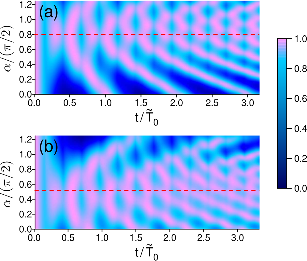
4.4 Pulse-driven charge polarization, currents and magnetic moments in semiconductor quantum rings

Quantum rings (QRs) play a special role in mesoscopic physics bridging classical and quantum-mechanical phenomena [246]. Many intriguing physical effects like the Aharonov-Bohm effect, persistent charge and spin currents, etc. were discovered in these structures [246, 247, 27]. In many cases their physical properties can be captured using single-particle states corresponding to a free angular motion of the electron having an appropriate effective mass and confined to a single radial channel [25, 23, 21, 248, 246, 249, 114, 11] (see Section 3.6.3). Generalization to a multichannel model can be constructed straightforwardly if the radius of the ring is considerably larger than its width and height [115, 11].

Figure 22: Sketch of a QR and the coordinate system. The

z

-axis is directed perpendicular to the plane of the ring.

Let us consider electrons in a thin isolated (without contacts) semiconductor QR with a mean radius $r_{0}$ and width $d$ ( $d\ll r_{0}$ ) at low temperatures (see Fig. 22). It can be made, for example, from GaAs surrounded by AlGaAs having a wider band gap [21] so that up to a certain energy the charge carriers are confined inside the ring. Other material choices are also possible [250]. Its single electron wave functions can be written using cylindrical coordinates $(z,\rho,\varphi)$ as

\psi_{l,m}(z,\rho,\varphi)=Z_{0}(z)R_{l}(\rho)\Phi_{m}(\varphi)\;,

(150)

where $\Phi_{m}(\phi)=\frac{1}{\sqrt{2\pi}}\mbox{e}^{im\varphi}$ is the angular wave function, $R_{l}(\rho)$ denotes the radial wave function; $l=1,2,3\ldots$ and $m=0,\pm 1,\pm 2,\ldots$ are the radial and orbital quantum numbers, respectively. In the $z$ direction the width of the ring is much smaller than $d$ . Therefore, we consider only electrons residing in the lowest $z$ -channel with wave function $Z_{0}(z)$ . If we also assume that $d$ is sufficiently small and the particle number in the ring $N$ is not too large, only single-electron states in the lowest radial subband with $l=1$ are relevant. Such assumptions mean that the thickness and the width of the ring are much smaller than the Fermi wavelength of the confined electrons. This situation is experimentally feasible for semiconductor QRs. Then the single-particle basis is given by $|m\rangle\equiv|\psi_{1,m}\rangle$ so that the free-electron Hamiltonian in the second quantization reads

\hat{H}^{\rm el}_{0}=\sum_{m}\varepsilon_{m}\hat{a}_{m}^{\dagger}\hat{a}_{m}\;,

(151)

where $\hat{a}_{m}^{\dagger}$ and $\hat{a}_{m}$ denote the carrier creation and annihilation operators, respectively. The single-particle energies $\varepsilon_{m}$ are given by Eq. (52). The Hamiltonian of the interaction with a time-dependent external light field, which is polarized in the plane of the QR, is given by

\begin{split}\hat{V}=&-\frac{1}{2}eE_{x}(t)r_{0}\sum_{m}(\hat{a}_{m}^{\dagger}\hat{a}_{m-1}+\hat{a}_{m}^{\dagger}\hat{a}_{m-1})\\ &-\frac{1}{2i}eE_{y}(t)r_{0}\sum_{m}(\hat{a}_{m}^{\dagger}\hat{a}_{m-1}-\hat{a}_{m}^{\dagger}\hat{a}_{m+1}),\end{split}

(152)

where $E_{x}(t)=E_{0x}f_{x}(t)$ and $E_{y}(t)=E_{0y}f_{y}(t)$ are the electric field components. Here $E_{0x}$ , $E_{0y}$ and $f_{x}(t),f_{y}(t)$ denote the corresponding amplitudes and temporal profiles of the ultrashort pulses driving the electron dynamics in the QR, respectively. In the case of semiconductor QRs the relaxation time scales may become comparable with the characteristic system time $\tau_{{}_{\mathrm{F}}}$ (see Section 3.6.3). To account for relaxation one should resort to the density matrix formalism [251, 252, 253]. The density operator components are expressed as $\hat{\rho}_{mm^{\prime}}(t)=\hat{a}_{m}^{{\dagger}}(t)\hat{a}_{m^{\prime}}(t)$ . Taking the expectation value of it with respect to the initial state of the system gives the density matrix components $\rho_{mm^{\prime}}(t)=\langle\hat{\rho}_{mm^{\prime}}(t)\rangle$ . The density matrix provides full information on single-particle evolution.

4.4.1 Relaxation and dephasing in driven quantum rings

Before we start with the description of the system dynamics induced by short broadband pulses, it is important to discuss here the relevant relaxation processes to determine the corresponding relaxation time scales. We consider the semiconductor QR to be free from impurities. Redistribution of the excitation in the system due to the electron-electron collisions is limited by the Pauli blocking and the energy conservation [254]. For typical semiconductor QRs optical phonon energies are much larger than the interlevel energy distance in the neighborhood of the Fermi level. Therefore the main relaxation channels of the excited electronic system of the QR should be governed by the interactions with photon and acoustic phonon fields. Specifically, emission of coherent radiation, spontaneous emission of photons, emission of coherent phonon waves, and scattering by incoherent phonons may play an essential role for the relaxation. In case of semiconductor QRs, these processes were considered in Refs. [117, 118] and are described in Appendices A and B. One can see that the scattering by incoherent phonons determines the largest contribution. At low temperatures the corresponding decay rates may vary from microseconds to picoseconds depending on the temperature and QR parameters (cf. Fig. 47 in Appendix B).

4.4.2 Charge polarization dynamics

The most evident way to induce a field-free charge polarization in a semiconductor QR is to apply appropriate ultrashort HCPs. As far as such pulses deliver momentum kicks to the electronic system of the ring, it is clear that after some time delay the charge distribution of the QR becomes polarized. This, in essence classical, effect was firstly theoretically demonstrated in Ref. [114] for a single-channel semiconductor QR. The model was generalized to the case of a narrow multichannel ring in Ref. [115].

Let us consider the field-free polarization dynamics generated by an applied HCP in more details. The charge polarization of the QR is characterized by its dipole moment that is given by

\boldsymbol{\mu}=\textrm{Tr}[e\mathbf{r}\hat{\rho}]\;,

(153)

where $e$ is the electron charge. The components of $\boldsymbol{\mu}$ can be expressed via near-diagonal density matrix elements as

	$\displaystyle\mu_{x}$	$\displaystyle=$	$\displaystyle er_{0}\sum_{m}\mbox{Re}[\rho_{m,m-1}],$		(154)
	$\displaystyle\mu_{y}$	$\displaystyle=$	$\displaystyle er_{0}\sum_{m}\mbox{Im}[\rho_{m,m-1}]\;.$		(155)

Thus, to access the charge polarization of the QR, one can solve numerically the equation of motion for the single-particle density matrix. Its dynamics is governed by the Hamiltonians (151) and (152) with an appropriate relaxation contribution, as discussed above. The result has to be substituted into Eqs. (154) and (155).

As it was discussed in Section 3.6.3, the IA provides a good description of the excitation process if the parameters of the applied HCP and of the QR are selected properly. In this approximation, selecting the $x$ -axis being parallel to the polarization direction of the applied HCP and using Eq. (22), where the evolution operator is given by Eq. (61) with Eq. (60), leads to [117, 116]

\begin{split}\rho_{m_{1},m_{2}}\!(t)=&\Theta(t){\rm e}^{\frac{i}{\hslash}(\varepsilon_{m_{1}}-\varepsilon_{m_{2}})t}\sum_{mm^{\prime}}C_{m_{2},m}^{*}C_{m_{1},m^{\prime}}\rho_{m^{\prime}\!,m}^{0}(0)\;\\ &+\Theta(-t)\rho_{m^{\prime}\!,m}^{0}(t)\;.\end{split}

(156)

Here the origin of the time axis was selected to coincide with the HCP parameter $t_{1}$ and $\rho_{m^{\prime}\!,m}^{0}(t)$ describes the evolution of the density matrix of the unperturbed QR. $\Theta(t)$ denotes the Heaviside step function. The coefficients $C_{m_{1},m}$ are determined by $C_{m_{1},m}\equiv\langle m|{\rm e}^{i\alpha\cos\phi}|m_{1}\rangle=i^{m_{1}-m}J_{m_{1}-m}(\alpha)$ , where $J_{l}(x)$ is the Bessel function and the parameter $\alpha$ characterizes the strength of the HCP, as it is described in Section 3.6.3. Notice that Eq. (156) does not take account of the relaxation processes and can be therefore used only for sufficiently short times after the excitation. When calculating the induced charge polarization dynamics, we can introduce the corresponding relaxation time via the inverse of the effective decay rate $\tau_{\rm rel}=1/\gamma_{\rm eff}$ of the charge dipole moment of the QR, as it is described in details in Appendix B. Then, assuming that the unperturbed QR has been in an equilibrium state with the density matrix $\rho_{m^{\prime}\!,m}^{0}=f_{m}^{0}\delta_{m^{\prime}\!,m}$ , where $f^{0}_{m}\equiv f^{0}(\varepsilon_{m})$ is the Fermi-Dirac distribution function determined by the temperature and number of the electrons in the QR, and inserting Eq. (156) into Eqs. (154) and (155) gives [116]

\mu_{x}(t)=\Theta(t)er_{0}\alpha h_{1}(t)\sin\!\left(\frac{2\pi t}{t_{p}}\right)e^{-t/\tau_{\rm rel}}\sum_{m}f_{m}^{0}\cos\!\left(\frac{4\pi t}{t_{p}}m\right)

(157)

and $\mu_{y}(t)=0$ . Here the function $h_{1}(t)$ is defined as

h_{1}(t)=J_{0}\big(\Omega_{1}(t)\big)+J_{2}\big(\Omega_{1}(t)\big)\;,

(158)

where the function $\Omega_{1}(t)$ reads

\Omega_{1}(t)=2\alpha\sin(2\pi t/t_{p})

(159)

with

t_{p}=4\pi m^{\ast}r_{0}^{2}/\hslash\;.

(160)

$m^{\ast}$ is the electron effective mass and $r_{0}$ is the QR radius (see Fig. 22).

Figure 23: Numerically calculated field-free dynamics of the QR dipole moment

\mu

induced by a single HCP is shown for different temperatures: (a)

T=0.1

K, (b)

T=0.5

K, (c)

T=1

K and (d)

T=2

K. The HCP shape is determined by Eq. (27) with

\tau_{\rm d}=3

ps and the kick strength

\alpha=0.2

. Parameters of the QR:

r_{0}=1.35~\mu{\rm m}

d=50~{\rm nm}

and

N=400

. The relaxation due to the scattering by phonons is taken into account in the way described in Appendix B for a n-GaAs QR with

c_{{}_{\rm LA}}=4.79\times 10^{5}~\mbox{cm/s},\ \rho_{\rm s}=5.32~\mbox{g/cm}^{-3},\ |D|=8.6~\mbox{eV},\ \hslash\omega_{{}_{\rm D}}=30~\mbox{meV}

, and

m^{*}=0.067m_{0}

(adapted from Ref. [117]).

The field-free dynamics of the QR dipole moment induced by a single HCP is illustrated in Fig. 23, where the result of a numerical solution, including the relaxation as described in Appendix B, is shown for different temperatures. For the chosen parameters of the simulation, the approximate analytical solution (157) gives practically the same dependence. For all temperatures we observe fast (classical) oscillations of the dipole moment (better resolved in Fig. 6) with a period around [255]

T_{\rm cl}=2\pi\hslash/\big|\partial\varepsilon_{m}/\partial m\big|_{m=m_{{}_{\mathrm{F}}}}\approx\tau_{{}_{\mathrm{F}}}\;,

(161)

where $m_{{}_{\mathrm{F}}}$ is the value of the orbital quantum number close to the Fermi level and $\tau_{{}_{\mathrm{F}}}$ is the ballistic time.

In the case of low temperatures and low excitation strengths only the states nearest to the Fermi level contribute to the dynamics. Thus if the highest occupied state of the QR is fully populated before the HCP is applied, only one oscillation frequency is observed. If this state is only partly populated, then oscillations with two close frequencies corresponding to two possible allowed dipole transitions between the populated (partly populated) states and the next higher laying partly empty (empty) states contribute to the dynamics. Therefore, the long-time behavior exhibits beating (see Fig. 23a). With increasing $T$ more levels are only partly populated initially. Therefore, more transitions to the neighboring states become possible. As a consequence, the dynamics of the dipole moment shows alternating collapse and quantum revivals (see Fig. 23b-d). The revival time is given by [255]

T_{\rm rev}=4\pi\hslash/\big|\partial^{2}\varepsilon_{m}/\partial m^{2}\big|_{m=m_{{}_{\mathrm{F}}}}\;

(162)

that agrees with the calculation results shown in Fig. 23. The observed decay of the peak values of the revivals is governed by relaxation processes.

4.4.3 Switching on and off the charge currents

The generation mechanism of charge currents in semiconductor QRs by means of HCPs was firstly described in Ref. [11]. It is a two-step process (see Fig. 24). In the first step, the application of a HCP to the ring results in transient charge polarization, as described above. In the second step, another HCP applied with an appropriate time delay with respect to the first HCP leads to the emergence of a circular charge current in the QR. In the optimal situation, the second HCP should be polarized in the plane of the QR perpendicular to the first HCP.

In the single-channel model the charge current flowing in the QR $I(t)$ can be expressed via the diagonal density matrix components $\rho_{m\!,m}(t)$ as [116]

I(t)=I_{0}\sum_{m}m\rho_{m\!,m}(t)\;,

(163)

where

I_{0}=e\hslash/(m^{\ast}r_{0}^{2})\;.

(164)

Here $e$ denotes the electron charge, i.e. $I_{0}$ is negative. Then with the help of these equations and Eqs. (156), (154) and (155) one can find that the charge current generated by means of the above-described mechanism is given by

I(t)=\Theta(t-\tau)I_{0}\alpha_{\bot}\frac{\mu(\tau)}{er_{0}}e^{-t/\tau_{\rm rel}^{\rm cur}}\;,

(165)

where $\tau$ is the time moment of the application of the second HCP and $\alpha_{\bot}$ is the corresponding kick strength. $\mu(\tau)$ is the charge dipole moment of the QR at $t=\tau$ . Further, $\tau_{\rm rel}^{\rm cur}$ denotes the current relaxation time, an effective relaxation time connected with the relaxation of the diagonal density matrix components [116]. A similar expression to (165) can be obtained also for a multichannel model [11, 245, 152], where a sum over the different radial channels should be performed additionally. In the limit $d\ll r_{0}$ (see Fig. 22), considered here, the charge current $I$ flowing in the QR is associated with an orbital magnetic dipole moment $M$ via the relation

M=\pi r_{0}^{2}I\;.

(166)

Therefore we may interchangeably discuss the generated current and the generated magnetic moment of the QR.

Dependence of $M$ on the time delay $\tau$ between the two applied HCPs and its decay for two particular choices of $\tau$ are illustrated in Fig. 25. We see that there is an optimal time delay between the pulses around $17$ ps leading to the maximal peak value of the emerging current and magnetic moment. This value of the time delay corresponds to $T_{\rm cl}/4$ such that the charge dipole moment generated by the first HCP achieves its maximum value at the time moment of the application of the second HCP. The time dynamics of the magnetic moment shown in the insets demonstrates the relaxation process, which in Ref. [11] was modeled with the help of a single relaxation time $\tau_{\rm rel}^{\rm cur}$ [cf. Eq. (165)]. One can show that an increase of the QR temperature leads to a decrease of the peak value of the generated magnetic moment [11], whereas a larger particle number leads to a smaller $T_{\rm cl}$ [114] and thus enables shorter optimal delay times.

An additional amount of the charge current produced in a QR, where some charge current is already flowing, is independent of the existing current. It can be again described by Eq. (165) and is proportional to the effective strength of the applied HCP and the charge dipole moment of the QR at the time moment when this pulse arrives. This fact together with the property of the dipole moment dynamics to have collapsed phases (see Fig. 23) can be used to switch off completely the current flowing in the ring at a selected time moment. A possibility to create the charge current in the QR and then to eliminate it after a time delay allows to produce short pulses of magnetic field in the neighborhood of the QR. Then one HCP pair is used to switch on the magnetic moment and the second one, coming with a time delay $\tau_{\rm p-p}$ with respect to the first one, is used to switch it off. For a complete switch off we need to know the current value at the time moment when the second pulse pair is applied during the collapsed phase of the charge dipole moment. Thus an appropriate modeling of the relaxation is required in the time range between the HCP sequences for both the charge dipole moment and the current (see Section 4.4.1).

Figure 26: Magnetization pulses generated in the n-GaAs QR by application of two HCP sequences delayed in respect to each other by

\tau_{\rm p-p}=40

ps in (a),

\tau_{\rm p-p}=120

ps in (b), and

\tau_{\rm p-p}=200

ps in (c). Kick strengths of the first three HCPs are the same and are equal to

0.4

, the last HCP has the kick strength:

\alpha_{\bot}^{\prime}=-0.39

in (a),

\alpha_{\bot}^{\prime}=-0.35

in (b), and

\alpha_{\bot}^{\prime}=-0.32

in (c). Dotted lines show the result in the absence of the eliminating pulse sequence. Parameters of the QR:

r_{0}=0.3~\mu{\rm m}

d=20~{\rm nm}

N=160

, and

T=20

K. Parameters of the phonon-induced relaxation are as in Fig. 23 (adapted from Ref. [117]).

The generation of magnetic pulses and its tunability was demonstrated in Ref. [117] and is illustrated in Fig. 26. The magnetic dipole moment shown in this figure is normalized by $M_{0}=\pi r_{0}^{2}I_{0}$ , where $I_{0}$ is given by Eq. (164). The shape of the HCPs used in the simulations corresponds to Eq. (27) with $\tau_{\rm d}=0.5$ ps. Here the first HCP of the generating pulse pair and the first HCP of the eliminating pulse pair are polarized in the same direction and have kick strengths $\alpha=0.4$ , i.e., initiate an identical dynamics of the charge dipole moment in the QR. The second HCP of the generating pulse pair also has the same kick strength $\alpha_{\bot}=\alpha=0.4$ and is polarized in the perpendicular direction in the plane of the QR, antiparallel to the last HCP (second HCP of the eliminating pulse pair). The kick strength of the last HCP $\alpha^{\prime}_{\bot}$ is attenuated with respect to $\alpha_{\bot}$ , in order to compensate for the current relaxation taking place during the time $\tau_{\rm p-p}$ elapsed between the pulse pairs. Possible durations of the generated magnetic pulses are restricted by the relaxation time scale and extension of the collapsed phase of the charge dipole moment dynamics.

4.4.4 Generation of periodic magnetic pulses

The mechanism of the generation and elimination of the charge current and magnetization in the QR can be adapted for the generation of periodic magnetic pulses [117]. One possibility is to repeat both the generating and eliminating pulse sequences periodically in time (see Fig. 27c). As it was discussed in Section 3.10, as any other observable, the magnetization should demonstrate a periodic dynamics after some equilibration stage following the onset of the periodic driving, due to the dissipation in the QR. The resulting periodic magnetization dynamics is shown in Fig. 27a.

Another possibility is to use only the generating pulse sequences (see Fig. 27d). Each pulse sequence compensates for the ongoing current relaxation during the time $\tau_{\rm p-p}$ . Again, an exact compensation, leading to a periodic magnetization dynamics, is achieved after the preceding equilibration stage. The result is shown in Fig. 27b. If $\tau_{\rm p-p}$ is small enough in comparison with the charge current relaxation time scale, a characteristic sawtooth periodic time dependence of the QR magnetization is observed.

4.4.5 Influence of the magnetic flux on the generated charge polarization and currents

The effect of an external static magnetic flux $\Phi$ on the charge polarization and currents generated by HCPs in QRs was studied in Ref. [116]. In such a case the expression for the single-particle energies $\varepsilon_{m}$ in the free-electron Hamiltonian of a one-dimensional QR (151) changes to

\varepsilon_{m}=\frac{\hslash^{2}}{2m^{\ast}r_{0}^{2}}\left(m+\tilde{\Phi}\right)^{2}\;,

(167)

where

\tilde{\Phi}=\Phi/\Phi_{0}

(168)

is the normalized external static magnetic flux with $\Phi_{0}=-hc/e$ being the flux quantum. Then, assuming that the QR is at the thermal equilibrium at $t<0$ , a single HCP polarized along the $x$ -axis and applied to the QR at the time moment $t=0$ induces the charge dipole moment

\mu_{x}(t)=\Theta(t)er_{0}\alpha h_{1}(t)\sin\!\left(\frac{2\pi t}{t_{p}}\right)e^{-t/\tau_{\rm rel}}\sum_{m}f_{m}^{0}\cos\!\left[\frac{4\pi t}{t_{p}}(m+\tilde{\Phi})\right]

(169)

instead of Eq. (157), which is valid for $\Phi=0$ . From Eqs. (167) and (169) it is clear that $\mu_{x}(t)$ is periodic in $\tilde{\Phi}$ with the period being equal to 1. In the case of zero temperature $T=0$ and $N$ electrons in the QR Eq. (169) leads to [116]

\mu_{x}(t)=\Theta(t)er_{0}\alpha h_{1}(t)s(t)e^{-t/\tau_{\rm rel}},

(170)

where

$\displaystyle s(t)\!=$	$\displaystyle 2\cos\!\left[\frac{4\pi t}{t_{p}}\left(\left\|\tilde{\Phi}\right\|\!-\!\frac{1}{2}\right)\right]\sin\!\left[\frac{N\pi t}{t_{p}}\right],\hskip 2.84544pt$	$\displaystyle N\!=0\ ({\rm mod}\;4);$	(171)
$\displaystyle s(t)\!=$	$\displaystyle\cos\!\left[\frac{4\pi t}{t_{p}}\tilde{\Phi}\right]\!\sin\!\left[\frac{(N+1)\pi t}{t_{p}}\right]$
	$\displaystyle+\cos\!\left[\frac{4\pi t}{t_{p}}\left(\left\|\tilde{\Phi}\right\|\!-\!\frac{1}{2}\right)\right]\!\sin\!\left[\frac{(N-1)\pi t}{t_{p}}\right],\hskip 2.84544pt$	$\displaystyle N\!=1\ ({\rm mod}\;4);$	(172)
$\displaystyle s(t)\!=$	$\displaystyle 2\cos\!\left[\frac{4\pi t}{t_{p}}\tilde{\Phi}\right]\sin\!\left[\frac{N\pi t}{t_{p}}\right],\hskip 2.84544pt$	$\displaystyle N\!=2\ ({\rm mod}\;4);$	(173)
$\displaystyle s(t)\!=$	$\displaystyle\cos\!\left[\frac{4\pi t}{t_{p}}\left(\left\|\tilde{\Phi}\right\|\!-\!\frac{1}{2}\right)\right]\!\sin\!\left[\frac{(N+1)\pi t}{t_{p}}\right]$
	$\displaystyle+\cos\!\left[\frac{4\pi t}{t_{p}}\tilde{\Phi}\right]\!\sin\!\left[\frac{(N-1)\pi t}{t_{p}}\right],\hskip 2.84544pt$	$\displaystyle N\!=3\ ({\rm mod}\;4);$	(174)

for $\tilde{\Phi}\in[-1/2,1/2]$ . If $\tilde{\Phi}$ is outside of this range when $s(t;\tilde{\Phi})$ should be determined from the periodicity condition $s(t;\tilde{\Phi}+1)$ = $s(t;\tilde{\Phi})$ . In the absence of the magnetic flux Eqs. (170)–(174) simplify to the result obtained in Ref. [114].

Variations of the dipole moment dynamics when sweeping the magnetic flux are illustrated in Fig. 28 for different values of the HCP kick strength $\alpha$ . In the case of small $\alpha$ we observe a beating behavior. The beating period can be tuned by varying the value of the magnetic flux or the electron number from $t_{p}/2$ to infinity. Higher values of $\alpha$ lead to more complicated time patterns of the dipole moment dynamics, determined by the higher anharmonicity of the function $h_{1}(t)$ in this case. Very high kick strengths give rise to collapses and revivals, due to the large number of states affected by the excitation.

Figure 28: Dynamics of the charge dipole moment

\mu(t)

generated in the QR by a single HCP, calculated from Eq. (170) for various values of the magnetic flux

\Phi

and HCP kick strength

\alpha

t_{p}

is given by Eq. (160). We assume

N=100

T=0

K, and

\tau_{\rm rel}\gg t_{p}

(adapted from Ref. [116]).

In the presence of the static magnetic flux the charge current flowing in the QR is given by

I(t)=I_{0}\sum_{m}(m+\tilde{\Phi})\rho_{m\!,m}(t)\;

(175)

as compared to Eq. (163). Then the current generation mechanism described in Section 4.4.3 leads to the following expression for the total charge current

I(t)=I_{\rm pers}+I_{\rm dyn}(t),

(176)

where

I_{\rm pers}=I_{0}\sum_{m}\left(m+\tilde{\Phi}\right)f_{m}^{0}

(177)

is a static (persistent current) component induced by the magnetic flux [256, 257, 21, 24], which was explicitly calculated in Ref. [258], and $I_{\rm dyn}(t)$ is a dynamical component, which is given by Eq. (165). The static component is determined by the equilibrium distribution function $f_{m}^{0}$ and the magnetic flux $\Phi$ . It remains unaffected by the application of the HCPs. The dynamical component, induced by the HCPs, is a function of the magnetic flux through the corresponding dependence of the dipole moment $\mu(\tau)$ , dictated by Eqs. (169)-(174).

Figure 29 shows the dependence of the charge current flowing in the QR shortly after the application of the generating HCP pair on the time delay $\tau$ between the HCPs and the magnetic flux $\Phi$ . We observe an oscillatory behavior with respect to both $\tau$ and $\Phi$ . An interesting feature observed in Fig. 29 is that the current, which flows in the QR at the thermal equilibrium with nonzero magnetic flux, can be temporarily stopped by an appropriate tuning of the HCP strengths and their mutual delay $\tau$ . The reoccurrence of the persistent current is then determined by the following relaxation of the dynamical component of the current. The total current can be eliminated again if a further HCP pair is applied. A train of HCP, as described in Section 4.4.4, can be used to induce a desired periodic temporal behavior of the current.

4.5 Dynamics of the charge and valley polarization and currents in graphene rings

Graphene QRs represent a particularly interesting type of QRs. One key property of the charge carriers in bulk graphene is their massless quasi-relativistic energy dispersion leading to a number of fascinating phenomena [259, 260, 261, 262, 263, 264]. Another one is that they offer an additional degree of freedom, provided by the valley quantum number $\varkappa=\pm 1$ , which is related to the two nonequivalent positions of the $K$ points in the Brillouin zone. Due to the suppressed intervalley scattering the control of the valley degree of freedom allows for valley-based optoelectronic applications (valleytronics) [265, 266, 267], wherein the generation of pure valley currents is a fundamental goal [268]. Graphene nanostructures driven by ultrashort light pulses may be utilized for the development of novel ultrafast valleytronic devices. The fabrication of graphene QRs was already demonstrated and the Aharonov-Bohm effect was studied in them [27].

Graphene QRs driven by HCPs were studied in Ref. [119]. An approach for describing the single-particle states in graphene QRs was proposed in Ref. [28] (see also Ref. [269]). Let us consider a graphene QR of radius $r_{0}$ and width $d$ (cf. Fig. 22). The ring is threaded by a static magnetic flux $\Phi$ . Properties of the free charge carriers inside the QR are governed by the effective Dirac-Weyl Hamiltonian $H_{0}=v_{{}_{\mathrm{F}}}\boldsymbol{\sigma}\cdot\mathbf{P}$ [260, 261, 262], where $\mathbf{P}=\mathbf{p}-\frac{e}{c}\mathbf{A}_{\rm stat}$ is the momentum operator, modified by the vector potential $\mathbf{A}_{\rm stat}$ of the static magnetic field, and $v_{{}_{\mathrm{F}}}\approx 10^{6}$ m/s is the Fermi velocity in bulk graphene. $\boldsymbol{\sigma}=(\sigma_{x},\sigma_{y})$ , where $\sigma_{x}$ and $\sigma_{y}$ are the corresponding Pauli matrices. They are built on the basis of the pseudospin eigenstates corresponding to the different sublattices of the graphene lattice. The boundary of the ring, causing the quantum confinement of the carriers, is modeled by a potential $\varkappa U(\mathbf{r})\sigma_{z}$ [270, 28, 271], where $U(\mathbf{r})=0$ inside the QR and $U(\mathbf{r})=U_{0}$ outside of it. Thus the Dirac fermions acquire a mass outside of the QR [272, 273]. Such a valley-dependent potential can originate from the interaction of the graphene layer with a nanostructured substrate [274, 275, 272, 273].

The single-particle energies of the charge carriers in the graphene QR are degenerate in spin ( $\pm 1/2$ ) and in the limit $d\ll r_{0}$ (see Fig. 22) can be approximately found as [119]

E_{nm}^{s\varkappa}=s\varepsilon_{n}+s\lambda_{n}\left[m+\tilde{\Phi}^{s\varkappa n}_{\rm eff}\right]^{2}-\frac{s\lambda_{n}}{4\pi^{2}(n+1/2)^{2}}\;,

(178)

with

	$\displaystyle\varepsilon_{n}$	$\displaystyle=$	$\displaystyle(1-\gamma_{0})\frac{\hslash v_{{}_{\mathrm{F}}}}{d}(n+1/2)\;,$		(179)
	$\displaystyle\lambda_{n}$	$\displaystyle=$	$\displaystyle(1+\gamma_{0})\frac{\hslash v_{{}_{\mathrm{F}}}}{d}\left(\frac{d}{r_{0}}\right)^{2}\frac{1}{\pi(2n+1)}\;.$		(180)

Here we have $s=1$ ( $s=-1$ ) for electrons (holes); $n=0,1,2,...$ is the radial quantum number; $m=\pm\frac{1}{2},\pm\frac{3}{2},...$ numerates the angular states. The quantity $\tilde{\Phi}^{s\varkappa n}_{\rm eff}$ in Eq. (178) is given by

\tilde{\Phi}^{s\varkappa n}_{\rm eff}=\tilde{\Phi}-\frac{1}{2}\frac{s\varkappa}{(n+1/2)\pi}\;.

(181)

For fixed $s,\varkappa$ , and $n$ it plays a role of an effective normalized magnetic flux. Notice that with respect to $\tilde{\Phi}$ [as given by Eq. (168)] it contains a valley-dependent shift. The dimensionless factor $\gamma_{0}$ in Eqs. (179) and (180) is determined by

\gamma_{0}=\frac{\hslash v_{{}_{\mathrm{F}}}}{dU_{0}}\;

(182)

and we assumed $\gamma_{0}\ll 1$ . In the case of a graphene QR with a typical width $d=0.1~\mu$ m this implies $U_{0}\gg 7$ meV that is reasonable, e.g., for a hexagonal boron nitride substrate [272, 273].

For brevity, we limit our consideration to the lowest radial channel of the positive energy branch, i.e. $n=0$ and $s=1$ ¹²¹² 12 Experimentally, the filling of quantized energy states in unexcited graphene rings can be controlled by the gate voltage.. Let us find the magnetic dipole moment $\mu(t)$ induced in the graphene QR by the application of a single HCP, polarized along the $x$ -axis, at $t=0$ . Performing analogous steps as in Sections 4.4.2 and 4.4.5, we get

	$\displaystyle\mu(t)$	$\displaystyle=$	$\displaystyle\sum_{\varkappa}\mu_{\varkappa}(t)\;,$		(183)
	$\displaystyle\mu_{\varkappa}(t)$	$\displaystyle=$	$\displaystyle er_{0}\alpha h_{1}(t)\sin\left(\frac{2\pi t}{t_{p}}\right)\sum_{m}f^{\varkappa}_{m}\cos\left[\frac{4\pi t}{t_{p}}(m+\Phi^{\varkappa}_{\rm eff})\right],$		(184)

where $\Phi^{\varkappa}_{\rm eff}\equiv\tilde{\Phi}^{s=1,\varkappa,n=0}_{\rm eff}$ ,

t_{p}=2\pi\frac{\hslash}{\lambda_{0}}\;,

(185)

$h_{1}(t)$ is given by Eq. (158), however with $t_{p}$ from Eq. (185), and $\alpha$ is the HCP kick strength. $f^{\varkappa}_{m}$ is the equilibrium distribution function for the quantum states numbered by $\varkappa$ and $m$ . Here we have neglected the relaxation processes. The dipole moment (183) as well as its valley-resolved parts (184) are periodic in $\tilde{\Phi}$ . The period equals to 1.

Figure 30 shows the dynamics of the generated dipole moment as a function of the magnetic flux for $N=8$ electrons and two different HCP kick strengths. Prior to the excitation the electrons in the QR are in the equilibrium at zero temperature $T=0$ . The complex oscillation structured depending on $t$ and $\tilde{\Phi}$ (Fig. 30a) is a consequence of the interplay between the constituents of Eq. (184). Firstly, the sine and cosine factors oscillate with $t$ and $\tilde{\Phi}$ . Secondly, the discontinuous jumps in the equilibrium distribution $f^{\varkappa}_{m}$ as a function of $\tilde{\Phi}$ occur each time when one of the energy levels [cf. Eq. (178)] crosses the Fermi level [119]. When the HCP kick strength is increased we observe a higher number of oscillation nodes as a function of $t$ (see Fig. 30b), owed to the pronounced anharmonicity of the function $h_{1}(t)$ entering Eq. (184).

Although the effective time-reversal symmetry is broken by the boundary conditions [28] and therefore the energy levels are not invariant under the transformation $\varkappa\rightarrow-\varkappa$ [28], we deduce $\mu_{\varkappa=+1}(t)=\mu_{\varkappa=-1}(t)$ for $\tilde{\Phi}=0$ because of their invariance under the transformation $\varkappa\rightarrow-\varkappa$ , $m\rightarrow-m$ . Only the application of a stationary magnetic flux $\tilde{\Phi}\neq 0$ lifts also this degeneracy between the quantum states, leading to $\mu_{\varkappa=+1}(t)\neq\mu_{\varkappa=-1}(t)$ . This property can be then utilized for the generation of valley-polarized currents in graphene QRs.

The total charge current flowing in the light-driven ring consists of the persistent/static (equilibrium) $I_{\rm pers}$ and dynamical (nonequilibrium) $I_{\rm dyn}(t)$ components [see Eq. (176)], where the persistent charge current is given by [28, 119]

	$\displaystyle I_{\rm pers}$	$\displaystyle=$	$\displaystyle\sum_{\varkappa}I_{\rm pers,\varkappa}\;,$		(186)
	$\displaystyle I_{\rm pers,\varkappa}$	$\displaystyle=$	$\displaystyle I_{0}\sum_{m}f^{\varkappa}_{m}\left(m+\tilde{\Phi}^{\varkappa}_{\rm eff}\right)$		(187)

[cf. Eq. (177)]. Here $I_{\rm pers,\varkappa}$ denotes the contributions from the two different valleys and $I_{0}$ is given by

I_{0}=\frac{1}{\pi^{2}}\frac{ev_{{}_{\mathrm{F}}}d}{r_{0}^{2}}.

(188)

In contrast to the case of single-channel semiconductor QRs [see Eq. (164)], here $I_{0}$ depends not only on the ring radius $r_{0}$ but also on its width $d$ . For a ring with $r_{0}=1~\mu\mbox{m}$ and $d=100~\mbox{nm}$ ( $r_{0}=425~\mbox{nm}$ and $d=150~\mbox{nm}$ ) we have $I_{0}=-0.16~\mbox{nA}$ ( $I_{0}=-1~\mbox{nA}$ ). Utilizing the same mechanism for the current generation as in the case of the semiconductor QRs (see Fig. 24) we find that the dynamical charge current component $I_{\rm dyn}(t)$ is given by Eq. (165), where in the considered case of the graphene QRs $I_{0}$ should be calculated from Eq. (188) and the dipole moment $\mu(\tau)$ at the time moment $t=\tau$ should be determined from Eqs. (183) and (184). As mentioned above, for a nonzero magnetic flux the polarization of the pulse-driven graphene QR becomes valley-dependent. We introduce then the valley current in the ring as $I^{\rm v}=(I_{\varkappa=+1}-I_{\varkappa=-1})/e$ and calculate that its dynamical component induced by the same generating HCP pair as $I_{\rm dyn}(t)$ is given by

I^{\rm v}_{\rm dyn}(t)=\Theta(t-\tau)\frac{I_{0}}{e}\alpha_{\bot}\frac{\mu_{\varkappa=+1}(\tau)-\mu_{\varkappa=-1}(\tau)}{er_{0}}\;.

(189)

Figure 31: The upper panel shows the dependence of the nonequilibrium charge current generated in the graphene QR by application of two mutually perpendicular HCPs, delayed with respect to each other by

\tau

and having kick strengths

\alpha=\alpha_{\bot}=1

. The lower panel shows the nonequilibrium valley current generated by the same pulse sequence. The presented case corresponds to

N=8

and

\tilde{\Phi}=1/\pi

. The arrows indicate time moments when either the generated charge current or the generated valley current vanishes (adapted from Ref. [119]).

An example of the dependencies of the induced nonequilibrium charge and valley currents on the time delay $\tau$ between the HCPs of the generating pulse sequence is presented in Fig. 31. Comparing the upper and the lower panels of this figure, one can see that there are delay times $\tau$ such that either the charge current is present and the valley current vanishes or vice versa. Especially, the second case is of interest because it provides a possibility for a swift generation of pure (nonequilibrium) valley currents in graphene QRs, paving the way towards ultrafast valleytronics.

5 Control of the spin dynamics in semiconductor nanostructures

Light-matter interaction effects in conventional semiconducting nanostructures have been of great interest in view of the diverse applications for photo-electronic devices such as radiation-controlled field-effect transistors, light-emitting diodes, photodiodes, and single-mode optical fiber [276, 277, 278, 279, 280, 281]. The meanwhile well-established field spintronics utilizes in addition the spin degree of freedom exploring its potential for new spin-based devices [282, and references therein]. A variety of materials were under study, including dilute magnetic semiconductors, topological insulators, heterojunctions with ferromagnetic materials, semiconductors, graphene, oxide-based heterostructures and others. Also in many conventional semiconductors, such as GaAs and InSb, the spin degree of freedom is exploitable by means of the strong spin-orbit interaction (SOI). The SOI in bulk semiconductors described by the Luttinger Hamiltonian was predicted to be the key for generating dissipationless quantum spin current at room temperature when applying an electric field in hole-doped semiconductors such as Si, Ge, and GaAs [283]. A similar effect was predicted in a two-dimensional electron gas with Rashba SOI due to a broken inversion symmetry at the interface [284]. The SOI is also central to the spin field-effect transistor (SFET) [285] and spin-interference device [22]. A large conductance modulation effect was predicted in both devices giving impetus to a vast number of studies on the implications and possible applications. Here we discuss semiconductor QRs with SOI and SFET driven by ultrashort electromagnetic pulses. In addition we describe the predicted pulse-induced spatial separation of spin states and coherent control of pure spin currents in double quantum dots. Possible applications are in the areas of the ultrafast spintronics and spin-based quantum computing [286, 287, 288, 282].

5.1 Spin dynamics in semiconductor quantum rings triggered by HCPs

5.1.1 Rashba spin-orbit interaction

The Rashba spin-orbit interaction, SOI, appears in material structures as a consequence of the inversion symmetry breaking. At a heterojunction of two semiconductors this symmetry breaking can be effectively viewed as being induced by a normally oriented electric field due to band bending at the interface. Selecting the $z$ -axis perpendicular to the interface, the Rashba SOI contribution to the Hamiltonian has the form [289, 290, 291]:

H_{\mathrm{R}}=\alpha_{\rm R}[\boldsymbol{\sigma}\times\mathbf{k}]\cdot\mathbf{e}_{z}\;,

(190)

where $\alpha_{\rm R}$ is a parameter reflecting the strength of the SOI, $\mathbf{e}_{z}$ is a unit vector perpendicular to the surface, $\mathbf{k}$ is the wave vector of the charge carrier, and $\boldsymbol{\sigma}$ is the vector of the Pauli matrices. Writing the interface-induced effective electric field as $\mathbf{E}=E_{z}\mathbf{e}_{z}$ , we have $H_{\mathrm{R}}=\frac{\alpha_{\rm R}}{\hslash E_{z}}\boldsymbol{\sigma}\cdot\left[\mathbf{p}\times\mathbf{E}\right],$ where $\mathbf{p}=\hslash\mathbf{k}$ is the carrier momentum ¹³¹³ 13 Please, note that there is a minus sign difference in the definition of the Rashba coefficient in respect to Eq. (1) of Ref. [292] and Eq. (4) of Ref. [285]..

5.1.2 Hamiltonian of a light-driven 1D quantum ring with Rashba effect

Nitta et al. [22] proposed a spin-interference device, namely an Aharonov-Bohm ring with a uniform Rashba SOI, which causes a phase difference between the electron waves with opposite spins traveling in the clockwise and anticlockwise direction. The SOI strength can be controlled by a gate covering the whole ring. A large conductance modulation effect can be expected due to the spin interference. The tunable spin interference in a ring geometry with the SOI thus motivated many studies in the recent past [292, 293, 294, 295, 296, 297, 298, 299, 300, 301, 302, 303, 120, 121, 122]. In presence of an external electromagnetic field and a static magnetic field, directed perpendicular to the plane of the QR ( $\mathbf{B}_{\rm stat}=B_{\rm stat}\mathbf{e}_{z}$ ), the single-particle Hamiltonian in the minimal coupling scheme for an electron confined to the QR reads

H=\frac{\mathbf{\Pi}^{2}}{2m^{*}}+U(\mathbf{r})+e\phi+\frac{\alpha_{\rm R}}{\hslash}(\boldsymbol{\sigma}\times\mathbf{\Pi})_{z}+\frac{1}{2}g\mathbf{\mu}_{B}\boldsymbol{\sigma}\cdot(\mathbf{B}_{\rm stat}+\mathbf{B})\;.

(191)

Here the momentum operator $\mathbf{\Pi}$ can be represented as $\mathbf{\Pi}=\mathbf{P}-\frac{e}{c}\mathbf{A}$ , where $\mathbf{A}$ is the vector potential of the electromagnetic field and $\mathbf{P}=-i\hslash\boldsymbol{\nabla}-\frac{e}{c}\mathbf{A}_{\rm stat}$ ; $-i\hslash\boldsymbol{\nabla}$ is the canonical momentum operator and $\mathbf{A}_{\rm stat}$ is the vector potential of the static magnetic field. $e$ is the electron charge ¹⁴¹⁴ 14 In the case of holes the charge $q=|e|$ should be used in place of the negative electron charge $e$ ., $c$ is the speed of light, $m^{*}$ is the electron effective mass and $g$ is its g-factor in the QR. $\phi$ denotes the scalar potential of the electromagnetic field and $\mathbf{B}$ is its magnetic component. $U(\mathbf{r})$ is the confining potential of the QR. The last term in Eq. (191) is the Zeeman term describing the coupling between the electron magnetic moment $-\frac{1}{2}g\mu_{B}{\boldsymbol{\sigma}}$ and the total external magnetic field $\mathbf{B}_{\rm stat}+\mathbf{B}$ .

Upon a gauge transformation, we can recast the Hamiltonian in the form [120]

H^{\prime}=H_{0}+V(t)\;,

(192)

where

	$\displaystyle H_{0}$	$\displaystyle=$	$\displaystyle\frac{\mathbf{P}^{2}}{2m^{*}}+U(\mathbf{r})+\frac{\alpha_{\rm R}}{\hslash}(\boldsymbol{\sigma}\times\mathbf{P})_{z}+\frac{1}{2}g\mathbf{\mu}_{B}\boldsymbol{\sigma}\cdot\mathbf{B}_{\rm stat}\;,$		(193)
	$\displaystyle V(t)$	$\displaystyle=$	$\displaystyle-e\mathbf{r}\cdot\mathbf{E}(t)+\frac{1}{2}g\mathbf{\mu}_{B}\boldsymbol{\sigma}\cdot\mathbf{B}(t)\;.$		(194)

$\mathbf{E}(t)$ and $\mathbf{B}(t)$ are the electric and magnetic fields of the light pulse, respectively. Using polar coordinates and integrating out the radial dependence in the limit $d\ll r_{0}$ (see Fig. 22), we find for $H_{0}$ [292, 293, 294, 297, 300, 302, 120, 121, 122]

H_{0}=\frac{\hslash\omega_{0}}{2}\left[\left(-i\frac{\partial}{\partial\varphi}+\tilde{\Phi}+\frac{\omega_{R}}{2\omega_{0}}\sigma_{r}\right)^{2}-\left(\frac{\omega_{\mathrm{R}}}{2\omega_{0}}\right)^{2}+\frac{\omega_{B}}{\omega_{0}}\sigma_{z}\right].

(195)

$\sigma_{r}=\sigma_{x}\cos\varphi+\sigma_{y}\sin\varphi$ , $\tilde{\Phi}$ is the normalized external static magnetic flux threading the ring (168), $\hslash\omega_{0}=\hslash^{2}/(m^{*}r_{0}^{2})$ , $\hslash\omega_{\mathrm{R}}=2\alpha_{\mathrm{R}}/r_{0}$ , and $\hslash\omega_{B}=g\mu_{B}B$ .

The stationary eigenstates of $H_{0}$ are

\psi_{m}^{S}(\varphi)=\frac{1}{\sqrt{2\pi}}e^{i(m+1/2)\varphi}\nu_{S}(\gamma,\varphi)\;,

(196)

where $\nu_{S}(\gamma,\varphi)=(a_{S}e^{-i\varphi/2},b_{S}e^{i\varphi/2})^{T}$ are spinors in the angle-dependent local frame and T means transposed. The angular quantum number $m\in\mathbb{N}$ determines the eigenvalue $m+1/2$ of the $z$ -component of the total angular momentum. $S=+1\,(S=-1)$ stands for spin up (spin down) in the local frame. The spinor components can be written as $a_{+1}=\cos(\gamma/2),\;b_{+1}=\sin(\gamma/2),\;a_{-1}=-\sin(\gamma/2),$ and $b_{-1}=\cos(\gamma/2),$ where the angle $\gamma=\gamma(\omega_{\mathrm{R}}/\omega_{0},\omega_{B}/\omega_{0})$ gives the direction of the spin quantization axis, as illustrated in Fig. 32. The corresponding energy spectrum of the QR with the SOI reads

E_{m}^{S}=\frac{\hslash\omega_{0}}{2}\left(m+\tilde{\Phi}^{S}_{\rm eff}\right)^{2}-\hslash\omega_{0}\frac{Q_{\mathrm{R}}^{2}}{8}\;,

(197)

where $Q_{\mathrm{R}}=\omega_{\mathrm{R}}/\omega_{0}$ , $Q_{B}=\omega_{B}/\omega_{0}$ . We have introduced an effective spin-dependent normalized magnetic flux

\tilde{\Phi}^{S}_{\rm eff}=\tilde{\Phi}+\frac{1-Sw}{2}

(198)

with

w=\sqrt{1+Q_{\mathrm{R}}^{2}+4\left(Q_{B}^{2}-Q_{B}\right)}\;,

(199)

in analogy to the energy spectrum of the graphene QRs [cf. Eq. (178)]. If the static magnetic field threading the QR is absent in the QR itself, i.e. there is no Zeeman splitting implicating $Q_{B}=0$ , we can write $Q_{\mathrm{R}}=-\tan\gamma$ and $w=1/\cos\gamma$ .

Figure 32: Schematic graph of the geometry, spin configuration and considered electric field polarization directions (indicated by arrows) of the applied HCPs.

5.1.3 Pulse-driven spin-dependent dynamics and THz emission as indicator for spin precession

For clarity let us focus on the time scale on which relaxation processes are not dominant, in which case one may equally use both the density-matrix approach discussed or a wave function formalism to describe the spin and charge dynamic induced by a HCP ¹⁵¹⁵ 15 In many cases spin relaxation proceeds on a much longer time scale than charge relaxation.. Within the IA the action of a single HCP polarized in the $x$ -direction on a single electron in the QR is determined by Eq. (21), where the evolution operator is given by Eq. (61) and the kick strength $\alpha$ is determined by Eq. (60). The part of the interaction determined by the magnetic field component of the HCP in Eq. (194) is marginal. In fact, the consideration of the second term in Eq. (194) within the IA leads to an additional term $-i\beta\sigma_{y}$ in the exponent of the evolution operator, where $\beta=s_{1}\frac{g\mathbf{\mu}_{B}B_{0}\tau_{\rm d}}{2\hslash}$ . $B_{0}$ denotes the amplitude of the magnetic field and the dimensionless factor $s_{1}$ is defined by Eq. (19). For a typical HCP with electric field amplitude 1 kV/cm and duration $\tau_{\rm d}=1$ ps, the numerical factor $\beta$ characterizing the effective strength of the interaction does not exceed $10^{-5}$ ¹⁶¹⁶ 16 In general this component can be indeed very interesting for exploring the magnetic dynamics at high fields, as demonstrated by recent experiments [304, 305].. Assume that the HCP is applied at $t=0$ ¹⁷¹⁷ 17 This means that the origin of the time axis is selected so that we have $t_{1}=0$ (cf. Section 3.2). Let us consider an electron which occupies the eigenstate characterized by the quantum numbers $m_{0}$ and $S_{0}$ before the HCP application. Then its time-dependent wave function is expressible in terms of the QR stationary eigenstates (196) as

\Psi_{m_{0}}^{S_{0}}(\varphi,t)=\sum_{mS}C_{m}^{S}(m_{0},S_{0},t)e^{-iE_{m}^{S}t/\hslash}\psi_{m}^{S}(\varphi)\;,

(200)

where the expansion coefficients are given by

C_{m}^{S}(m_{0},S_{0},t)=\delta_{SS_{0}}\left[\Theta(-t)\delta_{mm_{0}}+\Theta(t)i^{m_{0}-m}J_{m_{0}-m}(\alpha)\right].

(201)

Here $\Theta(t)$ is the Heaviside step function and $J_{n}(x)$ denotes the Bessel function of the order $n$ . The time-dependent energy $E_{m}^{S}(t)=\langle\Psi_{m}^{S}(t)|H|\Psi_{m}^{S}(t)\rangle$ of the electron being in the state (200) is readily inferred as [114, 120]

E_{m}^{S}(t)=E_{m}^{S}+\Theta(t)\frac{\hslash\omega_{0}}{2}\frac{\alpha^{2}}{2}\;,

(202)

where $E_{m}^{S}$ is given by Eq. (197). Thus, effectively each electron attains an additional amount of energy $\frac{\hslash\omega_{0}}{2}\frac{\alpha^{2}}{2}$ from the HCP. This quantity serves also as the upper limit of energy gain, which is valid irrespective of the situation that a very short HCP might contain very high frequency components.

The charge dipole moment $\boldsymbol{\mu}(t)=\mathbf{e}_{x}\mu(t)$ associated with the intraband coherence induced by the HCP is deduced from Eq. (153) which can be represented as [cf. Eqs. (183) and (184)]:

	$\displaystyle\mu(t)$	$\displaystyle=$	$\displaystyle\sum_{S}\mu^{S}(t)\;,$		(203)
	$\displaystyle\mu^{S}(t)$	$\displaystyle=$	$\displaystyle\sum_{m}f^{S}_{m}\mu_{m}^{S}(t)\;,$		(204)

where $\mu^{S}(t)$ is the spin-resolved dipole moment and $f^{S}_{m}$ stands for the equilibrium distribution function. The contribution to the dipole moment $\mu_{m}^{S}(t)=er_{0}\langle\Psi_{m}^{S}(t)|\cos\varphi|\Psi_{m}^{S}(t)\rangle$ from an electron with the initial state $\psi_{m}^{S}(\varphi)$ can be found as

\mu_{m}^{S}(t)=\Theta(t)er_{0}\alpha h_{1}(t)\sin\left(\frac{2\pi t}{t_{p}}\right)\cos\left[\frac{4\pi t}{t_{p}}(m+\tilde{\Phi}^{S}_{\rm eff})\right],

(205)

where $h_{1}(t)$ is determined by Eq. (158) and $t_{p}$ is given by Eq. (160), i.e. $t_{p}=4\pi/\omega_{0}$ .

In Fig. 33, the time dependence of the dipole moment is shown for different spin-orbit angles $\gamma$ and HCP kick strengths $\alpha$ in absence of the static magnetic field ( $Q_{B}=0,\Phi=0$ ), when we have $\mu^{S=+1}(t)=\mu^{S=-1}(t)$ . The QR contains $N=100$ electrons (i.e. $N=0$ mod 4, whereas the value of $N$ modulo 4 characterizes distinct configurations for the occupation of the states in the neighborhood of the Fermi level) being initially in equilibrium at zero temperature. The quick oscillations have period $T_{\rm cl}$ and frequency $\omega_{{}_{\mathrm{F}}}=2\pi/T_{\rm cl}$ , with $T_{\rm cl}$ given by Eq. (161). In the case $N\gg 1$ , which is valid here, we have $T_{\rm cl}=2t_{p}/N$ and $\omega_{\mathrm{F}}=N\omega_{0}/4$ .

Figure 33: Time dependence of the HCP-induced dipole moment

\mu(t)

at different values of

\gamma

and

\alpha

. There are

N=100

electrons in the QR at

T=0

Q_{B}=0

and

\Phi=0

(adapted from Ref. [120]).

At a low excitation strength, the beating is determined by the difference between the frequencies corresponding to the transitions between the involved states near the Fermi level. Therefore, from Eq. (197) it is clear that the SOI strength (quantified by $\gamma$ ) has a dramatic influence on the low frequency modulation of the envelope of the dipole moment and can lead to a variation of the corresponding low frequency in the range from 0 to $\omega_{0}$ . This means that the beating period can be varied from 0 to $t_{p}/2$ . This behavior in dependence on $\gamma$ is observed in Fig. 33. We see that $\gamma$ can be tuned in such a way that the slow envelope oscillations vanish completely. This happens at $\gamma=-60^{\circ}$ . When $|\gamma|$ is increased further the beating appears again. This is insofar important as $\gamma$ can be modified by an external gate voltage offering thus the possibility of engineering the emission spectrum via an applied static electric field and opening a way for testing experimentally these theoretical predictions. On the other hand the THz emission (power) spectrum deduced from Fig. 33 contains evidently components related to $\gamma$ (cf. Fig. 41c). Recalling that the angle $\gamma$ sets the direction of the spin quantization axis (cf. Fig. 32), theoretically, one may pick up the spin precession by monitoring the relevant emission (which can even be changed, e.g., by a gate voltage that effectively changes the Rashba spin-orbit coupling constant) ¹⁸¹⁸ 18 Note, also in this spin-dependent case the emission is solely electric dipolar in character. Contributions from the magnetic dipole emission are marginal..

Inspecting Fig. 33 we note that with increasing $\alpha$ more states around the Fermi level are excited giving rise to higher contributing harmonics (cf. $\alpha=1$ and $\alpha=3$ in Fig. 33). This affects the dipole moment dynamics in two ways. On one hand, the corresponding anharmonicity makes the time structure more sophisticated. On the other hand, at high enough HCP strengths, we observe a periodic appearance of revivals. The period $T_{\rm rev}$ is determined by Eq. (162), so that we infer that $T_{\rm rev}=t_{p}/2$ . The corresponding frequency is equal to $\omega_{0}$ and thus coincides with the maximum beating frequency. From Fig. 33 we see that the amplitude of the revivals is constant if the beating frequency vanishes ( $\gamma=-60^{\circ}$ ) or if it attains its maximum value ( $\gamma=0^{\circ}$ ). In other cases (e.g. for $\gamma=-30^{\circ}$ and $\gamma=-50^{\circ}$ shown in Fig. 33), a low frequency modulation of the amplitude of the revivals is observed.

5.2 Spin dynamics in 1D semiconductor quantum wires triggered by HCPs and single-cycle pulses

The SFET proposed in 1990 [285] triggered extensive research to validate the performance of this device. Two serious difficulties were overcome in the past. The first is the control of the Rashba SOI in a conductive channel which was demonstrated by Nitta et al. in 1997 using an inverted InGaAs/InAlAs quantum well with a top gate [306]. The second more difficult challenge is the spin-polarized injection into the channel with solutions suggested by various groups [307, 308, 309, 310, 311, 312, 313]. Based on these advances Koo et al. constructed an operational SFET [314]. The analysis was based on the model proposed in Ref. [285]. However this was extended to take into account the angular spectrum in the confinement direction [315]. On the theory side, the SOI effect in a 1D or quasi-1D channel was investigated extensively [316, 317, 318, 319, 320, 321, 322, 323, 324]. Here we review how the spin dynamics and transport in the SFET with a 1D channel can be controlled by the application of broadband ultrashort light pulses [124].

We focus on a 1D quantum wire channel and ignore the spin-flip transitions between the first and second subbands (the energy spacing between these subbands is considered to be too large for the activation of the intersubband transitions). The inversion asymmetry of the confining potential results in the Rashba SOI $H_{\mathrm{R}}$ . For a two-dimensional electron gas in the $xy$ -plane we have $H_{\mathrm{R}}=\alpha^{0}_{\mathrm{R}}(\sigma_{x}k_{z}-\sigma_{z}k_{x})$ , where $\alpha^{0}_{\mathrm{R}}=r_{\mathrm{R}}\mathcal{E}_{0}$ is the static Rashba SOI coefficient, which is proportional to the perpendicular electric field $\mathcal{E}_{0}$ resulting from the band bending, and $r_{\mathrm{R}}$ is a material-specific prefactor [325, 326, 327, 328, 329, 291]. Under equilibrium conditions, spin transport in such a device was investigated extensively [285, 291]; in brief, one chooses the $z$ -axis as the spin quantization axis (Fig. 34) and $x$ for the quantum wire direction, so that $H_{\mathrm{R}}=-\alpha^{0}_{\mathrm{R}}\sigma_{z}k=-\mu_{\mathrm{B}}\sigma_{z}\tilde{B}_{z}$ , where $\mu_{\mathrm{B}}$ is the Bohr magneton, $\tilde{B}_{z}=\alpha^{0}_{\mathrm{R}}k/\mu_{\mathrm{B}}$ is an effective magnetic field along $z$ and $k\equiv k_{x}$ . Usually, one should distinguish two situations: spins are injected from the ferromagnetic leads are aligned (a) parallel to the $z$ -axis and (b) aligned parallel to the $x$ - or $y$ -axis. In the case (a), spins do not precess under the effective magnetic field but feel a spin-dependent potential shift. This results in the splitting $2\alpha^{0}_{\mathrm{R}}k$ between the energies of the injected spins oriented in the $-z$ (down) and $z$ (up) directions. When electrons with spins in the down and up states and the same energy pass through the length $L$ , they acquire an accumulated phase difference

\Delta\theta_{0}=(k_{\downarrow}-k_{\uparrow})L=k_{\mathrm{so}}L\;,

(206)

where $k_{\mathrm{so}}$ is given by

k_{\mathrm{so}}=\frac{2m^{*}\alpha^{0}_{\mathrm{R}}}{\hslash^{2}}\;.

(207)

The eigenenergies and the stationary eigenstates are approximately given by

E_{kS}^{0}=\frac{\hslash^{2}k^{2}}{2m^{*}}-S\alpha_{\mathrm{R}}^{0}k

(208)

and

\psi_{k}^{S}(x)=\frac{1}{\sqrt{L}}e^{ikx}\nu_{S}\;,

(209)

respectively, where $\nu_{S}$ ( $S=\pm 1$ ) denotes the spin states and $m^{*}$ is the effective mass.

Considering the spins to be injected aligned along the $x$ - or $y$ -directions, they precess around $\tilde{\mathbf{B}}_{z}$ . In the Heisenberg picture, the spin operators vary with time as

\dot{\sigma}_{x(y)}(t)=\pm\omega_{k}\sigma_{y(x)}(t)\;,

where

\omega_{k}=\frac{2\alpha^{0}_{\mathrm{R}}k}{\hslash}\;,

(210)

is the precession frequency. It was used that close to the Fermi level we have $k\gg k_{\mathrm{so}}\;$ , i.e. the Fermi energy $E_{\mathrm{F}}$ is much larger than the corresponding spin splitting $2\alpha^{0}_{\mathrm{R}}k$ . The solution of the differential equation above reads

\sigma_{\pm}(t)\equiv\sigma_{x}(t)\pm i\sigma_{y}(t)=\sigma_{\pm}(0)e^{\mp i\omega_{k}t}\;.

Let us specify the initial orientation, say $\sigma_{y}(0)=0$ , then

\sigma_{x}(t)=\sigma_{x}(0)\cos(\omega_{k}t)\mbox{\ \ and\ \ }\sigma_{y}(t)=-\sigma_{x}(0)\sin(\omega_{k}t)\;.

A spin aligned initially along the $x$ -direction rotates clockwise with the angular frequency $\omega_{k}$ . The accumulated angle through the length $L$ amounts to $\Delta\theta_{0}=\frac{2m^{*}\alpha^{0}_{\mathrm{R}}L}{\hslash^{2}}$ , which is exactly equal to the phase shift for the injected spins with the alignment along $z$ .

5.2.1 First dynamic case

Having outlined the equilibrium case, we consider the quantum wire driven by a linearly polarized electromagnetic pulse with the vector potential $\mathbf{A}=\mathbf{e}_{x}A(t)$ . The polarization vector $\mathbf{e}_{x}$ is oriented along the $x$ -direction. We may employ the Coulomb (radiation, velocity) gauge [74, 70] and make use of the dipole approximation. Thus,

\mathbf{E}(t)=-\frac{1}{c}\frac{\partial A(t)}{\partial t}\mathbf{e}_{x}=E_{0}f(t)\mathbf{e}_{x}\;,

(211)

where $E_{0}$ is the peak amplitude of the electric field $E(t)$ and $f(t)$ describes its temporal profile. The single-particle Hamiltonian describing the 1D motion of the electron and its spin dynamics reads [124]

H=\frac{\Pi^{2}}{2m^{*}}-\frac{\alpha^{0}_{\mathrm{R}}}{\hslash}\sigma_{z}\Pi,

(212)

where $\Pi=-i\hslash\frac{\mathrm{d}}{\mathrm{d}x}-\frac{e}{c}A$ . In the Heisenberg picture, it is straightforward to calculate the time-dependent energy expectation value $E_{k_{0}S_{0}}(t)=\langle\psi_{k_{0}}^{S_{0}}|U^{\dagger}(t,0)HU(t,0)|\psi_{k_{0}}^{S_{0}}\rangle$ of an electron being initially in the eigenstate $|\psi_{k_{0}}^{S_{0}}\rangle$ . Here the stationary states $|\psi_{k_{0}}^{S_{0}}\rangle$ are determined by Eq. (209). The evolution operator $U(t,0)$ commutes with $H$ and we get

E_{k_{0}S_{0}}(t)=\frac{1}{2m^{*}}\left[\left(\hslash k_{0}-\frac{e}{c}A(t)-S_{0}\frac{\hslash k_{\mathrm{so}}}{2}\right)^{2}-\frac{\hslash^{2}k^{2}_{\mathrm{so}}}{4}\right],

(213)

where $k_{\mathrm{so}}$ is given by Eq. (207) and $A(t)$ is selected such that it vanishes before the pulse application. Using Eq. (211) we can see from Eq. (213) that after the light pulse is gone the electron energy ${E_{k_{0}S_{0}}(t=\infty)}$ equals to an eigenenergy $E^{0}_{kS_{0}}$ of the unperturbed system, determined by Eq. (208). This eigenenergy corresponds to the state with the same spin $S_{0}$ but with a shifted wave vector

k=k_{0}+\frac{\Delta p}{\hslash}\;,

(214)

where the transferred momentum $\Delta p=-\frac{e}{c}A(t=\infty)$ is given by Eq. (40).

This result can be also obtained if we transform the Hamiltonian (212) into the length gauge [74, 70], like in Section 5.1.2 and Ref. [120], leading to $H^{\prime}=H_{0}+V(t)$ with

H_{0}=\frac{p^{2}}{2m^{*}}-\frac{\alpha^{0}_{\mathrm{R}}}{\hslash}\sigma_{z}p\;

(215)

and

V(t)=-exE(t)\;,

(216)

where $p=-i\hslash\frac{\mathrm{d}}{\mathrm{d}x}$ . Then we use Eq. (21) and proceed like in Section 3.6.1 taking now into account also the spin-dependent part of $H_{0}$ present in Eq. (215). In this way we get that the operator entering the matching condition (21) for the wave functions before and after the pulse is determined by Eq. (39), where $\Delta p$ is given by Eq. (40), $\Delta x$ is given by (41) and $\Delta\phi$ is given by

\Delta\phi=\Delta\phi_{0}-\frac{1}{2}k_{\mathrm{so}}\Delta x\sigma_{z}\;,

(217)

with $\Delta\phi_{0}=s^{\prime}_{3}e^{2}E_{0}^{2}\tau_{\rm d}^{3}/(4m^{*}\hslash)$ , in place of Eq. (42). Thus by this method we see that each electron may get not only a momentum boost $\Delta p$ but also a coordinate shift $\Delta x$ and a spin-dependent phase shift $\propto\Delta x$ from the applied pulse. The spin-independent phase shift, given by the first term on the rhs of Eq. (217), has no physical effect and can be dropped from the present consideration. As it is discussed in Section 3.6.1, depending on the pulse shape we can select the time moment for the matching of the wave functions such that either $\Delta x$ or $\Delta p$ vanish; e.g., for a HCP pulse $\Delta p\neq 0$ and $\Delta x=0$ , whereas for a single-cycle pulse $\Delta p=0$ and $\Delta x\neq 0$ . It is interesting that in any case the accumulated phase difference between the spin-up and spin-down electrons, Eq. (206), remains unchanged by the pulse action. Indeed, the difference $k_{\downarrow}-k_{\uparrow}$ is unaffected by the momentum shift $\Delta p$ experienced by all electrons, and the change in the accumulated phase shift due to the coordinate shift $-k_{\mathrm{so}}\Delta x$ , induced by the pulse, is exactly compensated by the phase difference gained directly from the pulse $k_{\mathrm{so}}\Delta x$ .

Let us consider a particular example of a SFET built on the basis of the GaSb/InAs/GaSb heterostructure [330] with the electron effective mass $m^{*}=0.055m_{0}$ , where $m_{0}$ is the free electron mass. Assuming that the system is driven by single-cycle pulses described in Section 3.3 with the pulse shape parameter $s_{2}=\sqrt{\pi}/2$ and duration $\tau_{\rm d}=50$ fs, such a pulse with a relatively small amplitude of $E_{0}=2$ keV/cm induces a coordinate shift $\Delta x\approx 140$ nm, which is on the order of a typical device length. Thus the operation time can be reduced down to the pulse duration of 50 fs.

Summarizing we conclude that whereas the phase difference $\Delta\theta_{0}$ is maintained as for the static case, the ultrafast momentum boost or coordinate shift experienced by all the electrons can be used to speed up the device operation. This fact is promising for the realization of an ultrafast SFET.

5.2.2 Second dynamic case

Let us consider the case when the electric field polarization direction coincides with the $y$ -axis (see Fig. 34). This electric field $\mathbf{e}_{y}E(t)=\mathbf{e}_{y}E_{0}f(t)$ induces an additional time-dependent SOI [325, 326, 327, 328, 329]. The single-particle Hamiltonian in the length gauge can be written as $H=H_{0}+V(t)$ with $H_{0}$ given by Eq. (215) and

V(t)=-\frac{\alpha^{\mathrm{ind}}_{\mathrm{R}}(t)}{\hslash}\sigma_{z}p\;.

(218)

The time-dependent pulse-induced Rashba SOI coefficient $\alpha^{\mathrm{ind}}_{\mathrm{R}}(t)$ is given by

\alpha^{\mathrm{ind}}_{\mathrm{R}}(t)=r_{\mathrm{R}}E(t)\;.

(219)

From Eq. (16) we obtain for the operator $\mathcal{U}(t_{1})$ describing the action of the pulse on the electrons in the wire

\mathcal{U}(t_{1})=\exp\left(\frac{i}{\hslash}\Delta x_{\mathrm{R}}p\sigma_{z}\right),

(220)

where

\Delta x_{\mathrm{R}}=\frac{s_{1}r_{\mathrm{R}}E_{0}\tau_{\mathrm{d}}}{\hslash}\;.

(221)

Here $\tau_{\mathrm{d}}$ is the pulse duration and the pulse shape parameter $s_{1}$ is determined by Eq. (19). Because $[V(t),H_{0}]$ vanishes, there are no other terms in the exponent of Eq. (220). Inserted into Eq. (21), it provides an exact solution for the electron wave function after the pulse.

In the case of injected electrons with spins aligned parallel to the $z$ -axis, we see from Eq. (220) that the pulse induces a spin-dependent coordinate shift. The spin-down electrons are shifted by $-\Delta x_{\mathrm{R}}$ whereas the spin-up electrons experience a coordinate shift $\Delta x_{\mathrm{R}}$ . In effect, the accumulated phase difference between the spin-down and spin-up electrons with the same energy while traversing the conducting channel is

\Delta\theta=\Delta\theta_{0}+\theta_{\mathrm{p}}\;,

(222)

where $\Delta\theta_{0}$ is given by Eq. (206) and the additional phase difference $\theta_{\mathrm{p}}$ induced by the pulse amounts to

\theta_{\mathrm{p}}=(k_{\downarrow}+k_{\uparrow})\Delta x_{\mathrm{R}}\;.

(223)

Using Eqs. (210) and (221), for the electrons in the neighborhood of the Fermi level with $k\gg k_{\mathrm{so}}$ we infer

\theta_{\mathrm{p}}=\omega_{k}\tau_{\rm d}\frac{s_{1}E_{0}}{\mathcal{E}_{0}}\;,

(224)

where $\omega_{k}$ is given by Eq. (210). For the estimation of the effectiveness of the optical control of the SFET, we analyze the ratio between the pulse-induced and stationary accumulated phase shifts. Using Eq. (207) and (210) in Eqs. (206) and (224) we can write

\frac{\theta_{\mathrm{p}}}{\Delta\theta_{0}}=\frac{2k\Delta x_{\mathrm{R}}}{k_{\mathrm{so}}L}=\frac{v_{\mathrm{F}}\tau_{\rm d}}{L}\frac{s_{1}E_{0}}{\mathcal{E}_{0}}\;,

(225)

where $v_{\mathrm{F}}=\hslash k/m^{*}$ is the electron velocity at the Fermi level. In order to keep the electrons inside the conductive channel upon the pulse application, the condition $\Delta x_{\mathrm{R}}\ll L$ must be fulfilled that limits the pulse strength. Nevertheless, $\theta_{\mathrm{p}}/\Delta\theta_{0}$ can be large if the smallness of $\Delta x_{\mathrm{R}}/L$ is overcompensated by the largeness of $k/k_{\mathrm{so}}$ .

Considering the case of the electron injection with spins aligned along the $x$ or $y$ directions, with the help of Eq. (220) and the same assumptions as above, we find for the spin operators ${\sigma}_{\pm}(t)$ at a time moment $t$ after the pulse

\sigma_{\pm}(t)=\sigma_{\pm}(0)e^{\mp i\omega_{k}t}e^{\mp i\theta_{\mathrm{p}}}.

(226)

The pulse induces a clockwise rotation of the spin by the angle $\theta_{\mathrm{p}}$ , additionally to the rotation angle $\omega_{k}L/v_{\mathrm{F}}$ accumulated over the length of the conductive channel $L$ . Consequently, the total precession angle in the clockwise direction amounts also to $\Delta\theta$ given by Eq. (222).

Let us discuss again a SFET built on the basis of the GaSb/InAs/GaSb heterostructure with $\alpha^{0}_{R}=0.9\times 10^{-9}$ eV cm, the charge density $n=10^{12}$ cm^-2 and $2\alpha^{0}_{R}k=4$ meV at the Fermi level [330]. These values result then in $\omega_{k}\approx 2\pi$ ps^-1 and $v_{\mathrm{F}}=0.4~\mu$ m/ps. Thus in a $L=0.2~\mu$ m long 1D quantum wire there are 20 distributed electrons and the transport time $t_{\mathrm{tr}}$ for the electrons with the Fermi velocity is about 500 fs.

Figure 35: Ratio between the pulse-induced and stationary accumulated phase shifts (precession angles)

\theta_{\mathrm{p}}/\Delta\theta_{0}

in dependence on the HCP duration

\tau_{\mathrm{d}}

and the normalized HCP amplitude

s_{1}E_{0}/\mathcal{E}_{0}

, calculated from Eq. (225). Parameters of the heterostructure and driving HCP are given in the text.

Considering the pulse durations $\tau_{\rm d}$ below 100 fs we have $\tau_{\rm d}\ll t_{\mathrm{tr}}$ and $v_{\mathrm{F}}\tau_{\rm d}<40$ nm, i.e. the factor $v_{\mathrm{F}}\tau_{\rm d}/L$ in Eq. (225) is less than 0.2. HCPs with such durations can be generated with amplitudes $E_{0}$ up to several hundreds of kV/cm. The static fields $\mathcal{E}_{0}$ are typically of the order of several kV/cm [291]. Therefore, taking into account that the HCP pulse shape parameter $s_{1}$ is about one, the factor $s_{1}E_{0}/\mathcal{E}_{0}$ in Eq. (225) can be tuned as high as 100 (without inducing intersubband transitions), so that the ratio $\theta_{\mathrm{p}}/\Delta\theta_{0}$ , calculated after Eq. (225), can be significantly larger than 1. The spin-dependent coordinate shift $\Delta x_{\mathrm{R}}$ does not exceed a value on the order of $100$ nm so that the condition $\Delta x_{\mathrm{R}}\ll L$ can be satisfied.

In Fig. 35 we show a contour plot of the ratio $\theta_{\mathrm{p}}/\Delta\theta_{0}$ as a function of the external field parameters. We clearly see that the pulse-induced phase shift (or rotation angle) is comparable to the static one or may even be significantly larger. We conclude that HCPs can control the spin dynamic in a 1D SFET even playing a dominate role [124]. This opens the way to design an optical SFET, where spin can be engineered via appropriate shaping of electromagnetic pulses.

5.3 Ultrafast spin filtering and its maintenance in a double quantum dot

With the help of additional gate contacts the 1D conductive channel of a heterostructure system like the one shown in Fig. 34 can be transformed into a 1D double quantum dot (DQD) system (see Fig. 36). The zero of the $x$ -axis is selected in such a way that the left (right) quantum dot is located in the region $x<0$ ( $x>0$ ). To control the carrier motion we utilize HCPs polarized either along the $x$ -axis ( $x$ -HCPs) or along the $y$ -axis ( $y$ -HCPs), as illustrated in Fig. 36. Like in Section 4.3, the aim of our consideration is the control of the electron dynamics and its spatial localization, depending now on its spin [125].

The system Hamiltonian is given by $H=H_{0}+V(t),$ where $H_{0}$ represents the Hamiltonian of a free electron in the DQD and $V(t)$ is given by Eq. (216) in the case of $x$ -HCPs or by Eq. (218) in the case of $y$ -HCPs. As it was discussed in Section 4.3, for a certain range of the parameters of the DQD and HCPs we can model the electron dynamics using the two-level system approximation (TLSA), which is extended here to include the spin degree of freedom. Within such an approximation the electron wave function can be represented as

|\Psi(t)\rangle=\sum_{i,s}C_{i,s}(t)|i\rangle|\nu_{s}\rangle\;,

(227)

there $|i\rangle$ with $i=1,2$ denotes the stationary spatial states and $|\nu_{s}\rangle$ with $s=\uparrow,\downarrow$ denotes the spin states. The Hamiltonian of the unperturbed system is given by $H_{0}=-\frac{1}{2}\varepsilon\varsigma_{z}$ [cf. Eq. (66)], where $\varepsilon=\hslash\omega_{21}$ is the distance between the two lowest energy levels of the DQD. We reserve the notation $\boldsymbol{\sigma}=(\sigma_{x},\sigma_{y},\sigma_{z})^{T}$ for the vector of the Pauli matrices in the basis of the spinor states $|\nu_{\uparrow}\rangle,|\nu_{\downarrow}\rangle$ , whereas for the vector of the Pauli matrices in the basis of the pseudospinors states $|i\rangle$ we are going to use here the notation $\boldsymbol{\varsigma}=(\varsigma_{x},\varsigma_{y},\varsigma_{z})^{T}$ ¹⁹¹⁹ 19 Notice the difference in the notation in respect to Section 3.7. We need here different notations for the Pauli matrices in the basis of the spinor states and the Pauli matrices in the basis of the pseudospinor states.. The electron interaction with a $x$ -HCP is given by $V_{v}(t)=-vf_{v}(t)\varsigma_{z}$ [cf. Eq. (66)], where $v=eE^{v}_{0}\langle 1|x|2\rangle$ , $E^{v}_{0}$ is the amplitude of the $x$ -HCP and $f_{v}(t)$ describes its temporal profile. We select the phases of the basis functions such that the coordinate matrix element $\langle 1|x|2\rangle=x_{12}$ is real and positive, whereas the momentum matrix element $\langle 1|p|2\rangle=ip_{12}$ is imaginary. The interaction with a $y$ -HCP reads

V_{u}(t)=-uf_{u}(t)\sigma_{z}\varsigma_{y}\;,

(228)

where

u=\frac{r_{\mathrm{R}}E_{0}^{u}p_{12}}{\hslash}\;,

(229)

$E_{0}^{u}$ and $f_{u}(t)$ are the $y$ -HCP amplitude and its temporal profile, respectively.

Like in Section 4.3, we also utilize the impulsive approximation (IA). In effect the action of the $x$ -HCP on the electron can be reduced to the matching condition (21) with $\mathcal{U}(t_{1})=\exp(i\alpha_{v}\varsigma_{x})$ [cf. Eq. (67)]. Here the dimensionless parameter $\alpha_{v}$ characterizing the strength of the $x$ -HCP is given by $\alpha_{v}=s_{1}^{v}a_{v}$ , where $a_{v}$ is determined by Eq. (68) and $s_{1}^{v}$ should be calculated using Eq. (19). Alternatively, $\alpha_{v}$ can be expressed as $\alpha_{v}=\Delta px_{12}/\hslash$ with $\Delta p$ from Eq. (40). The action of the $y$ -HCP is determined by

\mathcal{U}(t_{1})=\exp(i\alpha_{u}\sigma_{z}\varsigma_{x})\;,

(230)

where the dimensionless parameter $\alpha_{u}$ characterizing the effective strength of the $y$ -HCP can be found as

\alpha_{u}=\frac{\Delta x_{R}p_{12}}{\hslash}\;.

(231)

Here $\Delta x_{R}$ should be calculated from Eq. (221) using the parameters of the $y$ -HCP.

In order to characterize the spin-resolved electron dynamics, we introduce the time-dependent spin-resolved probability to find the electron in the left quantum dot

P_{\mathrm{L}s}(t)=\langle\Psi(t)|\nu_{s}\rangle\langle\nu_{s}|\Theta(-x)|\Psi(t)\rangle\;,

(232)

whereas the total probability to find the electron in the left quantum dot reads $P_{\mathrm{L}}(t)=P_{\mathrm{L}\uparrow}(t)+P_{\mathrm{L}\downarrow}(t)$ . Here $\Theta(x)$ denotes the Heaviside step function. The spin polarization vector in the left quantum dot is given by

\boldsymbol{\Lambda}_{\mathrm{L}}(t)=\frac{\langle\Psi(t)|\boldsymbol{\sigma}\Theta(-x)|\Psi(t)\rangle}{P_{\mathrm{L}}(t)}\;.

(233)

In particular, ${\Lambda}_{\mathrm{L},z}(t)=\left[P_{\mathrm{L}\uparrow}(t)-P_{\mathrm{L}\downarrow}(t)\right]\big/P_{\mathrm{L}}(t)$ .

The time evolution of the system strongly depends on the initial condition. Here it is useful to consider two situations: (a) the initial condition, which corresponds to an electron being completely localized in the left well (tunneling initial condition) and a vanishing average spin along the $z$ -axis, i.e. $\langle\sigma_{z}\rangle=0$ , and (b) the initially delocalized state (optical initial condition) with the same spin properties, which belongs to the ground state of the system. In Ref. [112] it was shown that the optical initial condition can be created from the tunneling initial condition with the help of an appropriate $x$ -HCP applied at an appropriate time moment. Of course, no spin-polarization can be created only by $x$ -HCPs because the excitation is not spin-dependent. The spin polarization can emerge if we apply a $y$ -HCP at the time moment just after a state corresponding to the optical initial condition has been produced. In order to maintain the spin polarization, an appropriate periodic train of $x$ -HCPs can be used, in analogy to the maintenance of spin-unpolarized states (see Sections 4.3.1 and 4.3.3).

Figure 37: Time-dependent probabilities to find a spin-up

P_{\mathrm{L}\uparrow}(t)

(red solid line) and to find a spin-down

P_{\mathrm{L}\downarrow}(t)

(blue dashed line) electron in the left dot. Parameters of the excitation by HCPs are given in the text. For the discussed GaAs-based DQD

T_{0}=0.67

ps (adapted from Ref. [125]).

The results of a numerical simulation realizing this scenario are illustrated in Fig. 37 where the dynamics of the spin-resolved localization probability is shown. We start with the system in the state corresponding to the tunneling initial condition (both spin states have the same probability). After a fixed time $0.25T_{0}$ of the free propagation, where $T_{0}=2\pi/\omega_{21}$ , a $x$ -HCP with $\alpha_{v}=\pi/4$ is applied, which transfers the system into the ground state (both spin states have the same probability $P_{\mathrm{L}\uparrow}=P_{\mathrm{L}\downarrow}=0.25$ ). At $t=0.5T_{0}$ we apply a $y$ -HCP with $\alpha_{u}=\pi/4$ and obtain immediately a nearly perfect spin separation, that means the two spin states are localized in different wells: $P_{\mathrm{L}\uparrow}=0.5$ and $P_{\mathrm{L}\downarrow}=0$ . This separation is then maintained by applying a periodic $x$ -HCP train with the effective strength $\alpha_{v}=\pi/2$ , period $T=0.1T_{0}$ and the first HCP centered at $t=0.56T_{0}$ . In result, afterwards we find for the mean values of the probabilities averaged over the time period $2T_{0}$ : $\langle P_{\mathrm{L}\uparrow}\rangle=0.495$ and $\langle P_{\mathrm{L}\uparrow}\rangle=0.005$ , correspondingly. Thus a very good spin separation is stabilized in time. This is also illustrated in Fig. 38a where the dynamics of the components of the spin polarization $\boldsymbol{\Lambda}_{\rm{L}}(t)$ in the left well is shown. Until the time moment of applying the $y$ -HCP at $t=0.5T_{0}$ the spin polarization in the left well is oriented along the $y$ -axis. Just after this time moment the spin polarization turns abruptly into the $z$ -direction. Its orientation oscillates then inside a small solid angle close to the $z$ -axis under the action of the maintaining $x$ -HCP train. The time average (over $2T_{0}$ ) of the $z$ -component of the spin polarization amounts to $0.982$ . The corresponding trajectory of the polarization vector on the unit sphere is shown in Fig. 38b.

For the experimental realization one might consider a GaAs-based DQD, e.g., with parameters as in Ref. [112], giving $T_{0}\approx 0.67$ ps, and $r_{\mathrm{R}}/|e|\approx 4~\mbox{\AA}^{2}$ [326]. Assuming a HCP duration of $40~\rm fs$ , we estimate that the amplitude of the $y$ -HCPs required to observe the predicted dynamics should be on the order of $10^{7}~{\rm V/cm}$ . Such high and short fields are currently available with the help of the modern short pulse generating techniques [53, 54] but may lead to undesirable effects in the semiconductor heterostructure. Materials with higher values of $r_{\mathrm{R}}$ are required. Narrow gap semiconductors, e.g. InSb, would be more promising in this respect because of the much higher values of $r_{\mathrm{R}}$ compared to GaAs [326].

We have discussed how to separate the spin states of electrons in a DQD by application of two delayed HCPs. In this way a nearly perfect spin polarization can be achieved and then maintained for a desired period of time by applying an additional HCP train. Such light-induced spin filtering can be realized on a sub-picosecond time scale that can be of relevance for designing ultrafast spintronic and spin-qubit devices [286, 287, 288, 282].

5.4 Generation and coherent control of pure spin current via THz pulses

Figure 39: The double quantum well structure is considered with the additional feature that in the left well the charge carriers experience a local spin-orbital coupling (red arrow), i.e. a wave packet with a spin up (green arrow) in the right well changes spin orientation when traversing the left well. As discussed in the text, however, starting with a spin-polarized population in the right well [i.e.,

\langle\sigma_{z}\rangle(t=0)=1

], we can apply short pulses stabilizing this state in time, i.e. blocking tunneling. The appropriate pulse sequence is marked (i). No spin dynamics takes place during this time. Allowing for tunneling (time interval between pulse sequences i and ii) and maintaining the charge localization in the left well (pulse sequence ii) initiates the spin dynamics leading to a steady decrease in

\langle\sigma_{z}\rangle

and hence an increase in

\langle\sigma_{y}\rangle

, which means in turn a net pure spin current. The results are averaged over the fast electronic transient oscillations. It is even possible to use the pulse sequence (iii) and stop the spin dynamics within picoseconds. The full lines in the left top panel are results of a full numerical time propagation, whereas the circles are the outcome of an analytical adiabatic decoupling of the electronic and spin dynamics. (Figure is due to Ref. [123]).

We have seen that pulse trains are capable of triggering directed charge currents and spin-polarized currents. A relatively recent development is the generation and utilization of pure spin currents in an open circuit geometry, i.e. a flow of angular momentum without a net charge current [331, 332, 333, 334, 335, 336, 337, 338, 339, 340]. The main focus has been on triggering this current by a temperature gradient in materials that exhibit an exchange spin torque with a non-uniform temperature distribution, or by spin pumping (e.g., via ferromagnetic resonance) in a ferromagnetic/paramagnetic structure, and exploiting the spin-orbital coupling that has to be present in the paramagnet (e.g., platinum). The interest is motivated by potential applications in spintronic devices with low-energy consumption. Another way to avoid the use of magnetic fields or high current-density, spin-polarized current for magnetic switching is to generate the pure spin current by optical means using ultrashort THz pulses [123]. The general idea exploits the different time scales of the charge (generally in the atto- to femtosecond time scale) and spin dynamics (usually in the pico- to nanosecond time scale). Thus, driving the system with a residual spin-orbit coupling by a sequence of ultrashort HCPs of moderate intensity results in a fast pure electronic transient accompanied by a much slower transversal spin dynamics (longitudinal spin dynamics is much higher in energy and requires orders of magnitude higher intensity than discussed here). Therefore in an open circuit geometry, a time average on the time scale of the spin dynamics results in pure spin phenomena. An explicit demonstration was given in Ref. [123] for the generation of a pure spin current by a sequence of THz HCPs of moderate intensity. A typical result is shown in Fig. 39 for the DQD structure which we discussed above with the difference that a SOI is operational in one of the wells, say the left well. Thus, starting with a spin-polarized (green arrow, which also defines the $z$ -direction in Fig. 39) state localized in the right well and driving the charge dynamics by the pulse sequence plotted in the left bottom panel of Fig. 39 results in a well-defined spin rotation once the wave packet is in the left well. The rotation proceeds on a much longer time scale than the tunneling. Hence, we may adiabatically decouple these two types of motions, as shown in Ref. [123]. This yields semi-analytical expressions that agree very well with the full numerical solution, as evident from Fig. 39 endorsing a posteriori the possibility of a dynamic decoupling of charge and spin. Indeed, as demonstrated in Fig. 39, upon averaging over the fast oscillations due to the electronic transient, the pulse sequence leads to a pure spin current. Interestingly this current can even be controlled coherently by applying an appropriate pulse sequence, which is a clear advantage over thermal schemes for generating pure spin currents by utilizing a thermal gradient.

6 Light emission from quantum systems driven by short broadband pulses

How to capture theoretically the radiation emitted from electrons moving along confined trajectories is an old problem, probably first addressed in 1907 by Schott in connection with the question of as how to describe the discrete atomic emission spectra in the framework of the classical electrodynamics [341]. It is clear that the emission spectra encode certain information about the electronic system and also about its dynamics. Thus they provide a possibility for the experimental characterization and control of the system dynamics. This is especially important for ultrafast processes in small quantum systems where a direct observation of this dynamics can be a challenge.

On one hand, in connection with the spectral measurements, ultrashort broadband pulses provide an excellent tool for the characterization of electronic systems on ultrafast time scales, allowing for the separation of the excitation process and the following field-free system dynamics. The generated emission can be detected in the absence of the influence of the driving fields. On the other hand, the electron dynamics, controlled by such electromagnetic pulses, can be monitored via the emission spectra. It is possible to check if the system is in a particular target state or if it follows the prescribed dynamics. Finally, the light emitted from the pulse-driven quantum systems, e.g., nanostructures, might have interesting properties so that it, in its turn, can be used for further application.

Here we review several examples of the stationary spectra of the pulse-driven quantum systems. Then we discuss the time-dependent spectrum and the control of the circular polarization degree by means of broadband, ultrashort pulses.

6.1 Stationary spectra

Firstly, we are going to study the stationary (time-integrated) emission spectra $I_{s}(\omega)$ of the pulse-driven quantum systems. In a non-relativistic case at large distances from the emitting system we have (see Appendix C)

I_{\mathrm{s}}(\omega)\propto\omega^{4}|\mu_{\omega}|^{2}\;,

(234)

where $\boldsymbol{\mu}_{\omega}$ is the Fourier component of the dipole moment. If the spectrum is limited to a some frequency range such that its width $\Delta\omega$ is much smaller than the frequencies $\omega$ inside this range, then it is sufficient to consider just $|\mu_{\omega}|^{2}$ . However, if this condition is not fulfilled, it is important to remember about the additional factor $\omega^{4}$ in Eq. (234) when comparing the calculations with experimentally measured spectra.

6.1.1 Spectra of 1D double quantum wells driven by periodic HCP trains

The emission spectrum of 1D DQWs driven by periodic trains of HCPs was analyzed in Refs. [112, 342]. The dipole moment $\mu(t)$ is connected with the time-dependent probability to find the electron in the left well $P_{\mathrm{L}}(t)$ as

\mu(t)=d_{12}\left[2P_{\mathrm{L}}(t)-1\right],

(235)

where $d_{12}$ is the (real) transition dipole matrix element. Thus the emission spectra can be obtained from the numerically calculated dynamics of $P_{\mathrm{L}}(t)$ , which was discussed in Section 4.3. In Fig. 40 $|\mu_{\omega}|^{2}$ , i.e. $I_{\mathrm{s}}(\omega)/\omega^{4}$ , is presented for a DQW driven by a periodic train of HCPs. Different HCP strengths are selected in Figs. 40a-40c, whereas other simulation parameters are the same as for the full numerical calculations of Fig. 16. In particular, in the considered case the pulse train frequency $\omega_{T}$ , defined by Eq. (80), is much larger than characteristic system frequency $\omega_{21}$ , determined by Eq. (130): $\omega_{21}/\omega_{T}\approx 0.15$ .

Figure 40: Spectra

|\mu_{\omega}|^{2}

from a DQW driven by periodic trains of HCPs with peak electric fields: (a) 150 kV/cm, (b) 168.37 kV/cm, and (c) 84.068 kV/cm. The corresponding values of the parameter

\alpha

, defined by Eq. (138), are

\alpha=0.89\pi

in (a),

\alpha=\pi

in (b), and

\alpha=\pi/2

in (c). Other parameters are as in Fig. (16). The frequency is normalized by

\omega_{T}=2\pi/T

, where

T

is the period of the HCP train (adapted from Ref. [112]).

To comprehend the structure of these spectra, it is worthwhile to consider the Floquet representation (79) of the wave function of the periodically driven electron within the TLSA. Decomposing the Floquet modes into the Fourier series,

|\Phi_{\lambda}(t)\rangle=\sum_{n=-\infty}^{\infty}|b_{\lambda n}\rangle e^{in\omega_{T}t}\;,

(236)

leads to [241, 112]

|\mu_{\omega}|^{2}=4\pi^{2}|i_{1}+i_{2}+i_{3}|^{2}\;,

(237)

where

$\displaystyle i_{1}$	$\displaystyle=$	$\displaystyle\sum_{\lambda=1}^{2}\|C_{\lambda}\|^{2}\sum_{n,n^{\prime}=-\infty}^{\infty}\langle b_{\lambda n}\|x\|b_{\lambda n^{\prime}}\rangle\delta\big((n^{\prime}-n)\omega_{T}-\omega\big)\;,$	(238)
$\displaystyle i_{2}$	$\displaystyle=$	$\displaystyle C_{1}C_{2}^{*}\sum_{n,n^{\prime}=-\infty}^{\infty}\langle b_{2n}\|x\|b_{1n^{\prime}}\rangle\delta\big((n^{\prime}-n)\omega_{T}+(\epsilon_{2}-\epsilon_{1})/\hslash-\omega\big)\;,$	(239)
$\displaystyle i_{3}$	$\displaystyle=$	$\displaystyle C_{2}C_{1}^{*}\sum_{n,n^{\prime}=-\infty}^{\infty}\langle b_{1n}\|x\|b_{2n^{\prime}}\rangle\delta\big((n^{\prime}-n)\omega_{T}+(\epsilon_{1}-\epsilon_{2})/\hslash-\omega\big)\;.$	(240)

Here $\epsilon_{1}$ and $\epsilon_{2}$ are the quasienergies determined by Eq. (137). One can see from these equations that in the general case the spectrum ( $\omega\geq 0$ ) consists of peaks located at (i) $\omega=N\omega_{T}$ , (ii) $\omega=(N+1)\omega_{T}\pm(\epsilon_{2}-\epsilon_{1})/\hslash$ , and (iii) $\omega=(\epsilon_{2}-\epsilon_{1})/\hslash$ . Here $N=0,1,2,\ldots$ . Note that $(\epsilon_{2}-\epsilon_{1})/\hslash$ is positive and does not exceed $\omega_{T}$ (see Fig. 17). The peaks of all these three types can be observed in Fig. 40a.

Assuming $\omega_{21}<\omega_{T}/2$ , the minimum of both $(\epsilon_{2}-\epsilon_{1})/\hslash$ and $\omega_{T}-(\epsilon_{2}-\epsilon_{1})/\hslash$ equals to $\omega_{21}$ . It is achieved when the delocalization condition (143) is fulfilled. In this case HCPs do not influence the dynamics of the electron that is oscillating between the quantum wells. Then only one peak in the spectrum at the frequency $\omega_{21}$ survives. This situation corresponds to Fig. 40b.

Finally, in the case $(\epsilon_{2}-\epsilon_{1})/\hslash=\omega_{T}/2$ the peaks of the types (ii) and (iii) are positioned at half-integers of $\omega_{T}$ . The peak of the type (ii) with the lowest frequency coincides with the peak of the type (iii). Each of the other peaks of the type (ii) coincides with one another peak of the same type. Thus there are two times less peaks per frequency interval than in a general case. This situation corresponds to the condition (145), which is necessary for the suppression of tunneling. If another necessary condition $\omega_{21}/\omega_{T}\ll 1$ is also fulfilled, that is the case here, then choosing an appropriate initial condition we have an electron persistently localized in the left well (cf. Fig. 16a). The corresponding spectrum is displayed in Fig. 40c.

6.1.2 Driven quantum rings as THz emitter

Stationary spectra of semiconductor quantum rings excited by a single HCP were discussed in Ref. [117]. In particular, their temperature dependence was analyzed in connection to the beating, revivals and collapses observed in the polarization dynamics (cf. Section 4.4.2). An example, of the temperature-dependent spectra is shown in Fig. 41a. Figure 41b from Ref. [120] illustrates the dependence of the spectra on the HCP kick strength $\alpha$ . At low temperature and low excitation strengths we observe two peaks. This follows from the properties of the distribution function in the neighborhood of the Fermi level. Here we have the electron number $N=400$ for Fig. 41a and $N=100$ for Figs. 41b, i.e. there is an even number of electrons in each spin channel. Therefore, at zero temperature all levels with angular quantum numbers $|m|<N/4-1$ are occupied, the occupation of the levels with $m=\pm N/4$ equals to 1/2, and the levels with $|m|>N/4$ are empty. As a consequence, at low excitation strengths only the transitions between the states with $|m|=N/4-1$ and $|m|=N/4$ and between the states with $|m|=N/4$ and $|m|=N/4+1$ (whereas $m$ does not change its sign) contribute to the dipole moment dynamics, where we observe the beating in this regime (see Fig. 23), leading to the emission spectrum with the two corresponding peaks. They are located at $\omega=(N/2-1)\omega_{0}/2$ and $\omega=(N/2+1)\omega_{0}/2$ . Increasing the temperature, we increase the number of levels which are only partly occupied. Therefore more transitions are involved in the dynamics, resulting in the interchanging revivals and collapses (cf. Fig. 23), and contribute to the emission spectrum (see Fig. 41a). The same happens when increasing the effective HCP strength $\alpha$ (see Fig. 41b) because more states in the neighborhood of the Fermi level are affected by the excitation. Peaks at $(N/2\pm 3)\omega_{0}/2,(N/2\pm 5)\omega_{0}/2,...$ appear. The corresponding energy range is determined by the energy $\hslash\omega_{0}\alpha^{2}/4$ transferred by the HCP to an electron in the QR [cf. Eq. (202)]. In Fig. 41a we see that the temperature increases not only multiplies the number of peaks but also makes them less pronounced due to the smaller relaxation times (cf. Fig. 47), which determine the spectral broadening. Small relaxation times lead to the smearing out of the peaks so that finally only one broad peak can be distinguished.

Figure 41: (a) Emission spectra

I_{\mathrm{s}}(\omega)

of a semiconductor QR excited by a single HCP for different values of temperature. The spectra are calculated for the charge polarization dynamics shown in Fig. 23. They are offset vertically for clarity. (b) Emission spectra for different values of the HCP kick strengths

\alpha

. No SOI is present in this case. (c) Emission spectra for different SOI strengths, quantified by the angle

\gamma

(see Fig. 32). In (b)

\gamma=0

whereas in (c)

\alpha=0.01

is fixed; in both cases the frequency

\omega

is normalized by

\omega_{0}/2

\omega_{0}=\hslash/(m^{*}r_{0}^{2})

[cf. Eq. (195)], there are

N=100

electrons in the QR at zero temperature [(a) is adapted from Ref. [117], (b) and (c) are adapted from Ref. [120]].

Figure 41c illustrates how the SOI modifies the spectra at zero temperature in the low excitation regime. Enahncing $|\gamma|$ , which characterizes the SOI strength, we observe a blue shift of the lower frequency peak and a red shift of the higher frequency peak, until they merge at $\gamma=-60^{\circ}$ (cf. also the left bottom panel of Fig. 33). A further increase of the SOI strength (not shown in Fig. 41c) leads to the reappearance of the peak splitting and their motion towards the initial positions at $\gamma=0$ .

In Refs. [114, 343] stationary spectra of semiconductor quantum rings excited by a HCP train were studied in the limit case when the period of the train $T$ is much larger than the relaxation time $\tau_{\rm rel}$ . In such a case, one easily finds:

|\mu_{\omega}|^{2}=\big|\mu^{\rm 1HCP}_{\omega}\big|^{2}\left[\frac{\sin(k\pi\omega/\omega_{T})}{\sin(\pi\omega/\omega_{T})}\right]^{2}\;,

(241)

where $\mu^{\rm 1HCP}(t)$ is the time-dependent dipole moment created in the QR by a single HCP.

Figure 42 shows $|\mu_{\omega}|^{2}$ calculated for a train with $k=10$ HCPs. One can observe peaks positioned at multiples of $\omega_{T}=2\pi/T$ . This reflects the behavior of the second factor on the rhs of Eq. (241). The heights of the peaks are modulated by the function $k^{2}\big|\mu^{\rm 1HCP}_{\omega}\big|^{2}$ , representing the amplified spectrum of the QR excited by a single HCP. Using a train of HCPs one can considerably amplify the radiation intensity and, at the same time, via the modulation function retrieve the spectrum generated by a single HCP. Figure 42a corresponds to the low excitation regime ( $\alpha\ll 1$ ) whereas Fig. 42b is calculated for the strong excitation regime. In the latter case the broadening of the modulation function is larger due to the reasons discussed above for the single-pulse excitation.

6.1.3 High-harmonic emission from quantum rings driven by THz broadband pulses

As we could see above, the emission spectrum of HCP-driven QRs is confined to a frequency range around the central frequency $\omega_{{}_{\mathrm{F}}}=N\omega_{0}/4$ , where $\omega_{0}=\hslash/(m^{*}r_{0}^{2})$ . Interestingly, inspired by the rescattering model for high-harmonics generation [344], one may expect a strong modulation of the emission spectra in a range well beyond $\omega_{{}_{\mathrm{F}}}$ due to scattering impurities or engineering a scattering/tunneling potential in the QR. This idea was followed in Ref. [345], where a QR with a localized impurity was considered. Such an impurity can be realized, e.g., by cutting the QR at one place [346] or by fabricating a small part of the ring from a material with a broader band gap. The single-particle Hamiltonian for a free electron (51) is then modified by an additional angular potential $V_{\mathrm{imp}}(\varphi)$ , which for an impurity located at $\varphi=0$ (see Fig. 22) can be modelled as $V_{\mathrm{imp}}(\varphi)=\Omega\delta(\varphi)$ , where the barrier strength $\Omega$ is measured in units of energy times angle interval. For this model a semi-analytical treatment is possible [345].

In case of an excitation by a HCP with the electric field component polarized along the $x$ -axis, the emission spectrum is practically the same as for a ring without the impurity. The reason lies in the symmetry of the problem [345]. The electron density driven by the HCP bounces off the impurity that leads to the generation of the electromagnetic field. However, in the far-field region the field generated by electrons moving towards the impurity in the clockwise direction and then scattered by it is compensated by the field generated by electrons moving in the opposite direction.

Figure 43: Emission spectra of a HCP-driven QR with a localized impurity for different values of the HCP kick strength

\alpha

and impurity barrier strength

\Omega

: (a)

\alpha=0.1

\Omega=0

; (b)

\alpha=0.1

\Omega=0.5

meV rad; (c)

\alpha=0.1

\Omega=10

meV rad; (d)

\alpha=10

\Omega=0

; (e)

\alpha=10

\Omega=0.5

meV rad; (f)

\alpha=10

\Omega=10

meV rad. The calculations are produced assuming the dipole moment relaxation time

\tau_{\rm rel}=1

ns and zero temperature. Other QR parameters:

r_{0}=132~

nm,

m^{*}=0.067m_{0}

and

N=20

, resulting in

\omega_{{}_{\mathrm{F}}}=0.08~

THz (adapted from Ref. [345]).

The situation changes if a HCP with the polarization along the $y$ -axis is used. Here the mirror symmetry of the nonequilibrium electron density in respect to $\varphi=0$ is broken that leads to the generation of coherent light bursts by the scattered electrons. In Fig. 43 the emission spectrum of the driven QR is shown for different HCP kick strengths $\alpha$ and impurity barrier strengths $\Omega$ . In Figs. 43a-c the excitation strength is low ( $\alpha=0.1$ ) and the barrier strength is varied. In the absence of the impurity (Fig. 43a) we observe two peaks in the spectrum, as already discussed above. The increase of the impurity barrier strength leads to a blue shift of the peaks and the appearance of additional peaks both below $\omega_{{}_{\mathrm{F}}}$ and above it (see Figs. 43b,c).

In the case of a strong excitation ( $\alpha=10$ ), illustrated by Figs. 43d-f, we see many peaks already without the impurity because many levels are affected by the excitation [cf. Eq. (202)]. This, together with a relatively small number of electrons ( $N=20$ ) in the QR, is also the reason for the higher frequencies present in the spectrum in respect to the low excitation case. The introduction of the impurity enables transitions not only between neighboring levels but also between distant levels affected by the excitation. Therefore, apart from the blue shift of the spectrum and appearance of additional frequencies in the frequency range of Fig. 43, also much higher frequencies can be observed in the spectrum.

Figure 44: High frequency range of the emission spectra corresponding (a) to Fig. 43e and (b) to Fig. 43f (adapted from Ref. [345]).

In Fig. 44a we can see that for $\Omega=0.5$ meV rad frequencies up to around $28\omega_{{}_{\mathrm{F}}}$ and for $\Omega=10$ meV rad (and also larger impurity barriers [345]) frequencies up to around $35\omega_{{}_{\mathrm{F}}}$ are present in the spectrum. For the parameters of the simulations the latter value corresponds approximately to 3 THz. Therefore, appropriately manufactured arrays of the QR with impurities can be potentially used as sources of coherent THz radiation [345]. As far as the high harmonics are absent for the $x$ -polarized HCPs, the effect could be also utilized for the detection of positions of localized defects in QRs by measuring the emission spectrum while rotating the HCP polarization.

6.2 Time-dependent spectra

Figure 45: Time-dependent spectra of a HCP-driven QR calculated after Eq. (293). The spectra are normalized to

S_{\rm norm}=\frac{e^{2}r_{0}^{2}\omega_{\mathrm{F}}^{3}}{4\pi c^{3}}

. The QR is excited (a) by two mutually perpendicular HCPs with kick strength

\alpha=0.4

and delay

T_{\rm cl}/4

separating them in time and (b) by similar HCP pairs, but with kick strength

\alpha=0.1

, which are repeatedly applied with the period equal to

T_{\rm cl}

(cf. Fig. 27d). The temporal profile of the HCPs used in the simulations is determined by Eq. (27) with

\tau_{\rm d}=0.5

ps and the peak electric field equal to 33.6 V/cm in (a) and 8.4 V/cm in (b). Detector time used in Eq. (291) amounts to

\Delta T=100

ps. Parameters of the QR and phonon-induced relaxation are as in Fig. 26, except for the temperature, which is

4

K in (a) and

10

K in (b) (adapted from Ref. [118]).

In Ref. [118] the time-dependent spectrum (see Appendix C) was studied for HCP-driven QRs. Figure 45a shows the time-dependent spectrum for a QR after the excitation by a sequence of two HCPs, which are polarized in the plane of the QR perpendicular to each other and separated by the time interval $T_{\rm cl}/4$ , where $T_{\rm cl}/4$ is determined by Eq. (161). The spectrum exhibits repeated light bursts, which are centered in frequency at approximately $\omega_{{}_{\mathrm{F}}}$ and have peak values decaying with time due to the relaxation. The bursts correspond to revivals of the charge polarization dynamics [117]. The abrupt radiation switch-on, when the charge polarization is generated by the HCPs, results in a relatively broad spectrum at short times. Figure 45b illustrates that the emission can be effectively stabilized (cf. Section 3.10) if the QR is driven by a periodic train of HCPs so that the time-dependent spectrum reaches a practically stationary state.

6.3 Ultrafast control of the circular polarization degree of the emitted radiation

The driving by HCP pairs used in the numerical calculations of Fig. 45 is such that it creates a rotating dipole moment in the QR. The magnitude of the dipole moment oscillates and decays in time for Fig. 45a whereas it is stabilized for Fig. 45b. Such a dynamics of the dipole moment leads to the circular polarization of the radiation emitted in the direction perpendicular to the QR, similar to the synchrotron radiation [347]. This can be detected by measuring the corresponding time-dependent degree of circular polarization $P_{\mathrm{circ}}^{\bot}(t)$ at any time moment $t$ after the excitation (see Appendix D for an appropriate definition of this quantity). For the frequency range of detection $[0.5\omega_{{}_{\mathrm{F}}},1.5\omega_{{}_{\mathrm{F}}}]$ and detector time $\Delta T=100$ ps, we find $P_{\mathrm{circ}}^{\bot}(t)>0.99$ in the case of the oscillating and decaying magnitude of the induced rotating dipole moment in the QR (corresponding to Fig. 45a) and $P_{\mathrm{circ}}^{\bot}(t)>0.999$ in the case of the stabilized magnitude (corresponding to Fig. 45b). In both cases an ultrafast generation of the circularly polarized light from the QR is realized.

Figure 46: Time-dependent degree of circular polarization characterizing the emission of the HCP-driven QR. The QR is driven by a periodic train of HCPs. There are four HCPs in each period of the train. The first (second) pulse pair in the period consists of two mutually perpendicular HCPs with kick strengths

\alpha_{\|}=0.2,\ \alpha_{\bot}=0.2

(

\alpha_{\|}=0.2,\ \alpha_{\bot}=-0.2

) and delay time

T_{\rm cl}/4

between them (cf. Fig. 27c). Time delay between the HCP pairs amounts to 0.7 ns (which is large in respect to

T_{\rm cl}/4

). Duration of each HCP is

\tau_{\rm d}=3

ps. Detector time is

\Delta T=100

ps. Temperature is

4

K and the other QR and relaxation parameters are as in Fig. 23 (adapted from Ref. [118]).

As it was proposed in Ref. [118], by an appropriate driving by HCPs the degree of circular polarization can be manipulated on ultrafast time scales. For example, we can design a train of HCPs so that each next pair of the HCPs in the train changes the sense of rotation of the QR dipole moment. This leads to the corresponding sign changes of $P_{\mathrm{circ}}^{\bot}(t)$ , as demonstrated in Fig. 46. Thus the photons are emitted in portions with an alternating helicity. Generally, more complicated pulse sequences allow to control the chirality of each emitted photon portion.

7 Correlated many-body systems driven by ultrashort pulses

As shown in detail in the preceding sections, an ultrashort HCP acting on an electronic system may result in a momentum shift of the states. Choosing the pulse parameters appropriately, this may happen without exciting any relevant optical phonon modes [348, 349], leading so to a net increase in the average kinetic energy with minor energy dissipation in form of the lattice heating. Giving that many phenomena in electronic systems are determined by the competition between kinetic and correlation energies, these pulses offer thus exciting opportunities to tune and disentangle the intrinsic competing interactions and trace of these interactions unfold in time [348, 349, 350, 351, 105, 131, 352, 353, 111, 354]. A paradigm example is the metal-insulator transition in correlated systems [355, 356, 357, 358]. In this context our scope here is very limited (for this particular case we refer to the dedicated review article [359] and references therein) in that we shall just elucidate how the ultrashort broadband pulses act on a correlated many-body state. After the pulse, the state evolves in a field-free manner and can be dealt with by established methods appropriate to the nature of the system.

Let us consider the fully correlated ground state of an $N$ -electron system $|\Psi_{0}(1,2,\ldots,N)\rangle$ . Selecting a suitable one-particle basis, the semiclassical (i.e. treating the photon field classically but quantizing matter) light-matter interaction in the second-quantized form and in the dipole approximation reads

H_{\mathrm{int}}(t)=-\sum_{i,j}d_{ij}E(t)\hat{c}_{i}^{\dagger}\hat{c}_{j}.

${\hat{c}_{j}^{\dagger}},\hat{c}_{j}$ are creation and annihilation operators of the orbital $j$ . The applied electric field is linearly polarized and has otherwise the form $E(t)=E_{0}f(t)$ , where $E_{0}$ is its amplitude and $f(t)$ is its temporal profile. $d_{ij}$ are the transition dipole matrix elements between the respective orbitals in the polarization direction of the field. Under the conditions when the IA is applicable for the description of the interaction of the broadband ultrashort light pulse with the considered correlated many-body system (i.e. the system evolution within the pulse duration is marginal) and the pulse effectively transfers a non-vanishing momentum (e.g., a HCP), the action of the pulse is determined by Eq. (21) with

\mathcal{U}_{1}=e^{i\sum_{i,j}S_{ij}\hat{c}_{i}^{\dagger}\hat{c}_{j}}\equiv e^{i\hat{S}}.

(242)

Here $\mathcal{U}_{1}\equiv\mathcal{U}(t_{1})$ , i.e. for the IA the result does not depend on the selection of the matching time moment $t_{1}$ within the pulse, and $S_{ij}=(1/\hslash)s_{1}d_{ij}E_{0}$ , where $s_{1}$ is determined by Eq. (19). In a time interval on the order of the pulse duration $\tau_{\mathrm{d}}$ after the pulse the state of the system is given by $|\Psi\rangle=\mathcal{U}_{1}|\Psi_{0}\rangle$ .

One of the physically relevant quantities is the survival (recurrence) probability of the ground state that is the same as the fidelity function $\mathcal{F}$ [see Eq. (86)], viewed here from a different perspective. E.g., imagine we start from a magnetic system whose magnetization is quantified for example by the Kerr spectroscopy. Applying a moderate intensity HCP and tracing a time lag after the HCP the nonequilibrium magnetic properties by the time-resolved Kerr spectroscopy we may access to some extent the survival, i.e. the magnetization dynamics, of the initial magnetic state. Another option is the time-resolved photoemission that maps the spectral function at the ground state energy while the system is evolving upon the excitation with a HCP. In any case, the survival probability is given by the square of the overlap $\langle\Psi_{0}|\Psi\rangle=\langle\Psi_{0}|e^{i\hat{S}}|\Psi_{0}\rangle$ . The latter is nothing else but the quantum-mechanical average of $e^{i\hat{S}}$ which reads

\langle\Psi_{0}|\Psi\rangle=\exp\Bigl\{\frac{i}{1!}\mathfrak{S}_{1}+\frac{i^{2}}{2!}\mathfrak{S}_{2}+\frac{i^{3}}{3!}\mathfrak{S}_{3}+\cdots\Bigr\}.

(243)

Interestingly, the central moments which can also be viewed as a measure for electronic correlations in the system $\mathfrak{S}_{1}=\langle\hat{S}\rangle$ , $\mathfrak{S}_{n}=\big\langle(\hat{S}-\langle\hat{S}\rangle)^{n}\big\rangle$ (for $n>1$ ) with their established meanings are the essential ingredients of the HCP-induced survival probability. $\mathfrak{S}_{n}$ represent mean values of $n$ -body operators and hence characterize $n$ -particle correlations in the system.

Equation (243) evidences not only that we can tune the kinetic energy by a HCP but also by increasing $E_{0}$ we may allow step by step for higher order correlations, for $\mathfrak{S}_{n}$ scale with ${E_{0}}^{n}$ , albeit isolating these correlation is not possible. Some explicit calculations are provided in Ref. [126]. Furthermore, higher order correlations may even dominate, even at low HCP intensity, e.g. in the vicinity of a continuous phase transition in which case fluctuations dominate.

A further point is that when the HCP-system interaction is spin-active. As elucidated by Eq. (192) and consequences thereof, in the presence of the SOI and/or if the magnetic component of the HCP couples in a Zeeman-type to the spin degrees of freedom of the system, the interaction with the HCP, given for example by Eq. (194), is still of a single-particle nature. This means that in this case the operator $\hat{S}$ in Eq. (242) becomes ( $\sigma_{j}$ quantifies the spin of the single particle orbitals)

\hat{S}=\sum_{i,\sigma_{i}\,j,\sigma_{j}}S_{i\sigma_{i}\,j\sigma_{j}}\hat{c}_{i\sigma_{i}}^{\dagger}\hat{c}_{j\sigma_{j}}\;,

(244)

yielding so the post-pulse spin-dependent coherent state $|\Psi\rangle$ that evolved from the spin-active state $|\Psi_{0}\rangle$ . Components $S_{i\sigma_{i}\,j\sigma_{j}}$ are given by the same expression as $S_{i,j}$ in the case of Eq. (243), with the modification that the matrix elements $d_{ij}$ are now spin-dependent and involve further terms, such as the Zeeman term in Eq. (194). In fact, one may exploit the conventionally different energy scales of the charge and spin dynamics and design an experiment in which the orbital motion remains frozen and zoom so into the magnetic dynamics. Obviously, Eq. (243) applies in this case but the relevant dynamics in this situation is a pure magnetic one [i.e. Eq. (244) should be used for $\hat{S}$ ]. Clearly, increasing the pulse intensity the orbital motion becomes more relevant and modifies the magnetic signal.

Experimentally there has been an upsurge in activities in recent years utilizing ultrashort, THz and/or broadband pulses to gain an insight into the spin dynamics of spin-ordered systems [360, 305, 361, 351, 362, 363, 364, 231].

8 Conclusion and outlook

The focus of this report has been on the theoretical aspects of the charge and spin dynamics in nanostructures driven by broadband pulses with a duration shorter than the typical pulse-free time scales of relevant processes. We have seen that depending on their parameters such pulses can shift the states in momentum or space. In the presence of spin-orbit coupling the pulses provide also an effective mean for controlling the spin dynamics on time scales much shorter than the field-free, precessional time. Further, they allow to access completely new phenomena, such as the pulse-induced generation of a pure spin current. With the impressive advances in the generation and control of the pulses in shape, duration, and intensity, it is anticipated, and indeed evidenced by the numerous recent exciting experiments on the driving and control of the spin and charge dynamics in condensed matter, that broadband, intense, ultrashort pulses are becoming a major tool for the exploration of material properties. In particular, the behavior of complex materials of technological relevance is determined by a competition of spin and orbital orders as well as of the kinetic energy vs. the electron-correlation-induced localization. Since the pulses can be engineered as to address these degrees of freedom almost separately, we expect a dynamic development of future research based on the corresponding ultrafast techniques. Further development of the reviewed approach towards description of the change in correlations upon excitation within the impulsive approximation as well as a general treatment of many-particle dynamics in nanostructures driven by ultrashort ultrabroadband pulses beyond the impulsive approximation (e.g. within the mean-field, Hartree-Fock, DFT, cluster expansion density matrix or Green’s function approaches) is a fascinating and challenging goal for future research.

Acknowledgements

The work was partly supported by the DFG under SFB 762 and SFB 767 as well as SPP 1840 “Quantum Dynamics in Tailored Intense Fields”. Consultations and discussions with I. Barth, J.S. Briggs, H. Dürr, E. Goulielmakis, E.K.U. Gross, R. Huber, C.L. Jia, A. Leitenstorfer, J. Manz, A. Matos-Abiague, Y. Pavlyukh, M. Schüler, D.V. Seletskiy, A. Sukhov, J. Wätzel are gratefully acknowledged.

Appendix A Radiative damping in semiconductor quantum rings

Let us consider the effect of the radiative damping that is introduced by the back action of the emitted radiation on the nonequilibrium carriers in a semiconductor QR. The emitting electrons lose energy and this leads to the relaxation of the density matrix. Here we are going to determine the corresponding time scales. The Hamiltonian of the light-matter interaction in the second-quantized form can be written as

\hat{H}_{\rm D}=-\int\!\!{\rm d}^{3}r\;\hat{\Psi}^{\dagger}(\mathbf{r},t)e\mathbf{r}\cdot\hat{\mathbf{E}}(\mathbf{r},t)\hat{\Psi}(\mathbf{r},t)

(245)

where the quantized electric field reads

\hat{\mathbf{E}}(\mathbf{r},t)=\sum_{\sigma\mathbf{q}}i\mathbf{e}_{\sigma\mathbf{q}}{\cal E}_{q}u_{\sigma\mathbf{q}}(\mathbf{r})\hat{b}_{\sigma\mathbf{q}}+\mbox{H.c.}\;

(246)

with ${\cal E}_{q}=\sqrt{\frac{2\pi\hslash\omega_{q}}{\kappa V}}$ . H.c. denotes the Hermitian conjugate. $\hat{b}_{\sigma\mathbf{q}}$ is the creation operator of the electromagnetic field mode with the polarization vector $\mathbf{e}_{\sigma\mathbf{q}}$ and mode function $u_{\sigma\mathbf{q}}(\mathbf{r})$ , $\omega_{q}=cq/\sqrt{\kappa}$ is the frequency, $\mathbf{q}$ is the wave vector, $V$ is the normalization volume, $c$ is the speed of light in vacuum, $e$ is the electron charge and $\kappa$ is the dielectric constant of the medium. The electronic field operator is given by $\hat{\Psi}(\mathbf{r},t)=\sum_{m}\hat{a}_{m}(t)\psi_{1,m}(\mathbf{r})$ . The single-particle wave functions $\psi_{1,m}(\mathbf{r})$ are determined by Eq. (150). Substituting Eq. (246) into Eq. (245) leads to

\hat{H}_{\rm D}=-\sum_{mm^{\prime}}\sum_{\sigma\mathbf{q}}i{\cal E}_{q}d_{\sigma,mm^{\prime}}(\mathbf{q})\hat{b}_{\sigma\mathbf{q}}\hat{a}_{m}^{\dagger}\hat{a}_{m^{\prime}}^{\dagger}+\mbox{H.c.}\;,

(247)

where the matrix element $d_{\sigma,mm^{\prime}}(\mathbf{q})$ is given by

d_{\sigma,mm^{\prime}}(\mathbf{q})=e\int\!\!{\rm d}^{3}r\;\psi_{1,m}^{*}(\mathbf{r})u_{\sigma\mathbf{q}}(\mathbf{r})(\mathbf{e}_{\sigma\mathbf{q}}\cdot\mathbf{r})\psi_{1,m^{\prime}}(\mathbf{r})\;.

(248)

Apart from $\hat{H}_{\rm D}$ , to describe the radiative damping, we have to take into account the free-photon Hamiltonian

\hat{H}_{0}^{\rm phot}=\sum_{\sigma\mathbf{q}}\left(\hat{b}_{\sigma\mathbf{q}}^{\dagger}\hat{b}_{\sigma\mathbf{q}}+\frac{1}{2}\right)

(249)

and the free-carrier Hamiltonian $\hat{H}_{0}^{\rm el}$ which is given by Eq. (151). The total Hamiltonian governing the dynamics of the electrons in the QR and photons is given by $\hat{H}^{\rm tot}=\hat{H}_{0}^{\rm el}+\hat{H}_{0}^{\rm phot}+\hat{H}_{\rm D}$ . Writing the Heisenberg equations of motion corresponding to $\hat{H}^{\rm tot}$ for operators $\hat{b}_{\sigma\mathbf{q}}$ and $\hat{a}_{m}^{\dagger}\hat{a}_{m^{\prime}}$ we arrive at the following equations

i\hslash\frac{\partial}{\partial t}\hat{b}_{\sigma\mathbf{q}}=\hslash\omega_{q}\hat{b}_{\sigma\mathbf{q}}+\sum_{mm^{\prime}}i{\cal E}_{q}^{*}d_{\sigma,m^{\prime}m}^{*}(\mathbf{q})\hat{a}_{m}^{\dagger}\hat{a}_{m^{\prime}},

(250)

\begin{split}i\hslash\frac{\partial}{\partial t}\hat{a}_{m}^{\dagger}\hat{a}_{m^{\prime}}\!=&(\varepsilon_{m^{\prime}}-\varepsilon_{m})\hat{a}_{m}^{\dagger}\hat{a}_{m^{\prime}}\\ &\hskip-2.84544pt+\hskip-2.84544pt\sum_{m^{\prime\prime}\sigma\mathbf{q}}\hskip-2.84544pt\left[i{\cal E}_{q}d_{\sigma,m^{\prime\prime}m}(\mathbf{q})\hat{b}_{\sigma\mathbf{q}}\right.\\ &\hskip 34.14322pt\left.-i{\cal E}_{q}^{*}d_{\sigma,mm^{\prime\prime}}^{*}(\mathbf{q})\hat{b}^{\dagger}_{\sigma\mathbf{q}}\right]\hat{a}^{\dagger}_{m^{\prime\prime}}\hat{a}_{m^{\prime}}\\ &\hskip-2.84544pt-\hskip-2.84544pt\sum_{m^{\prime\prime}\sigma\mathbf{q}}\hskip-2.84544pt\left[i{\cal E}_{q}d_{\sigma,m^{\prime}m^{\prime\prime}}(\mathbf{q})\hat{b}_{\sigma\mathbf{q}}\right.\\ &\hskip 34.14322pt\left.-i{\cal E}_{q}^{*}d_{\sigma,m^{\prime\prime}m^{\prime}}^{*}(\mathbf{q})\hat{b}^{\dagger}_{\sigma\mathbf{q}}\right]\hat{a}^{\dagger}_{m}\hat{a}_{m^{\prime\prime}}.\end{split}

(251)

Equation (251) contains coupling between $\hat{b}_{\sigma\mathbf{q}}$ and $\hat{a}_{m}^{\dagger}\hat{a}_{m^{\prime}}$ and therefore the solution of the operator equation system of Eqs. (250) and (251) requires additional approximations.

A.1 Classical radiation contribution

The system of Eqs. (250) and (251) can be simplified to an ordinary differential equation system by making use of the semiclassical approximation. In the framework of this approximation we allow only for classical (coherent) electric fields. This is equivalent to the following factorization of the mean value of the operator $\hat{b}_{\sigma\mathbf{q}}\hat{a}^{\dagger}_{m}\hat{a}_{m^{\prime}}$ :

\langle\hat{b}_{\sigma\mathbf{q}}\hat{a}^{\dagger}_{m}\hat{a}_{m^{\prime}}\rangle=\langle\hat{b}_{\sigma\mathbf{q}}\rangle\langle\hat{a}^{\dagger}_{m}\hat{a}_{m^{\prime}}\rangle\;.

(252)

We take the mean values of Eqs. (250) and (251), introduce simplified notations $b_{\sigma\mathbf{q}}=\langle\hat{b}_{\sigma\mathbf{q}}\rangle$ and $\rho_{mm^{\prime}}=\langle\hat{a}^{\dagger}_{m}\hat{a}_{m^{\prime}}\rangle$ , write an implicit solution of Eq. (250) as

b_{\sigma\mathbf{q}}(t)=\frac{1}{\hslash}\int_{0}^{t}\!\!{\rm d}t^{\prime}\;{\rm e}^{i\omega_{q}(t^{\prime}-t)}\sum_{mm^{\prime}}{\cal E}_{q}^{*}d_{\sigma,m^{\prime}m}^{*}(\mathbf{q})\rho_{mm^{\prime}}(t^{\prime})

(253)

and insert it into Eq. (251). Here we have assumed that before the time moment at $t=0$ the electronic system is unexcited and there is no coherent light field. The resulting integrodifferential equation fully describes the radiative damping dynamics in the case of classical fields. This equation can be further simplified taking into account that the decay of the density matrix induced by the radiative damping takes place on considerably longer time scales than the characteristic electronic time scale of the QR given by the ballistic time $\tau_{{}_{\mathrm{F}}}$ . This leads to a so-called adiabatic approximation [365, 366, 367]. Rewriting Eq. (253) in the framework of this approximation, inserting it into Eq. (251), neglecting small renormalizations of the single-particle energies [251], and producing the summation over $\mathbf{q}$ and $\sigma$ in the dipole approximation, we obtain a system of ordinary differential equations for the density matrix components:

\begin{split}\frac{{\rm d}\rho_{mm^{\prime}}}{{\rm d}t}\!=&-\frac{i}{\hslash}(\varepsilon_{m^{\prime}}-\varepsilon_{m})\rho_{mm^{\prime}}\\ &-s(\rho_{m-1m^{\prime}}\!-\rho_{mm^{\prime}+1})\sum_{\nu}(\varepsilon_{\nu}\!-\varepsilon_{\nu-1})^{3}\rho_{\nu\nu-1}\\ &-s(\rho_{mm^{\prime}-1}\!-\rho_{mm^{\prime}-1})\sum_{\nu}(\varepsilon_{\nu}\!-\varepsilon_{\nu-1})^{3}\rho_{\nu-1\nu}\;,\end{split}

(254)

where

s=\frac{1}{3}\sqrt{\kappa}\frac{e^{2}r_{0}^{2}}{\hslash^{4}c^{3}}\;

(255)

and $r_{0}$ is the QR radius (see Fig. 22).

It can be seen that the diagonal density matrix components, which determine the charge current $I$ flowing in the QR, do not possess an own decay dynamics, as expected for the case of the classical radiation. They are driven only by the near-diagonal components, which dictate the charge polarization $\boldsymbol{\mu}$ of the QR. The decay rate of $\boldsymbol{\mu}$ can be obtained from Eq. (254) if we assume that the density matrix is only slightly disturbed from the equilibrium diagonal Fermi-Dirac distribution, the number of electrons $N$ in the ring is large, and the temperature $T$ is much lower than the electron energy at the Fermi level. In this case we can calculate the decay rate of the charge polarization as

\gamma=\frac{1}{6}\sqrt{\kappa}\frac{e^{2}\omega_{\mathrm{F}}^{2}}{m^{*}c^{3}}N\;,

(256)

where $\omega_{{}_{\mathrm{F}}}=2\pi/\tau_{{}_{\mathrm{F}}}$ . The value of $\gamma$ was estimated for electrons in GaAs with $m^{*}=0.067m_{0}$ and $\kappa=12.5$ [118]. The estimation gives $\gamma=1.5\times 10^{2}~{\rm s}^{-1}$ for $r_{0}=1.35~\mu$ m, $N=400$ and $\gamma=0.4\times 10^{4}~{\rm s}^{-1}$ for $r_{0}=0.3~\mu$ m, $N=160$ .

A.2 Spontaneous emission contribution

In order to describe contributions to the radiative damping beyond the semiclassical approximation, correlations between the electron and field operators should be taken into account. We need to consider the correction to Eq. (252)

t_{\sigma\mathbf{q}}^{mm^{\prime}}\equiv\Delta\langle\hat{b}_{\sigma\mathbf{q}}\hat{a}^{\dagger}_{m}\hat{a}_{m^{\prime}}\rangle\equiv\langle\hat{b}_{\sigma\mathbf{q}}\hat{a}^{\dagger}_{m}\hat{a}_{m^{\prime}}\rangle-\langle\hat{b}_{\sigma\mathbf{q}}\rangle\langle\hat{a}^{\dagger}_{m}\hat{a}_{m^{\prime}}\rangle\;.

(257)

Then we write the equation of motion for $\hat{b}_{\sigma\mathbf{q}}\hat{a}^{\dagger}_{m}\hat{a}_{m^{\prime}}$ and calculate the mean value of it. After this we utilize the Hartree-Fock approximation for the electrons writing $\langle\hat{a}_{m_{1}}^{\dagger}\hat{a}_{m_{2}}^{\dagger}\hat{a}_{m_{3}}\hat{a}_{m_{4}}\rangle=\rho_{m_{1}m_{4}}\rho_{m_{2}m_{3}}-\rho_{m_{1}m_{3}}\rho_{m_{2}m_{4}}$ , take into account Eqs. (250) and (251), and neglect correlations including two photon operators (neglecting in this way the influence of the incoherent photon density and two-photon processes). In that way we arrive at

\begin{split}i\hslash\frac{\partial}{\partial t}t_{\sigma\mathbf{q}}^{mm^{\prime}}=&(\varepsilon_{m^{\prime}}-\varepsilon_{m}+\hslash\omega_{q})t_{\sigma\mathbf{q}}^{mm^{\prime}}\\ &+\sum_{\nu\nu^{\prime}}i{\cal E}_{q}d_{\sigma,\nu\nu^{\prime}}^{*}(\mathbf{q})\rho_{m\nu}\bar{\rho}_{\nu^{\prime}m^{\prime}},\end{split}

(258)

where we have introduced the notation $\bar{\rho}_{mm^{\prime}}=\delta_{mm^{\prime}}-\rho_{mm^{\prime}}$ . As for the case of the classical radiation contribution, we solve Eq. (258) in the adiabatic approximation assuming vanishing $t_{\sigma\mathbf{q}}^{mm^{\prime}}$ before the excitation, insert the solution to the mean value of Eq. (251), take the sum over $\mathbf{q}\;$ and $\sigma$ in the dipole approximation, and obtain finally the following correction to the rhs of Eq. (254):

\begin{split}\frac{{\rm d}\rho_{mm^{\prime}}}{{\rm d}t}\Big|_{\rm sp}\!=\sum_{\nu}\!\!\sum_{j=\pm 1}W_{\nu+j,\nu}&\left(\bar{\rho}_{\nu,m^{\prime}}\rho_{m+j,\nu+j}+\bar{\rho}_{m,\nu}\rho_{\nu+j,m^{\prime}+j}\right.\\ &\hskip-8.5359pt\left.-\bar{\rho}_{m-j,\nu}\rho_{\nu+j,m^{\prime}}-\bar{\rho}_{\nu,m^{\prime}-j}\rho_{m,\nu+j}\right)\!,\end{split}

(259)

where

\begin{split}W_{\nu\nu^{\prime}}=\frac{s}{2}(\varepsilon_{\nu}-\varepsilon_{\nu^{\prime}})^{3}\Theta(\varepsilon_{\nu}-\varepsilon_{\nu^{\prime}})\;,\end{split}

(260)

$s$ is determined by Eq. (255) and $\Theta(\varepsilon)$ denotes the Heaviside step function.

Equation system following from the inclusion of (259) is nonlinear and, in general, should be solved numerically. In the weak excitation regime, we may represent the density matrix as

\rho_{mm^{\prime}}=f^{0}_{m}\delta_{mm^{\prime}}+\tilde{\rho}_{mm^{\prime}},

(261)

where $f^{0}_{m}$ is the equilibrium distribution and $\tilde{\rho}_{mm^{\prime}}$ is a small correction caused by the excitation. If only the electron-photon interaction is taken into account the equilibrium distribution corresponds to the zero-temperature Fermi-Dirac distribution. More correctly, it should be determined by the equilibrium with the phonon bath having temperature $T$ (see Appendix B) and obeys the corresponding finite temperature Fermi-Dirac distribution. Inserting Eq. (261) into Eq. (259) and keeping only first order terms in $\tilde{\rho}_{mm^{\prime}}$ , we find

\begin{split}\frac{{\rm d}\tilde{\rho}_{mm^{\prime}}}{{\rm d}t}\!\Big|_{\rm sp}=&-s\!\sum_{j=\pm 1}\!(Q_{m}^{m+j}+Q_{m^{\prime}}^{m^{\prime}+j})\tilde{\rho}_{mm^{\prime}}\\ &+s\!\sum_{j=\pm 1}\!(Q_{m+j}^{m}+Q_{m^{\prime}+j}^{m^{\prime}})\tilde{\rho}_{{m+j}\;{m^{\prime}+j}}\;,\end{split}

(262)

where the coefficients $Q^{m}_{m^{\prime}}$ are given by

\begin{split}Q^{m}_{m^{\prime}}=&(\varepsilon_{m}-\varepsilon_{m^{\prime}})^{3}f_{m}^{0}\;,\hskip 31.2982pt\varepsilon_{m}\geq\varepsilon_{m^{\prime}};\\ Q^{m}_{m^{\prime}}=&(\varepsilon_{m}^{\prime}-\varepsilon_{m})^{3}(1-f_{m}^{0})\;,\ \ \varepsilon_{m}<\varepsilon_{m^{\prime}}\;.\end{split}

(263)

Equation (262) can be used directly for a numerical simulation of the density matrix relaxation dynamics associated with the spontaneous emission of radiation. However, for the non-diagonal density matrix elements, which induce the coherent part of radiation, a further approximation is possible under certain conditions. If we consider the density matrix components in the vicinity of the Fermi level, where $m\approx m_{{}_{\mathrm{F}}}$ , one can notice that the dynamics of the terms in the second line of Eq. (262) is dominated by an oscillation with a frequency which is different from the frequency $(\varepsilon_{m}-\varepsilon_{m^{\prime}})/\hslash$ of the dominant oscillation of $\rho_{mm^{\prime}}$ by around $\omega_{{}_{\mathrm{F}}}|m-m^{\prime}|/m_{{}_{\mathrm{F}}}$ . Therefore these terms are averaged out to zero on the time scale exceeding $\tau_{{}_{\mathrm{F}}}m_{{}_{\mathrm{F}}}/|m-m^{\prime}|$ if it is still shorter than the relaxation time scale. We should only analyze the negative coefficients in the diagonal term in the first line on the rhs of Eq. (262), denoting

\begin{split}\gamma^{\rm sp}_{mm^{\prime}}\equiv s\sum_{j=\pm 1}\!(Q_{m}^{m+j}+Q_{m^{\prime}}^{m^{\prime}+j}).\end{split}

(264)

From this equation, we can approximately calculate the effective relaxation rate of the dipole moment due to the spontaneous emission $\gamma^{\rm sp}_{\mathrm{eff}}$ . This rate is determined by the decay of the near-diagonal elements $\rho_{m,m-1}$ of the density matrix close to the Fermi level. Using Eq. (263) in Eq. (264), setting $m^{\prime}=m-1$ , and summing over $m$ , we find

\begin{split}\gamma^{\rm sp}_{\mathrm{eff}}=\gamma\sum_{m>0}&(f^{0}_{m-1}-f^{0}_{m})\\ &\times(2+f^{0}_{m+1}+f^{0}_{m}-f^{0}_{m-1}-f^{0}_{m-2})\;,\end{split}

(265)

where $\gamma$ is given by Eq. (256). One can see that for $T\gg\hslash\omega_{{}_{\mathrm{F}}}/k_{\rm B}$ the effective spontaneous decoherence rate $\gamma^{\rm sp}_{\mathrm{eff}}$ reaches $2\gamma$ . As it follows from Eq. (265), with decrease of $T$ below $\hslash\omega_{{}_{\mathrm{F}}}/k_{\rm B}$ this decoherence rate decreases rapidly towards zero if the Fermi level is located between the QR levels. It decreases towards $\gamma/2$ if the Fermi level coincides with one of the single-particle levels so that the latter is half-filled. Most importantly, in all cases it does not exceed the value $2\gamma$ .

Appendix B Relaxation by interaction with phonons in semiconductor quantum rings

In the case of a semiconductor QR, the electron-phonon interaction Hamiltonian has the form

\hat{H}_{\rm P}=\sum_{\mathbf{q},m,m^{\prime}}{\cal G}_{\sigma\mathbf{q}}^{m,m^{\prime}}\hat{c}_{\sigma\mathbf{q}}\hat{a}_{m}^{\dagger}\hat{a}_{m^{\prime}}+{\rm H.c.}\

(266)

and the free-phonon Hamiltonian $\hat{H}_{0}^{\rm phon}$ is given by

\hat{H}_{0}^{\rm phon}=\sum_{\sigma\mathbf{q}}\hslash\omega^{\rm s}_{\sigma\mathbf{q}}\left(\hat{c}^{\dagger}_{\sigma\mathbf{q}}\hat{c}_{\sigma\mathbf{q}}+\frac{1}{2}\right),

(267)

where $\;\omega^{\rm s}_{\sigma\mathbf{q}}\;$ is the frequency of a phonon with momentum $\mathbf{q}$ and polarization $\sigma$ ; $\hat{c}_{\sigma\mathbf{q}}^{\dagger}$ and $\hat{c}_{\sigma\mathbf{q}}$ are the phonon creation and annihilation operators, respectively. The electron-phonon coupling constant ${\cal G}_{\sigma\mathbf{q}}^{m,m^{\prime}}$ for electrons confined in the ring is given by

\begin{split}{\cal G}_{\sigma\mathbf{q}}^{m,m^{\prime}}={\cal G}_{\sigma\mathbf{q}}^{\rm bulk}\int\!\!\mbox{d}^{3}r\ \psi_{1,m}^{*}(\mathbf{r})\mbox{e}^{i\mathbf{q}\mathbf{r}}\psi_{1,m^{\prime}}(\mathbf{r})\end{split}\;,

(268)

where $\psi_{1,m}(\mathbf{r})$ is determined by Eq. (150). The expression for the bulk electron-phonon coupling constant ${\cal G}_{\sigma\mathbf{q}}^{\rm bulk}$ depends on the type of phonons. In the case of a relatively weak excitation, which is considered here, optical phonons can not provide a source for the relaxation process because their energy is larger than the electron excitation energies. Here we consider only the relaxation of the excited electronic states in QRs due to the scattering by longitudinal acoustic (LA) phonons and omit the index $\sigma$ .

We find that ${\cal G}_{\mathbf{q}}^{m,m^{\prime}}$ depends only on $m-m^{\prime}$ so that we can use the notation ${\cal G}_{\mathbf{q}}^{m-m^{\prime}}$ in place of ${\cal G}_{\mathbf{q}}^{m,m^{\prime}}$ and recast the carrier-phonon interaction Hamiltonian as

\hat{H}_{\rm P}=\sum_{\mathbf{q},m,m^{\prime}}{\cal G}_{\mathbf{q}}^{m^{\prime}}\hat{b}_{\mathbf{q}}\hat{a}_{m}^{\dagger}\hat{a}_{m-m^{\prime}}+{\rm H.c.}\ .

(269)

B.1 Coherent wave contribution

Similar steps and arguments as in the case of the radiative damping, discussed in Appendix A, lead to the equation

\begin{split}\frac{{\mathrm{d}}{\rho}_{mm^{\prime}}}{{\mathrm{d}}t}=-\frac{i}{\hslash}&(\varepsilon_{m^{\prime}}-\varepsilon_{m})\rho_{mm^{\prime}}\\ -\sum_{\nu\nu^{\prime}}\Big\{&\big[M_{\nu^{\prime}-\nu}(\varepsilon_{\nu}-\varepsilon_{\nu^{\prime}})-M_{\nu^{\prime}-\nu}(\varepsilon_{\nu^{\prime}}-\varepsilon_{\nu})\big]\\ &\times\rho_{\nu\nu^{\prime}}\left(\rho_{m+\nu^{\prime}-\nu,m^{\prime}}-\rho_{m,m^{\prime}+\nu-\nu^{\prime}}\right)\Big\}\;,\end{split}

(270)

where the coupling coefficient $M_{m}(\varepsilon)$ is given by

M_{m}(\varepsilon)=\frac{\pi}{\hslash}\sum_{\mathbf{q}}\left|{\cal G}_{\mathbf{q}}^{m}\right|^{2}\delta(\varepsilon-\hslash\omega^{\rm s}_{\mathbf{q}})\;.

(271)

In this case the summation over phonon wave vectors $\mathbf{q}$ is more cumbersome than in the case of the radiation damping. In contrast to photons, which couple only neighboring electronic states, acoustic phonons can couple electronic states occuring in the range covered by the largest possible phonon energy. The coupling coefficient $M_{m}(\varepsilon)$ was analyzed under certain assumptions and used in the calculations of Refs. [117, 118]. In particular, the Debye model for the acoustic phonon spectrum with an isotropic linear dispersion relation and the radial wave functions $R_{l}(r)$ corresponding to a quantum well with infinite energy barriers were assumed. Only transitions between the electronic states in the neighborhood of the Fermi level are relevant. In the resulting model and for typical parameters of semiconductor QRs, the coefficient $M_{m}(\varepsilon)\equiv M(\varepsilon)$ does not depend on the quantum number $m$ , i.e. on the transferred angular momentum, if both involved electronic states belong to the same energy branch (have the same sign of the angular quantum number). Under such conditions one can find [117, 118]

\begin{split}M(\varepsilon)&=\frac{1}{\tau_{\rm LA}}F\!\left(\frac{\varepsilon d}{\hslash c_{\mathrm{L}A}}\right)\Theta(\varepsilon)\Theta(\hslash\omega_{{}_{\mathrm{D}}}-\varepsilon)\;,\end{split}

(272)

where $\Theta(\varepsilon)$ denotes the Heaviside step function, $c_{{\mathrm{L}A}}$ is the LA-velocity of sound, the function $F(x)$ is defined as

F(x)=8\pi^{2}x\int_{0}^{x}\!\!{\rm d}x^{\prime}\;\frac{1}{\sqrt{1-x^{\prime 2}/x^{2}}}\;\frac{\sin^{2}\!(x^{\prime}/2)}{x^{\prime 2}\left[x^{\prime 2}-(2\pi)^{2}\right]^{2}}\;\;,

(273)

and the time constant $\tau_{\rm LA}$ is given by [117, 118]

\tau_{\rm LA}=\frac{\hslash c_{\rm LA}^{2}\rho_{\mathrm{s}}d^{2}r_{0}}{|D|^{2}}\;.

(274)

Here $\omega_{{}_{\mathrm{D}}}$ is the Debye frequency, $D$ is the deformation constant, $\rho_{\mathrm{s}}$ is the lattice density and $d$ is the QR radius (see Fig. 22). $M(\varepsilon)$ vanishes for the states from different energy branches.

In the weak excitation regime, only diagonal and near-diagonal density matrix elements in the neighborhood of the Fermi level are important and we can proceed similarly as in the case of the damping by coherent radiation. At low temperatures the damping constant of the charge polarization in a semiconductor QR due to emission of coherent phonon waves is then approximately given by

\gamma^{\rm s}=\frac{1}{\tau_{\rm LA}}F\!\left(\frac{\omega_{\mathrm{F}}d}{c_{\rm LA}}\right).

(275)

Here the condition $\omega_{{}_{\mathrm{F}}}<\omega_{{}_{\rm D}}$ must be fulfilled that is valid for typical semiconductor QRs under consideration. For a GaAs semiconductor QR (for the used material parameters see Refs. [117, 118]) with $r_{0}=1.35~\mu$ m, $d=50$ nm, and $N=400$ , Eq. (275) gives $\gamma^{\rm s}=0.8\times 10^{6}~{\rm s}^{-1}$ , whereas for $r_{0}=0.3~\mu$ m, $d=20$ nm, and $N=160$ it leads to $\gamma^{\rm s}=2.1\times 10^{8}~{\rm s}^{-1}$ [118].

B.2 Scattering by incoherent phonons

In case of the scattering of excited electronic states by incoherent phonons, performing the same steps like when considering the emission of incoherent light [leading to Eq. (262)] and calculating the phonon coupling coefficient $M_{m}(\varepsilon)$ as in the previous section, in the weak excitation regime we infer [117]

\begin{split}\frac{{\rm d}\tilde{\rho}_{mm^{\prime}}}{{\rm d}t}\!\Big|_{\rm sp}^{\rm phon}\!=&-\!\frac{1}{\tau_{{}_{\rm LA}}}\sum_{\nu}(R^{m+\nu}_{m}\!+R^{m^{\prime}+\nu}_{m^{\prime}})\tilde{\rho}_{mm^{\prime}}\\ &+\!\frac{1}{\tau_{{}_{\rm LA}}}\sum_{\nu}(R^{m}_{m+\nu}\!+R^{m^{\prime}}_{m^{\prime}+\nu})\tilde{\rho}_{m+\nu\>m^{\prime}+\nu}\;,\end{split}

(276)

where

\begin{split}R^{m}_{m^{\prime}}\!\!=&F(q^{m}_{m^{\prime}}d)\chi^{m}_{m^{\prime}}\>[n^{0}(q^{m}_{m^{\prime}})+f^{0}_{m}],\ \ \ \ q^{m}_{m^{\prime}}\!\in\!\!\Big(0,\frac{\omega_{{}_{\rm D}}}{c_{{}_{\rm LA}}}\Big);\\ R^{m}_{m^{\prime}}\!\!=&F(q^{m}_{m^{\prime}}d)\chi^{m}_{m^{\prime}}\>[n^{0}(q^{m}_{m^{\prime}})\!+\!1\!-\!f^{0}_{m}],\ q^{m}_{m^{\prime}}\!\in\!\!\Big(\!\!-\!\frac{\omega_{{}_{\rm D}}}{c_{{}_{\rm LA}}},\!0\Big);\\ R^{m}_{m^{\prime}}\!\!=&0,\hskip 116.65646pt\mbox{otherwise}.\end{split}

(277)

Here $q^{m}_{m^{\prime}}=(\varepsilon_{m}-\varepsilon_{m^{\prime}})/(\hslash c_{{}_{\rm LA}})$ ; $\chi^{m}_{m^{\prime}}=1$ if ${\rm sgn}(m)={\rm sgn}(m^{\prime})$ and $|q^{m}_{m^{\prime}}|<\frac{\omega_{{}_{\rm D}}}{c_{{}_{\rm LA}}}$ , $\chi^{m}_{m^{\prime}}=0$ otherwise. The influence of the phonon bath was included via its equilibrium distribution $n^{0}(q)$ having the same temperature $T$ as the equilibrium electron temperature.

Figure 47: Temperature dependence of the effective decoherence rate of the QR dipole moment induced by the application of a single weak HCP. The calculation result after Eq. (279) for a GaAs QR with

r_{0}=1.35~\mu

d=50

nm, and

N=400

(

r_{0}=0.3~\mu

d=20

nm, and

N=160

) is shown by full blue line (dotted red line), whereas the results of the numerical estimation using Eq. (276) for the same parameters of the QR and varied temperature are shown by empty circles (crosses). The material parameters are as in Fig. 23.

In analogy to the derivation of Eq. (264), we can neglect under the mentioned conditions the second line of Eq. (276) and derive from the first line on the rhs of Eq. (276) the coefficients

\begin{split}\gamma^{\rm s,sp}_{mm^{\prime}}\equiv\frac{1}{\tau_{{}_{\rm LA}}}\sum_{\nu}\!(R_{m}^{m+\nu}+R_{m^{\prime}}^{m^{\prime}+\nu})\end{split}

(278)

determining the relaxation of the non-diagonal density matrix elements $\rho_{mm^{\prime}}$ . The effective decoherence rate of the dipole moment created by relatively weak ultrashort pulses for not too high temperatures is then approximately given by

\begin{split}\gamma^{\rm s,sp}_{\mathrm{eff}}=\sum_{m>0}&(f^{0}_{m-1}-f^{0}_{m})\gamma^{\rm s,sp}_{m\>m-1}\;.\end{split}

(279)

We have calculated the temperature dependence of the effective decoherence rate of the dipole moment using Eq. (279) for two parameter sets. We have also estimated this rate by simulating the dynamics of the dipole moment, induced by the application of a single weak HCP to a GaAs QR, numerically using Eq. (276). In the latter approach the decoherence rate is estimated from the relation between the amplitudes of the zero and first revivals of the dipole moment dynamics [117]. The results are shown in Fig. 47. We see that the outcome of the numerical estimation is in good agreement with the dependencies following from Eq. (279). Small deviations are caused by the off-resonant terms [second line of Eq. (276)] leading to the decay dynamics of the dipole moment being actually different from a single-constant decay.

Appendix C Emission intensity and spectrum

C.1 Time-integrated spectra

Let us consider a quantum system containing confined non-relativistic electrons. We are interested in the radiation from this system in the far-field region, i.e. at some distance $R$ which is much larger than the system size. Then the radiation intensity, i.e. power per unit solid angle, is given by [368, 369, 370]

I(\mathbf{n},t)=\frac{cR^{2}}{4\pi}\langle\hat{\mathbf{E}}^{\dagger}(\mathbf{R},t)\cdot\hat{\mathbf{E}}(\mathbf{R},t)\rangle\;,

(280)

where $\hat{\mathbf{E}}(\mathbf{R},t)$ is the operator of the quantized electric field, $\mathbf{n}=\mathbf{R}/R$ is the unit vector determining the emission direction, $\langle...\rangle$ denotes the expectation value and $c$ is the speed of light in vacuum. If we are interested only in the coherent emission contribution, then $\langle\hat{\mathbf{E}}^{\dagger}(\mathbf{R},t)\cdot\hat{\mathbf{E}}(\mathbf{R},t)\rangle$ simplifies to $|E(\mathbf{R},t)|^{2}$ , where $\mathbf{E}(\mathbf{R},t)=\langle\hat{\mathbf{E}}(\mathbf{R},t)\rangle$ is the classical electric field (cf. Appendix A). We assume that the emitted electric field vanishes quick enough for $t\rightarrow\pm\infty$ . Then using the Parseval’s theorem we can write

\int_{-\infty}^{\infty}I(\mathbf{n},t)\mathrm{d}t=2\int_{0}^{\infty}I_{\mathrm{s}}(\mathbf{n},\omega)\frac{\mathrm{d}\omega}{2\pi}\;,

(281)

where the power spectrum for a particular emission direction $\mathbf{n}$ is given by

I_{\mathrm{s}}(\mathbf{n},\omega)=\frac{cR^{2}}{4\pi}|E_{\omega}(\mathbf{R})|^{2}\;

(282)

with

\mathbf{E}_{\omega}(\mathbf{R})=\int_{-\infty}^{\infty}\mathbf{E}(\mathbf{R},t)e^{i\omega t}\mathrm{d}t\;.

(283)

Using the solution of the inhomogeneous wave equation and making the standard multipole expansion in the far-field region up to the quadrupole term, leads to [368]

\mathbf{E}(\mathbf{R},t)=\frac{1}{c^{2}R}\left\{\mathbf{n}\!\times\!\big[\mathbf{n}\times\ddot{\boldsymbol{\mu}}(t-t_{0})\big]+\mathbf{n}\!\times\!\ddot{\mathbf{M}}(t-t_{0})+\frac{1}{6c}\mathbf{n}\!\times\!\big[\mathbf{n}\!\times\!\dddot{\mathbf{D}}(t-t_{0})\big]\right\}\;,

(284)

where $t_{0}=R/c$ and the dots over the variables denote the corresponding time derivatives. The terms on the rhs of Eq. (284) describe the electric dipole, magnetic dipole, and quadrupole contributions, respectively. For the cases which we are going to consider here the electric dipole contribution is the dominating one, and the next contributions are by orders of magnitude weaker. Then from Eqs. (284) and (282) follows

I_{\mathrm{s}}(\mathbf{n},\omega)=\frac{\omega^{4}}{4\pi c^{3}}|\mathbf{n}\times\boldsymbol{\mu}_{\omega}|^{2}\;.

(285)

If the dynamics of the dipole moment is confined to a plane, selecting the coordinate system so that it is the $(x,y)$ -plane, we can write

I_{\mathrm{s}}(\vartheta=0,\omega)=\frac{1}{4\pi c^{3}}\omega^{4}|\mu_{\omega}|^{2}\;,

(286)

where $\vartheta$ is the angle between $\mathbf{n}$ and the $z$ -axis and $\mu_{\omega}$ is the Fourier component of the dipole moment [cf. Eq. (283)]. Collecting the emission in a cone limited by the condition $\vartheta<\bar{\vartheta}$ leads to

I_{\mathrm{s}}(\vartheta<\bar{\vartheta},\omega)=I_{\mathrm{s}}(\vartheta=0,\omega)f(\bar{\vartheta})\;,

(287)

where

f(\bar{\vartheta})=\pi\left(\frac{4}{3}-\cos\bar{\theta}-\frac{1}{3}\cos^{3}\bar{\theta}\right).

(288)

C.2 Time-resolved spectra

In order to determine simultaneously the time and frequency dependence of the intensity of the emitted radiation on ultrashort time scales we can make use of the theory of the time-dependent spectrum of radiation [369, 370]. Then the time-resolved emission spectrum detected at the time moment $t$ in a particular emission direction $\mathbf{n}=\mathbf{R}/R$ , corresponding to the position $\mathbf{R}$ of the detector with respect to the emitting system, in the far-field region is given by

S_{0}(\omega,t;\mathbf{n})=\frac{cR^{2}}{4\pi}\langle(\hat{\mathbf{E}}^{\dagger})_{\mathrm{d}}(-\omega,t+t_{\rm d};\mathbf{R})\cdot(\hat{\mathbf{E}})_{\mathrm{d}}(\omega,t+t_{\rm d};\mathbf{R})\rangle\;,\\

(289)

where $\hat{\mathbf{E}}(\mathbf{R},t)$ is the operator of the quantized electric field, $\langle...\rangle$ denotes the expectation value, $c$ is the speed of light, $t_{\rm d}$ is a delay time controlled by the detector, and $(f)_{\mathrm{d}}(\omega,t)$ denotes the convolution

(f)_{\mathrm{d}}(\omega,t)\equiv\int_{-\infty}^{\infty}f(t^{\prime})G(t^{\prime}-t){\rm e}^{i\omega t^{\prime}}{\rm d}t^{\prime}\;

(290)

for a time-dependent quantity $f(t)$ . Here $G(t)$ is a detector function. We can select $t_{\rm d}=R/c$ and use [370]

G(t)=\left(\frac{2}{\pi}\right)^{\!\!\!1/4}\!\!\frac{1}{\sqrt{\Delta T}}\>{\rm e}^{-t^{2}/\Delta T^{2}}\;,

(291)

where $\Delta T$ is the duration of the local oscillator pulse. Notice that $S_{0}(\omega,t;\mathbf{n})$ has the dimension of power per unit solid angle and per unit angular frequency interval. Integrated over certain solid angle, angular frequency and time intervals, it gives the corresponding energy of the electromagnetic field collected by the detector. Taking into account only the coherent electric dipole contribution, assuming that the dynamics of the dipole moment $\boldsymbol{\mu}(t)$ is confined to the $(x,y)$ -plane and that the emission is collected in a cone limited by the angle $\bar{\vartheta}$ from the $z$ -axis (see Appendix C.1), we get

S_{0}(\omega,t)=S_{0}^{\bot}(\omega,t)f(\bar{\vartheta})\;.

(292)

Here the time-dependent emission spectrum in the direction perpendicular to the plane is given by

S_{0}^{\bot}(\omega,t)=\frac{1}{4\pi c^{3}}\Big[\big|(\ddot{\mu}_{x})_{\mathrm{d}}(\omega,t)\big|^{2}+\big|(\ddot{\mu}_{y})_{\mathrm{d}}(\omega,t)\big|^{2}\Big]\;

(293)

and the angular function $f(\bar{\vartheta})$ is determined by Eq. (288). The double dots in Eq. (293) denote the second time derivatives.

Appendix D Time-dependent Stokes parameters and degree of circular polarization

Generally, the polarization properties of light are characterized by the Stokes parameters $S_{0}$ , $S_{1}$ , $S_{2}$ , and $S_{3}$ [371, 372]. $S_{0}$ is just the intensity of radiation, $S_{1}$ and $S_{2}$ determine the part of the intensity corresponding to the linearly polarized light, $S_{3}$ provides the contribution to the intensity from the circular polarized light. The quantity $P=\sqrt{S_{1}^{2}+S_{2}^{2}+S_{3}^{2}}/S_{0}$ gives then the total degree of light polarization. The Stokes parameters $S_{1}$ , $S_{2}$ , and $S_{3}$ are measured by using polarization sensitive detectors. If we want to study the time dependence of these quantities on ultrashort time scales, i.e. the time scales comparable with the reciprocal frequencies of the emitted radiation, it is necessary to define them appropriately for such a situation. This is immediately evident in the case of the parameter $S_{3}$ , which obviously can not be extracted from the information contained in an electromagnetic wave at fixed position and time. In Ref. [118] it was shown that the time-dependent Stokes parameters can be defined on the basis of the theory of the time-dependent emission spectrum, discussed in Appendix C. Generalizing Eq. (289), we can introduce the polarization-resolved time-dependent emission spectrum

S^{(\alpha)}(\omega,t;\mathbf{n})=\frac{cR^{2}}{4\pi}\langle(\mathbf{e}_{\alpha}\cdot\hat{\mathbf{E}}^{\dagger})_{\mathrm{d}}(-\omega,t+t_{\rm d};\mathbf{R})(\mathbf{e}_{\alpha}^{\>*}\!\cdot\hat{\mathbf{E}})_{\mathrm{d}}(\omega,t+t_{\rm d};\mathbf{R})\rangle\;,\\

(294)

where the polarization vectors $\mathbf{e}_{\sigma}$ and $\mathbf{e}_{\pi}$ are perpendicular to the propagation direction $\mathbf{n}=\mathbf{R}/R$ and to each other, $\mathbf{e}_{\pm 45^{\circ}}=\frac{1}{\sqrt{2}}(\mathbf{e}_{\sigma}\pm\mathbf{e}_{\pi})$ , and $\mathbf{e}_{\pm}=\frac{1}{\sqrt{2}}(\mathbf{e}_{\sigma}\pm i\mathbf{e}_{\pi})$ . Clearly, $S_{0}(\omega,t;\mathbf{n})=S^{(\sigma)}(\omega,t;\mathbf{n})+S^{(\pi)}(\omega,t;\mathbf{n})=S^{(45^{\circ})}(\omega,t;\mathbf{n})+S^{(-45^{\circ})}(\omega,t;\mathbf{n})=S^{(+)}(\omega,t;\mathbf{n})+S^{(-)}(\omega,t;\mathbf{n})$ gives the time-dependent emission spectrum (289), i.e. the frequency-, time-, and angle-resolved Stokes parameter $S_{0}$ . Then the frequency-, time-, and angle-resolved Stokes parameters $S_{1}$ , $S_{2}$ and $S_{3}$ are defined by

S_{1(2,3)}(\omega,t;\mathbf{n})=S_{\sigma(45^{\circ},+)}(\omega,t;\mathbf{n})-S_{\pi(-45^{\circ},-)}(\omega,t;\mathbf{n})\;.

(295)

The frequency-integrated Stokes parameters are given by

S_{i}(t;\mathbf{n})=2\int_{0}^{\infty}\!\frac{{\rm d}\omega}{2\pi}\;S_{i}(\omega,t;\mathbf{n})\;,

(296)

where $i=0,1,2,3$ . Notice that the integration here is performed over all frequencies. It can be, however, also restricted to a particularly selected frequency range determined, e.g., by the sensitivity of the detection setup. A slightly different realization of the frequency integration of the Stokes parameters is proposed in Ref. [373]. However, it leads to the same qualitative interpretation of the polarization properties.

Let us concentrate on the degree of circular polarization and consider the parameters $S_{0}$ and $S_{3}$ . Proceeding as described in Appendix C, we get for the time-dependent Stokes parameter $S_{0}(t)$ :

S_{0}(t)=S_{0}^{\bot}(t)f(\bar{\vartheta})\;,

(297)

where

S_{0}^{\bot}(t)=\frac{1}{2\pi c^{3}}\int_{0}^{\infty}\!\frac{{\rm d}\omega}{2\pi}\;\Big[\big|(\ddot{\mu}_{x})_{\mathrm{d}}(\omega,t)\big|^{2}+\big|(\ddot{\mu}_{y})_{\mathrm{d}}(\omega,t)\big|^{2}\Big]\;

(298)

and the angular function $f(\bar{\vartheta})$ is determined by Eq. (288). $S_{0}(t)$ has the meaning of the time-dependent detected power. For $S_{3}(t)$ we obtain

S_{3}(t)=S_{3}^{\bot}(t)g(\bar{\vartheta})\;,

(299)

where

S_{3}^{\bot}(t)=\frac{1}{\pi c^{3}}\int_{0}^{\infty}\!\frac{{\rm d}\omega}{2\pi}\;\mathrm{Im}\big[(\ddot{\mu}_{y})_{\mathrm{d}}(-\omega,t)(\ddot{\mu}_{x})_{\mathrm{d}}(\omega,t)\big]

(300)

and the angular function $g(\bar{\vartheta})$ reads

g(\bar{\vartheta})=\pi\sin^{2}\bar{\vartheta}\;.

(301)

The signed degree of circular polarization is given by

P_{\rm circ}(t)=\frac{S_{3}^{\bot}(t)}{S_{0}^{\bot}(t)}\frac{g(\bar{\vartheta})}{f(\bar{\vartheta})}\;.

(302)

The factor $g(\bar{\vartheta})/f(\bar{\vartheta})$ determines the attenuation of the degree of circular polarization by increasing the collection angle $\bar{\vartheta}$ . It is equal to 1 at $\bar{\vartheta}=0$ , i.e. $P_{\rm circ}^{\bot}(t)=S_{3}^{\bot}(t)/S_{0}^{\bot}(t)$ , and decreases monotonically to 0 as $\bar{\vartheta}$ is increased to $\bar{\vartheta}=\pi$ .

Rotating dipole.

Let us consider a simple example with $\mu_{x}(t)=\mu_{0}\cos(\omega_{0}t)$ and $\mu_{y}(t)=-\mu_{0}\sin(\omega_{0}t)$ . Such a dipole moment dynamics (together with a circulating charge current) can be realized in a semiconductor QR excited by two delayed mutually perpendicular HCPs (see Fig. 24) at low temperature. Then we calculate from Eqs. (298) and (300)

	$\displaystyle S_{0}^{\bot}(t)$	$\displaystyle=$	$\displaystyle\frac{\mu_{0}^{2}\omega_{0}^{4}}{4\pi c^{3}},$		(303)
	$\displaystyle S_{3}^{\bot}(t)$	$\displaystyle=$	$\displaystyle\frac{\mu_{0}^{2}\omega_{0}^{4}}{4\pi c^{3}}\>{\rm erf}\!\left[\frac{\omega_{0}\Delta T}{\sqrt{2}}\right].$		(304)

Consequently, the degree of circular polarization is given by

P_{\rm circ}(t)={\rm erf}\!\left[\frac{\omega_{0}\Delta T}{\sqrt{2}}\right]\frac{g(\bar{\vartheta})}{f(\bar{\vartheta})}\;,

(305)

where ${\rm erf}(x)$ denotes the error function. The plus (minus) sign corresponds to the clockwise (anticlockwise) sense of rotation of the dipole moment. If $\omega_{0}\Delta T>\pi$ (meaning that the detector time is larger than the half of the rotation period) than the value of the error function in Eq. (305) is larger than 0.995. Thus the circular polarization is well defined and detectable in this case for not too large collection angles $\bar{\vartheta}$ .

Appendix E List of abbreviations

1D	one-dimensional
CW	continuous wave
DC	direct current
DQD	double quantum dot
DQW	double quantum wells
FME	first term in the Magnus expansion
HCP	half-cycle pulse
IA	impulsive approximation
LA	longitudinal acoustic
NS	numerical solution
PME	unitary perturbation theory based on the Magnus expansion
QR	quantum ring
rhs	right hand side
RWA	rotating wave approximation
SFET	spin field-effect transistor
SL	semiconductor superlattice
SOI	spin-orbit interaction
SVS	short but very strong (interaction)
TDPT	time-dependent perturbation theory
TDSE	time-dependent Schrödinger equation
TLS	two-level system
TLSA	two-level system approximation

References

[1] F. Krausz, M. Ivanov, Attosecond physics, Rev. Mod. Phys. 81 (2009) 163–234.
[2] P. M. W. French, The generation of ultrashort laser pulses, Rep. Prog. Phys. 58 (1995) 169–267.
[3] I. A. Walmsley, C. Dorrer, Characterization of ultrashort electromagnetic pulses, Adv. Opt. Photon. 1 (2009) 308–437.
[4] D. Timmerman, I. Izeddin, P. Stallinga, I. N. Yassievich, T. Gregorkiewicz, Space-separated quantum cutting with silicon nanocrystals for photovoltaic applications, Nature Photon. 2 (2008) 105–109.
[5] A. Shabaev, A. L. Efros, A. J. Nozik, Multiexciton generation by a single photon in nanocrystals, Nano Lett. 6 (2006) 2856–2863.
[6] R. Schaller, V. Agranovich, V. Klimov, High-efficiency carrier multiplication through direct photogeneration of multi-excitons via virtual single-exciton states, Nat. Phys. 1 (2005) 189–194.
[7] R. Schaller, M. Sykora, J. Pietryga, V. Klimov, Seven excitons at a cost of one: Redefining the limits for conversion efficiency of photons into charge carriers, Nano Lett. 6 (2006) 424–429.
[8] R. Huber, F. Tauser, A. Brodschelm, M. Bichler, G. Abstreiter, A. Leitenstorfer, How many-particle interactions develop after ultrafast excitation of an electron-hole plasma, Nature (London) 414 (2001) 286–289.
[9] C. Ropers, D. R. Solli, C. P. Schulz, C. Lienau, T. Elsaesser, Localized multiphoton emission of femtosecond electron pulses from metal nanotips, Phys. Rev. Lett. 98 (2007) 043907.
[10] C. Ropers, T. Elsaesser, G. Cerullo, M. Zavelani-Rossi, C. Lienau, Ultrafast optical excitations of metallic nanostructures: from light confinement to a novel electron source, New J. Phys. 9 (2007) 397.
[11] A. Matos-Abiague, J. Berakdar, Photoinduced charge current in mesoscopic rings, Phys. Rev. Lett. 94 (2005) 166801.
[12] A. V. Kimel, A. Kirilyuk, T. Rasing, Femtosecond opto-magnetism: ultrafast laser manipulation of magnetic materials, Laser Phot. Rev. 1 (2007) 275–287.
[13] C.-H. Hsia, T.-Y. Chen, D. H. Son, Size-dependent ultrafast magnetization dynamics in iron oxide (Fe3O4) nanocrystals, Nano Lett. 8 (2008) 571–576.
[14] A. Zewail, Laser femtochemistry, Science 242 (1988) 1645–1653.
[15] F. D. Schryver, S. DeFeyter, G. Schweitzer (Eds.), Femtochemistry, Wiley-VCH, Weinheim, 2001.
[16] T. Brixner, G. Gerber, Quantum control of gas-phase and liquid-phase femtochemistry, ChemPhysChem 4 (2003) 418–438.
[17] P. Marquetand, V. Engel, Predissociation and dissociation dynamics in quantum control fields, Chem. Phys. Lett. 407 (2005) 471–476.
[18] M. Wollenhaupt, V. Engel, T. Baumert, Femtosecond laser photoelectron spectroscopy on atoms and small molecules: Prototype studies in quantum control, Annu. Rev. Phys. Chem. 56 (2005) 25–56.
[19] G. Bastard, Wave mechanics applied to semiconductor heterostructures, Wiley, New York, 1991.
[20] P. Harrison, Quantum Wells, Wires and Dots: Theoretical and Computational Physics of Semiconductor Nanostructures, Wiley, Chichester, 2011.
[21] D. Mailly, C. Chapelier, A. Benoit, Experimental-observation of persistent currents in a GaAs-AlGaAs single loop, Phys. Rev. Lett. 70 (1993) 2020–2023.
[22] J. Nitta, F. E. Meijer, H. Takayanagi, Spin-interference device, Appl. Phys. Lett. 75 (1999) 695–697.
[23] A. Lorke, R. Johannes Luyken, A. O. Govorov, J. P. Kotthaus, J. M. Garcia, P. M. Petroff, Spectroscopy of nanoscopic semiconductor rings, Phys. Rev. Lett. 84 (2000) 2223–2226.
[24] W. Rabaud, L. Saminardayar, D. Mailly, K. Hasselbach, A. Benoit, B. Etienne, Persistent currents in mesoscopic connected rings, Phys. Rev. Lett. 86 (2001) 3124–3127.
[25] A. Fuhrer, S. Lüscher, T. Ihn, T. Heinzel, K. Ensslin, W. Wegscheider, M. Bichler, Energy spectra of quantum rings, Nature (London) 413 (2001) 822–825.
[26] L. W. Yu, K. J. Chen, J. Song, J. Xu, W. Li, X. F. Li, J. M. Wang, X. F. Huang, New self-limiting assembly model for Si quantum rings on Si(100), Phys. Rev. Lett. 98 (2007) 166102.
[27] S. Russo, J. B. Oostinga, D. Wehenkel, H. B. Heersche, S. S. Sobhani, L. M. K. Vandersypen, A. F. Morpurgo, Observation of Aharonov-Bohm conductance oscillations in a graphene ring, Phys. Rev. B 77 (2008) 085413.
[28] P. Recher, B. Trauzettel, Y. M. Blanter, C. W. J. Beenakker, A. F. Morpurgo, Aharonov-Bohm effect and broken valley degeneracy in graphene rings, Phys. Rev. B 76 (2007) 235404.
[29] M. Hoffmann, C. J. Wilson, B. Odell, H. L. Anderson, Template-directed synthesis of a pi-conjugated porphyrin nanoring, Angew. Chem. Int. Ed. 46 (2007) 3122–3125.
[30] I. Barth, J. Manz, Periodic electron circulation induced by circularly polarized laser pulses: Quantum model simulations for Mg porhyrin, Angew. Chem. Int. Ed. 45 (2006) 2962–2965.
[31] I. Barth, J. Manz, Y. Shigeta, K. Yagi, Unidirectional electronic ring current driven by a few cycle circularly polarized laser pulse: Quantum model simulations for mg-porphyrin, J. Am. Chem. Soc. 128 (2006) 7043–7049.
[32] D. Bimberg, M. Grundmann, N. N. Ledentsov, Quantum dot heterostructures, Wiley, Chichester, 1999.
[33] C. Delerue, M. Lannoo (Eds.), Nanostructures: Theory and Modelling, Springer, Berlin, 2004.
[34] V. I. Klimov, Semiconductor and metal nanocrystals: synthesis and electronic and optical properties, Dekker, New York, 2004.
[35] A. Rogach, Semiconductor nanocrystal quantum dots: synthesis, assembly, spectroscopy and applications, Springer, Wien, 2008.
[36] M. Dresselhaus, G. Dresselhaus, P. C. Eklund, Science of fullerenes and carbon nanotubes, Acad. Press, San Diego, 1996.
[37] K. M. Kadish, R. S. Ruoff (Eds.), Fullerenes: Chemistry, Physics, and Technology, Wiley, New York, 2000.
[38] J.-C. Diels, W. Rudolph, Ultrashort Laser Pulse Phenomena: Fundamentals, Techniques, and Applications on a Femtosecond Time Scale, Academic, San Diego, 1996.
[39] D. You, R. R. Jones, P. H. Bucksbaum, D. R. Dykaar, Generation of high-power sub-single-cycle 500-fs electromagnetic pulses, Opt. Lett. 18 (1993) 290–292.
[40] D. You, P. H. Bucksbaum, Propagation of half-cycle far infrared pulses, J. Opt. Soc. Am. B 14 (1997) 1651–1655.
[41] T. Weinacht, J. Ahn, P. Bucksbaum, Controlling the shape of a quantum wavefunction, Nature (London) 397 (1999) 233–235.
[42] T. Brabec, F. Krausz, Intense few-cycle laser fields: Frontiers of nonlinear optics, Rev. Mod. Phys. 72 (2000) 545–591.
[43] R. Huber, A. Brodschelm, F. Tauser, A. Leitenstorfer, Generation and field-resolved detection of femptosecond electromagnetic pulses tunable up to 41 THz, Appl. Phys. Lett. 76 (2000) 3191–3193.
[44] T. Brixner, G. Gerber, Femposecond polarization pulse shaping, Opt. Lett. 26 (2001) 557–559.
[45] L. Polachek, D. Oron, Y. Silberberg, Full control of the spectral polarization of ultrashort pulses, Opt. Lett. 31 (2006) 631–633.
[46] G. Carr, M. Martin, W. McKinney, K. Jordan, G. Neil, G. Williams, High-power terahertz radiation from relativistic electrons, Nature (London) 420 (2002) 153–156.
[47] U. Keller, Recent developments in compact ultrafast lasers, Nature (London) 424 (2003) 831–838.
[48] C. Kubler, R. Huber, A. Leitenstorfer, Ultrabroadband terahertz pulses: generation and field-resolved detection, Semicond. Sci. Technol. 20 (2005) S128–S133.
[49] M. Aeschlimann, M. Bauer, D. Bayer, T. Brixner, F. J. G. de Abajo, W. Pfeiffer, M. Rohmer, C. Spindler, F. Steeb, Adaptive subwavelength control of nano-optical fields, Nature (London) 446 (2007) 301–304.
[50] P. B. Corkum, F. Krausz, Attosecond science, Nat. Phys. 3 (2007) 381–387.
[51] P. H. Bucksbaum, The future of attosecond spectroscopy, Science 317 (2007) 766–769.
[52] E. Persson, K. Schiessl, A. Scrinzi, J. Burgdörfer, Generation of attosecond unidirectional half-cycle pulses: Inclusion of propagation effects, Phys. Rev. A 74 (2006) 013818.
[53] A. Sell, A. Leitenstorfer, R. Huber, Phase-locked generation and field-resolved detection of widely tunable terahertz pulses with amplitudes exceeding 100 MV/cm, Opt. Lett. 33 (2008) 2767–2769.
[54] F. Junginger, A. Sell, O. Schubert, B. Mayer, D. Brida, M. Marangoni, G. Cerullo, A. Leitenstorfer, R. Huber, Single-cycle multiterahertz transients with peak fields above 10 MV/cm, Opt. Lett. 35 (2010) 2645–2647.
[55] G. Krauss, S. Lohss, T. Hanke, A. Sell, S. Eggert, R. Huber, A. Leitenstorfer, Synthesis of a single cycle of light with compact erbium-doped fibre technology, Nature Photon. 4 (2010) 33–36.
[56] E. Goulielmakis, M. Schultze, M. Hofstetter, V. S. Yakovlev, J. Gagnon, M. Uiberacker, A. L. Aquila, E. M. Gullikson, D. T. Attwood, R. Kienberger, F. Krausz, U. Kleineberg, Single-cycle nonlinear optics, Science 320 (2008) 1614–1617.
[57] T. Popmintchev, M.-C. Chen, P. Arpin, M. M. Murnane, H. C. Kapteyn, The attosecond nonlinear optics of bright coherent x-ray generation, Nature Photon. 4 (2010) 822–832.
[58] H.-C. Wu, J. Meyer-ter-Vehn, Giant half-cycle attosecond pulses, Nature Photon. 6 (2012) 304–307.
[59] W. Zhao, J. J. Mestayer, J. C. Lancaster, F. B. Dunning, C. O. Reinhold, S. Yoshida, J. Burgdorfer, Navigating localized wave packets in phase space, Phys. Rev. Lett. 97 (2006) 253003.
[60] V. M. Shalaev, Optical negative-index metamaterials, Nature Photon. 1 (2007) 41–48.
[61] X. Zhang, Z. Liu, Superlenses to overcome the diffraction limit, Nat. Materials 7 (2008) 435–441.
[62] J. Y. Lee, B. H. Hong, W. Y. Kim, S. K. Min, Y. Kim, M. V. Jouravlev, R. Bose, K. S. Kim, I.-C. Hwang, L. J. Kaufman, C. W. Wong, P. Kim, K. S. Kim, Near-field focusing and magnification through self-assembled nanoscale spherical lenses, Nature (London) 460 (2009) 498–501.
[63] J. Zhao, G. Zheng, S. Li, H. Zhou, Y. Ma, R. Zhang, Y. Shi, P. He, A hyperlens-based device for nanoscale focusing of light, Chin. Opt. Lett. 10 (2012) 042302.
[64] M. T. Hassan, T. T. Luu, A. Moulet, O. Raskazovskaya, P. Zhokhov, M. Garg, N. Karpowicz, A. M. Zheltikov, V. Pervak, F. Krausz, E. Goulielmakis, Optical attosecond pulses and tracking the nonlinear response of bound electrons, Nature (London) 530 (2016) 66–70.
[65] T. Seifert, S. Jaiswal, U. Martens, J. Hannegan, L. Braun, P. Maldonado, F. Freimuth, A. Kronenberg, J. Henrizi, I. Radu, E. Beaurepaire, Y. Mokrousov, P. M. Oppeneer, M. Jourdan, G. Jakob, D. Turchinovich, L. M. Hayden, M. Wolf, M. Münzenberg, M. Kläui, T. Kampfrath, Efficient metallic spintronic emitters of ultrabroadband terahertz radiation, Nature Photon. 10 (2016) 483–488.
[66] C. Cohen-Tannoudji, J. Dupon-Roc, G. Grynberg, Atom-Photon Interactions, WILEY-VCH, Weinheim, 2004.
[67] Y. V. Pershin, C. Piermarocchi, Laser-controlled local magnetic field with semiconductor quantum rings, Phys. Rev. B 72 (2005) 245331.
[68] T. H. Stievater, X. Li, D. G. Steel, D. Gammon, D. S. Katzer, D. Park, C. Piermarocchi, L. J. Sham, Rabi oscillations of excitons in single quantum dots, Phys. Rev. Lett. 87 (2001) 133603.
[69] E. Räsänen, A. Castro, J. Werschnik, A. Rubio, E. K. U. Gross, Optimal control of quantum rings by terahertz laser pulses, Phys. Rev. Lett. 98 (2007) 157404.
[70] F. Faisal, Theory of Multiphoton Processes, Physics of Atoms and Molecules, Plenum Press, New York, 1987.
[71] C. Cohen-Tannoudji, Atoms in Electromagnetic Fields, World Scientific, London, 1994.
[72] M. O. Scully, M. S. Zubairy, Quantum Optics, Cambridge University Press, Cambridge, 1997.
[73] O. V. Kibis, Dissipationless electron transport in photon-dressed nanostructures, Phys. Rev. Lett. 107 (2011) 106802.
[74] K. Yamanouchi (Ed.), Lectures on Ultrafast Intense Laser Science 1: Volume 1, Springer Series in Chemical Physics vol. 94, Springer, Berlin, 2011.
[75] M. Yamashita, H. Shigekawa, R. Morita (Eds.), Mono-Cycle Photonics and Optical Scanning Tunneling Microscopy: Route to Femtosecond Ångstrom Technology, Springer, Berlin, 2005.
[76] R. R. Jones, D. You, P. H. Bucksbaum, Ionization of Rydberg atoms by subpicosecond half-cycle electromagnetic pulses, Phys. Rev. Lett. 70 (1993) 1236–1239.
[77] N. E. Tielking, T. J. Bensky, R. R. Jones, Effects of imperfect unipolarity on the ionization of Rydberg atoms by subpicosecond half-cycle pulses, Phys. Rev. A 51 (1995) 3370–3373.
[78] R. R. Jones, Creating and probing electronic wave packets using half-cycle pulses, Phys. Rev. Lett. 76 (1996) 3927–3930.
[79] C. M. Dion, A. Keller, O. Atabek, Orienting molecules using half-cycle pulses, Eur. Phys. J. D 14 (2001) 249–255.
[80] J. G. Zeibel, R. R. Jones, Exploration of momentum evolution and three-dimensional localization in recombined electron wave packets, Phys. Rev. A 68 (2003) 023410.
[81] A. K. Dhar, M. A. Nagarajan, F. M. Izrailev, R. R. Whitehead, Persistence of two-state resonances in a hydrogen atom under the influence of a periodic impulsive field, J. Phys. B: At. Mol. Phys. 16 (1983) L17–L22.
[82] A. Carnegie, Hydrogen atoms perturbed by some periodic impulsive electric fields, J. Phys. B: At. Mol. Phys. 17 (1984) 3435–3448.
[83] C. O. Reinhold, J. Burgdörfer, M. T. Frey, F. B. Dunning, Dynamical stabilization of the periodically kicked Rydberg atom, Phys. Rev. Lett. 79 (1997) 5226–5229.
[84] M. T. Frey, F. B. Dunning, C. O. Reinhold, S. Yoshida, J. Burgdörfer, Realization of the kicked atom, Phys. Rev. A 59 (1999) 1434–1443.
[85] N. E. Henriksen, Molecular alignment and orientation in short pulse laser fields, Chem. Phys. Lett. 312 (1999) 196–202.
[86] S. Yoshida, C. O. Reinhold, J. Burgdörfer, Quantum localization of the kicked Rydberg atom, Phys. Rev. Lett. 84 (2000) 2602–2605.
[87] B. E. Tannian, C. L. Stokely, F. B. Dunning, C. O. Reinhold, S. Yoshida, J. Burgdörfer, Kicked Rydberg atom: Response to trains of unidirectional and bidirectional impulses, Phys. Rev. A 62 (2000) 043402.
[88] A. Matos-Abiague, J. Berakdar, Sustainable orientation of polar molecules induced by half-cycle pulses, Phys. Rev. A 68 (2003) 063411.
[89] C. O. Reinhold, M. Melles, H. Shao, J. Burgdörfer, Ionization of Rydberg atoms by half-cycle pulses, J. Phys. B: At. Mol. Opt. Phys. 26 (1993) L659–L664.
[90] N. E. Tieckling, R. R. Jones, Coherent population transfer among Rydberg states by subpicosecond, half-cycle pulses, Phys. Rev. A 52 (1995) 1371–1381.
[91] A. Bugacov, B. Piraux, M. Pont, R. Shakeshaft, Ionization of Rydberg hydrogen by a half-cycle pulse, Phys. Rev. A 51 (1995) 1490–1494.
[92] J. J. Mestayer, W. Zhao, J. C. Lancaster, F. B. Dunning, C. O. Reinhold, S. Yoshida, J. Burgdörfer, Transporting Rydberg electron wave packets with chirped trains of pulses, Phys. Rev. Lett. 99 (2007) 183003.
[93] D. Dimitrovski, E. A. Solov’ev, J. S. Briggs, Ionization and recombination in attosecond electric field pulses, Phys. Rev. A 72 (2005) 043411.
[94] J. S. Briggs, D. Dimitrovski, Ionization in attosecond pulses: creating atoms without nuclei?, New J. Phys. 10 (2008) 025013.
[95] A. Emmanouilidou, T. Uzer, Electron stripping and reattachment at atomic centers using attosecond half-cycle pulses, Phys. Rev. A 77 (2008) 063416.
[96] E. Persson, J. Burgdörfer, S. Gräfe, Quantum control of electron localization in molecules driven by trains of half-cycle pulses, New J. Phys. 11 (2009) 105035.
[97] A. M. Dykhne, G. L. Yudin, ”Jarring” of a quantum system and the corresponding stimulated transitions, Sov. Phys. Usp. 21 (1978) 549.
[98] F. M. Fernández, Convergence of the Magnus expansion, Phys. Rev. A 41 (1990) 2311–2314.
[99] P. Krstic, Y. Hahn, Distortion of atomic states by time-dependent electric fields. II. Coupling to the continuum, Phys. Rev. A 50 (1994) 4629–4638.
[100] D. Daems, S. Guerin, H. R. Jauslin, A. Keller, O. Atabek, Pulse-driven dynamics beyond the impulsive regime, Phys. Rev. A 69 (2004) 033411.
[101] D. Dimitrovski, J. Poloczek, J. S. Briggs, Analytic formulae for occupation probabilities of atomic states in strong short laser pulses, J. Phys. B: At. Mol. Opt. Phys. 39 (2006) 3019–3028.
[102] M. Klaiber, D. Dimitrovski, J. S. Briggs, The Magnus expansion for interaction of atoms with attosecond laser pulses, J. Phys. B: At. Mol. Opt. Phys. 41 (2008) 175002.
[103] M. Klaiber, D. Dimitrovski, J. S. Briggs, Magnus expansion for laser-matter interaction: Application to generic few-cycle laser pulses, Phys. Rev. A 79 (2009) 043402.
[104] A. S. Moskalenko, A. Matos-Abiague, J. Berakdar, Photoinduced indirect transitions and ultrafast direct current generation in unbiased superlattices, Phys. Lett. A 356 (2006) 255–261.
[105] M. Schultze, E. M. Bothschafter, A. Sommer, S. Holzner, W. Schweinberger, M. Fiess, M. Hofstetter, R. Kienberger, V. Apalkov, V. S. Yakovlev, M. I. Stockman, F. Krausz, Controlling dielectrics with the electric field of light, Nature (London) 493 (2013) 75–78.
[106] M. Schultze, K. Ramasesha, C. Pemmaraju, S. Sato, D. Whitmore, A. Gandman, J. S. Prell, L. J. Borja, D. Prendergast, K. Yabana, D. M. Neumark, S. R. Leone, Attosecond band-gap dynamics in silicon, Science 346 (2014) 1348–1352.
[107] A. Schiffrin, T. Paasch-Colberg, N. Karpowicz, V. Apalkov, D. Gerster, S. Muehlbrandt, M. Korbman, J. Reichert, M. Schultze, S. Holzner, J. V. Barth, R. Kienberger, R. Ernstorfer, V. S. Yakovlev, M. I. Stockman, F. Krausz, Optical-field-induced current in dielectrics, Nature (London) 493 (2013) 70–74.
[108] V. Yakovlev, S. Kruchinin, T. Paasch-Colberg, M. Stockman, F. Krausz, Ultrafast control of strong-field electron dynamics in solids, in: M. Kitzler, S. Gräfe (Eds.), Ultrafast Dynamics Driven by Intense Light Pulses, Vol. 86 of Springer Series on Atomic, Optical, and Plasma Physics, Springer, Cham, 2016, pp. 295–315.
[109] M. Hohenleutner, F. Langer, O. Schubert, M. Knorr, U. Huttner, S. W. Koch, M. Kira, R. Huber, Real-time observation of interfering crystal electrons in high-harmonic generation, Nature (London) 523 (2015) 572–575.
[110] T. Maag, A. Bayer, S. Baierl, M. Hohenleutner, T. Korn, C. Schuller, D. Schuh, D. Bougeard, C. Lange, R. Huber, M. Mootz, J. E. Sipe, S. W. Koch, M. Kira, Coherent cyclotron motion beyond Kohn’s theorem, Nat. Phys. 12 (2016) 119–123.
[111] B. Mayer, C. Schmidt, A. Grupp, J. Bühler, J. Oelmann, R. E. Marvel, R. F. Haglund, T. Oka, D. Brida, A. Leitenstorfer, A. Pashkin, Tunneling breakdown of a strongly correlated insulating state in VO₂ induced by intense multiterahertz excitation, Phys. Rev. B 91 (2015) 235113.
[112] A. Matos-Abiague, J. Berakdar, Femtosecond control of electronic motion in semiconductor double quantum wells, Phys. Rev. B 69 (2004) 155304.
[113] A. Matos-Abiague, J. Berakdar, Aharonov-Anandan phase and the quasistationarity of driven quantum systems, Europhys. Lett. 71 (2005) 705–711.
[114] A. Matos-Abiague, J. Berakdar, Field-free charge polarization of mesoscopic rings, Phys. Rev. B 70 (2004) 195338.
[115] A. Matos-Abiague, J. Berakdar, Ultrafast build-up of polarization in mesocopic rings, Europhys. Lett. 69 (2005) 277–283.
[116] A. S. Moskalenko, A. Matos-Abiague, J. Berakdar, Nonequilibrium charge dynamics of light-driven rings threaded by a magnetic flux, EPL 78 (2007) 57001.
[117] A. S. Moskalenko, A. Matos-Abiague, J. Berakdar, Revivals, collapses, and magnetic-pulse generation in quantum rings, Phys. Rev. B 74 (2006) 161303(R).
[118] A. S. Moskalenko, J. Berakdar, Polarized light bursts from kicked quantum rings, Phys. Rev. A 78 (2008) 051804(R).
[119] A. S. Moskalenko, J. Berakdar, Light-induced valley currents and magnetization in graphene rings, Phys. Rev. B 80 (2009) 193407.
[120] Z.-G. Zhu, J. Berakdar, Photoinduced nonequilibrium spin and charge polarization in quantum rings, Phys. Rev. B 77 (2008) 235438.
[121] Z.-G. Zhu, J. Berakdar, Electromagnetic pulse-driven spin-dependent currents in semiconductor quantum rings, J. Phys.: Cond. Matter 21 (2009) 145801.
[122] Z. G. Zhu, J. Berakdar, Photoinduced nonequilibrium spin, charge polarizations and spin-dependent current in quantum rings, phys. stat. solidi (b) 247 (2010) 641–643.
[123] M. Schüler, J. Berakdar, Generation and coherent control of pure spin currents via terahertz pulses, Appl. Phys. Lett. 104 (2014) 162409.
[124] Z.-G. Zhu, C.-L. Jia, J. Berakdar, Proposal for fast optical control of spin dynamics in a quantum wire, Phys. Rev. B 82 (2010) 235304.
[125] J. Wätzel, A. S. Moskalenko, J. Berakdar, Photo-induced spin filtering in a double quantum dot, Appl. Phys. Lett. 99 (2011) 192101.
[126] Y. Pavlyukh, J. Berakdar, Accessing electronic correlations by half-cycle pulses and time-resolved spectroscopy, Phys. Rev. A 90 (2014) 053417.
[127] M. Garg, M. Zhan, T. T. Luu, H. Lakhotia, T. Klostermann, A. Guggenmos, E. Goulielmakis, Multi-petahertz electronic metrology, Nature (London) 538 (2016) 359–363.
[128] H. Liang, P. Krogen, K. Zawilski, P. Schunemann, J. Moses, K.-H. Hong, F. X. Kartner, High-energy mid-infrared sub-cycle pulse synthesis from a parametric amplifier (2016). arXiv:1608.04447.
[129] A. Agrawal, H. Cao, A. Nahata, Time-domain analysis of enhanced transmission through a single subwavelength aperture, Opt. Express 13 (2005) 3535–3542.
[130] D. M. Mittleman, Frontiers in terahertz sources and plasmonics, Nature Photon. 7 (2013) 666–669.
[131] T. Kampfrath, K. Tanaka, K. A. Nelson, Resonant and nonresonant control over matter and light by intense terahertz transients, Nature Photon. 7 (2013) 680–690.
[132] H. Stapelfeldt, T. Seideman, Colloquium: Aligning molecules with strong laser pulses, Rev. Mod. Phys. 75 (2003) 543–557.
[133] J. Hebling, M. C. Hoffmann, H. Y. Hwang, K.-L. Yeh, K. A. Nelson, Observation of nonequilibrium carrier distribution in Ge, Si, and GaAs by terahertz pump–terahertz probe measurements, Phys. Rev. B 81 (2010) 035201.
[134] P. Gaal, W. Kuehn, K. Reimann, M. Woerner, T. Elsaesser, R. Hey, Internal motions of a quasiparticle governing its ultrafast nonlinear response, Nature (London) 450 (2007) 1210–1213.
[135] D. H. Auston, P. R. Smith, Generation and detection of millimeter waves by picosecond photoconductivity, Appl. Phys. Lett. 43 (1983) 631–633.
[136] D. H. Auston, K. P. Cheung, P. R. Smith, Picosecond photoconducting Hertzian dipoles, Appl. Phys. Lett. 45 (1984) 284–286.
[137] T. J. Bensky, G. Haeffler, R. R. Jones, Ionization of Na Rydberg atoms by subpicosecond quarter-cycle circularly polarized pulses, Phys. Rev. Lett. 79 (1997) 2018–2021.
[138] F. Dunning, J. Lancaster, C. Reinhold, S. Yoshida, J. Burgdörfer, The kicked Rydberg atom, Vol. 52 of Advances In Atomic, Molecular, and Optical Physics, Academic Press, San Diego, 2005, pp. 49 – 103.
[139] J. J. Mestayer, B. Wyker, J. C. Lancaster, F. B. Dunning, C. O. Reinhold, S. Yoshida, J. Burgdörfer, Realization of localized Bohr-like wave packets, Phys. Rev. Lett. 100 (2008) 243004.
[140] K. Sakai (Ed.), Terahertz Optoelectronics, Vol. 97 of Topics in Applied Physics, Springer, Berlin, 2010.
[141] D. Mittleman (Ed.), Sensing with Terahertz Radiation, Vol. 85 of Springer Series in Optical Sciences, Springer, Berlin, 2013.
[142] Y. C. Shen, P. C. Upadhya, E. H. Linfield, H. E. Beere, A. G. Davies, Ultrabroadband terahertz radiation from low-temperature-grown GaAs photoconductive emitters, Appl. Phys. Lett. 83 (2003) 3117–3119.
[143] B. Sartorius, H. Roehle, H. Künzel, J. Böttcher, M. Schlak, D. Stanze, H. Venghaus, M. Schell, All-fiber terahertz time-domain spectrometer operating at 1.5 $\mu$ m telecom wavelengths, Opt. Express 16 (2008) 9565–9570.
[144] A. Dreyhaupt, S. Winnerl, T. Dekorsy, M. Helm, High-intensity terahertz radiadion from a microstructured large-area photoconductor, Appl. Phys. Lett. 86 (2005) 121114.
[145] M. Beck, H. Schäfer, G. Klatt, J. Demsar, S. Winnerl, M. Helm, T. Dekorsy, Impulsive terahertz radiation with high electric fields from an amplifier-driven large-area photoconductive antenna, Opt. Express 18 (2010) 9251–9257.
[146] H. Hamster, A. Sullivan, S. Gordon, W. White, R. W. Falcone, Subpicosecond, electromagnetic pulses from intense laser-plasma interaction, Phys. Rev. Lett. 71 (1993) 2725–2728.
[147] H. Roskos, M. Thomson, M. Kreß, T. Löffler, Broadband THz emission from gas plasmas induced by femtosecond optical pulses: From fundamentals to applications, Laser Photon. Rev. 1 (2007) 349–368.
[148] N. Karpowicz, X. Lu, X.-C. Zhang, Terahertz gas photonics, J. Mod. Opt. 56 (2009) 1137–1150.
[149] M. D. Thomson, V. Blank, H. G. Roskos, Terahertz white-light pulses from an air plasma photo-induced by incommensurate two-color optical fields, Opt. Express 18 (2010) 23173–23182.
[150] M. Bass, P. A. Franken, J. F. Ward, G. Weinreich, Optical rectification, Phys. Rev. Lett. 9 (1962) 446–448.
[151] K. H. Yang, P. L. Richards, Y. R. Shen, Generation of far-infrared radiation by picosecond light pulses in LiNbO₃, Appl. Phys. Lett. 19 (1971) 320–323.
[152] A. Matos-Abiague, A. S. Moskalenko, J. Berakdar, Chapter 1: Ultrafast dynamics of nano and mesoscopic systems driven by asymmetric electromagnetic pulses, in: C. Sinha, S. Bhattacharyya (Eds.), Current Topics in Atomic, Molecular and Optical Physics: Invited Lectures of TC-2005, World Scientific, Singapore, 2006, pp. 1–20.
[153] W. Magnus, On the exponential solution of differential equations for a linear operator, Commun. Pure Appl. Math. 7 (1954) 649–673.
[154] P. Pechukas, J. C. Light, On the exponential form of time-displacement operators in quantum mechanics, J. Chem. Phys. 44 (1966) 3897–3912.
[155] R. M. Wilcox, Exponential operators and parameter differentiation in quantum physics, J. Math. Phys. 8 (1967) 962–982.
[156] S. Blanes, F. Casas, J. Oteo, J. Ros, The Magnus expansion and some of its applications, Phys. Rep. 470 (2009) 151–238.
[157] A. E. Kaplan, Diffraction-induced transformation of near-cycle and subcycle pulses, J. Opt. Soc. Am. B 15 (1998) 951–956.
[158] A. Gürtler, C. Winnewisser, H. Helm, P. U. Jepsen, Terahertz pulse propagation in the near field and the far field, J. Opt. Soc. Am. A 17 (2000) 74–83.
[159] V. V. Kozlov, N. N. Rosanov, C. De Angelis, S. Wabnitz, Generation of unipolar pulses from nonunipolar optical pulses in a nonlinear medium, Phys. Rev. A 84 (2011) 023818.
[160] D. Tannor, Introduction to Quantum Mechanics: A Time-dependent Perspective, University Science Books, Sausalito, 2007.
[161] R. Kosloff, Time-dependent quantum-mechanical methods for molecular dynamics, J. Phys. Chem. 92 (1988) 2087–2100.
[162] B. Gaury, J. Weston, M. Santin, M. Houzet, C. Groth, X. Waintal, Numerical simulations of time-resolved quantum electronics, Phys. Rep. 534 (2014) 1 – 37.
[163] A. Castro, M. A. L. Marques, A. Rubio, Propagators for the time-dependent Kohn-Sham equations, J. Chem. Phys. 121 (2004) 3425–3433.
[164] M. Hochbruck, C. Lubich, On Krylov subspace approximations to the matrix exponential operator, SIAM J. Numer. Anal. 34 (1997) 1911–1925.
[165] U. Parali, D. R. Alexander, Interaction of a single-cycle laser pulse with a bound electron without ionization, Opt. Express 18 (2010) 15155–15168.
[166] D. Brida, G. Krauss, A. Sell, A. Leitenstorfer, Ultrabroadband Er:fiber lasers, Laser Photon. Rev. 8 (2014) 409–428.
[167] A. S. Moskalenko, C. Riek, D. V. Seletskiy, G. Burkard, A. Leitenstorfer, Paraxial theory of direct electro-optic sampling of the quantum vacuum, Phys. Rev. Lett. 115 (2015) 263601.
[168] O. Keller, Light - The Physics of the Photon, Series in Optics and Optoelectronics, CRC Press, Boca Raton, 2014.
[169] F. Fer, Résolution de l’equation matricielle $\dot{U}=pU$ par produit infini d’exponentielles matricielles, Bull. Cl. Sci. Acad. R. Belg. 44 (1958) 818–829.
[170] D. Meshulach, Y. Silberberg, Coherent quantum control of multiphoton transitions by shaped ultrashort optical pulses, Phys. Rev. A 60 (1999) 1287–1292.
[171] M. Inokuti, Inelastic collisions of fast charged particles with atoms and molecules—the Bethe theory revisited, Rev. Mod. Phys. 43 (1971) 297–347.
[172] G. Sciaini, R. J. D. Miller, Femtosecond electron diffraction: heralding the era of atomically resolved dynamics, Rep. Prog. Phys. 74 (2011) 096101.
[173] M. Grifoni, P. Hänggi, Driven quantum tunneling, Phys. Rep. 304 (1998) 229–354.
[174] S.-I. Chu, D. A. Telnov, Beyond the Floquet theorem: generalized Floquet formalisms and quasienergy methods for atomic and molecular multiphoton processes in intense laser fields, Phys. Rep. 390 (2004) 1–131.
[175] J. von Neumann, E. Wigner, Über das Verhalten von Eigenwerten bei adiabatischen Prozessen, Phys. Z. 30 (1929) 467–470.
[176] A. Matos-Abiague, J. Berakdar, Geometric origin of dynamically induced freezing of quantum evolution, Phys. Rev. A 73 (2006) 024102.
[177] F. Grossmann, T. Dittrich, P. Jung, P. Hänggi, Coherent destruction of tunneling, Phys. Rev. Lett. 67 (1991) 516–519.
[178] R. Bavli, H. Metiu, Laser-induced localization of an electron in a double-well quantum structure, Phys. Rev. Lett. 69 (1992) 1986–1988.
[179] D. H. Dunlap, V. M. Kenkre, Dynamic localization of a charged particle moving under the influence of an electric field, Phys. Rev. B 34 (1986) 3625–3633.
[180] R. Jozsa, Fidelity for mixed quantum states, J. Mod. Opt. 41 (1994) 2315–2323.
[181] F. Haug, M. Bienert, W. P. Schleich, T. H. Seligman, M. G. Raizen, Motional stability of the quantum kicked rotor: A fidelity approach, Phys. Rev. A 71 (2005) 043803.
[182] A. Uhlmann, Transition probability (fidelity) and its relatives, Found. Phys. 41 (2011) 288–298.
[183] A. Uhlmann, B. Crell, Geometry of state spaces, in: A. Buchleitner, C. Viviescas, M. Tiersch (Eds.), Entanglement and Decoherence, Vol. 768 of Lecture Notes in Physics, Springer, Berlin, 2009, pp. 1–60.
[184] F. Wilczek, A. Shapere, Geometric Phases in Physics, Advanced Series in Mathematical Physics, World Scientific, Singapore, 1989.
[185] A. K. Pati, New derivation of the geometric phase, Phys. Lett. A 202 (1995) 40–45.
[186] A. K. Pati, Geometric aspects of noncyclic quantum evolutions, Phys. Rev. A 52 (1995) 2576–2584.
[187] A. K. Pati, Geometric phase, geometric distance and length of the curve in quantum evolution, J. Phys. A: Math. Gen. 25 (1992) L1001–L1008.
[188] G. Fubini, Sulle metriche definite da una forma hermitiana, Atti Ist. Veneto 6 (1903) 501.
[189] E. Study, Kürzeste Wege im komplexen Gebiet, Math. Ann. 60 (1905) 321–378.
[190] A. Rastegin, Partitioned trace distances, Quantum Information Processing 9 (2010) 61–73.
[191] P. E. M. F. Mendonça, R. d. J. Napolitano, M. A. Marchiolli, C. J. Foster, Y.-C. Liang, Alternative fidelity measure between quantum states, Phys. Rev. A 78 (2008) 052330.
[192] L. Boya, State space as projective space. the case of massless particles, Found. Phys. 19 (1989) 1363–1370.
[193] D. Bures, An extension of Kakutani’s theorem on infinite product measures to the tensor product of semifinite w*-algebras, Trans. Amer. Math. Soc. 135 (1969) 199–212.
[194] I. Bengtsson, K. Zyczkowski, Geometry of Quantum States: An Introduction to Quantum Entanglement, Cambridge University Press, Cambridge, 2006.
[195] Y. Aharonov, J. Anandan, Phase change during a cyclic quantum evolution, Phys. Rev. Lett. 58 (1987) 1593–1596.
[196] H. Sambe, Steady states and quasienergies of a quantum-mechanical system in an oscillating field, Phys. Rev. A 7 (1973) 2203–2213.
[197] A. G. Fainshtein, N. L. Manakov, L. P. Rapoport, Some general properties of quasi-energetic spectra of quantum systems in classical monochromatic fields, J. Phys. B: At. Mol. Phys. 11 (1978) 2561–2577.
[198] A. N. Seleznyova, Cyclic states, Berry phases and the Schrodinger operator, J. Phys. A: Math. Gen. 26 (1993) 981–1000.
[199] F. M. Fernández, Comment on “Breakdown of the Hellmann-Feynman theorem: Degeneracy is the key”, Phys. Rev. B 69 (2004) 037101.
[200] H. Hellmann, Einführung in die Quantenchemie, Deuticke Verlag, Leipzig, 1937.
[201] R. P. Feynman, Forces in molecules, Phys. Rev. 56 (1939) 340–343.
[202] H. Breuer, F. Petruccione, The Theory of Open Quantum Systems, Oxford University Press, New York, 2002.
[203] R. Graham, R. Hubner, Generalized quasi-energies and Floquet states for a dissipative system, Ann. Phys. (NY) 234 (1994) 300–315.
[204] M. S. Sarandy, E. I. Duzzioni, M. H. Y. Moussa, Dynamical invariants and nonadiabatic geometric phases in open quantum systems, Phys. Rev. A 76 (2007) 052112.
[205] P. Sauvan, E. Dalimier, Floquet-Liouville approach for calculating stark profiles in plasmas in the presence of a strong oscillating field, Phys. Rev. E 79 (2009) 036405.
[206] L. Adrianova, L. Adrianova, Introduction to Linear Systems of Differential Equations, Translations of Mathematical Monographs, American Mathematical Society, Providence, 1995.
[207] T.-S. Ho, K. Wang, S.-I. Chu, Floquet-Liouville supermatrix approach: Time development of density-matrix operator and multiphoton resonance fluorescence spectra in intense laser fields, Phys. Rev. A 33 (1986) 1798–1816.
[208] D. A. Lidar, I. L. Chuang, K. B. Whaley, Decoherence-free subspaces for quantum computation, Phys. Rev. Lett. 81 (1998) 2594–2597.
[209] L. Esaki, R. Tsu, Superlattice and negative differential conductivity in semiconductors, IBM J. Res. Dev. 14 (1970) 61.
[210] E. L. Ivchenko, G. E. Pikus, Superlattices and Other Heterostructures, Springer, Berlin, 1997.
[211] R. F. Kazarinov, R. A. Suris, Possibility of amplification of electromagnetic waves in a semiconductor with a superlattice, Sov. Phys. Semicond. 5 (1971) 707–709.
[212] C. Gmachl, F. Capasso, D. L. Sivco, A. Y. Cho, Recent progress in quantum cascade lasers and applications, Rep. Prog. Phys. 64 (2001) 1533–1601.
[213] P. Reimann, M. Grifoni, P. Hänggi, Quantum ratchets, Phys. Rev. Lett. 79 (1997) 10–13.
[214] H. Linke, W. Sheng, A. Löfgren, H. Xu, P. Omling, P. E. Lindelof, A quantum dot ratchet: Experiment and theory, Europhys. Lett. 44 (1998) 341–347.
[215] H. Linke, T. E. Humphrey, A. Löfgren, A. O. Sushkov, R. Newbury, R. P. Taylor, P. Omling, Experimental tunneling ratchets, Science 286 (1999) 2314–2317.
[216] E. Ivchenko, S. Ganichev, Ratchet effects in quantum wells with a lateral superlattice, JETP Lett. 93 (2011) 673–682.
[217] A. V. Nalitov, L. E. Golub, E. L. Ivchenko, Ratchet effects in two-dimensional systems with a lateral periodic potential, Phys. Rev. B 86 (2012) 115301.
[218] I. Goychuk, P. Hänggi, Quantum rectifiers from harmonic mixing, Europhys. Lett. 43 (1998) 503–509.
[219] K. N. Alekseev, M. V. Erementchouk, F. V. Kusmartsev, Direct-current generation due to wave mixing in semiconductors, Europhys. Lett. 47 (1999) 595–600.
[220] R. Atanasov, A. Haché, J. L. P. Hughes, H. M. van Driel, J. E. Sipe, Coherent control of photocurrent generation in bulk semiconductors, Phys. Rev. Lett. 76 (1996) 1703–1706.
[221] A. Haché, Y. Kostoulas, R. Atanasov, J. L. P. Hughes, J. E. Sipe, H. M. van Driel, Observation of coherently controlled photocurrent in unbiased, bulk GaAs, Phys. Rev. Lett. 78 (1997) 306–309.
[222] L. Costa, M. Betz, M. Spasenovic, A. D. Bristow, H. M. Van Driel, All-optical injection of ballistic electrical currents in unbiased silicon, Nat. Phys. 3 (2007) 632–635.
[223] S. Flügge, Practical Quantum Mechanics, Springer, Berlin, 1999.
[224] R. de L. Kronig, W. G. Penney, Quantum mechanics of electrons in crystal lattices, Proc. Roy. Soc. London A 130 (1931) 499–513.
[225] K. Vyborny, L. Smrcka, R. A. Deutschmann, Magnetoresistance calculations for a two-dimensional electron gas with unilateral short-period strong modulation, Phys. Rev. B 66 (2002) 205318.
[226] T. Dekorsy, R. Ott, H. Kurz, K. Köhler, Bloch oscillations at room temperature, Phys. Rev. B 51 (1995) 17275–17278.
[227] K. Leo, Interband optical investigation of Bloch oscillations in semiconductor superlattices, Semicond. Sci. Technol. 13 (1998) 249–263.
[228] I. A. Dmitriev, R. A. Suris, Damping of Bloch oscillations in one-, two-, and three-dimensional quantum-dot superlattices, Semiconductors 36 (2002) 1375–1384.
[229] G. von Plessen, P. Thomas, Method for observing Bloch oscillations in the time domain, Phys. Rev. B 45 (1992) 9185–9191.
[230] J. Feldmann, K. Leo, J. Shah, D. A. B. Miller, J. E. Cunningham, T. Meier, G. von Plessen, A. Schulze, P. Thomas, S. Schmitt-Rink, Optical investigation of Bloch oscillations in a semiconductor superlattice, Phys. Rev. B 46 (1992) 7252–7255.
[231] O. Schubert, M. Hohenleutner, F. Langer, B. Urbanek, C. Lange, U. Huttner, D. Golde, T. Meier, M. Kira, S. W. Koch, R. Huber, Sub-cycle control of terahertz high-harmonic generation by dynamical Bloch oscillations, Nature Photon. 8 (2014) 119–123.
[232] L. V. Keldysh, Ionization in the field of a strong electromagnetic wave, Sov. Phys. JETP 20 (1965) 1307–1314.
[233] V. S. Popov, Tunnel and multiphoton ionization of atoms and ions in a strong laser field (Keldysh theory), Phys. Usp. 47 (9) (2004) 855–885.
[234] S. V. Popruzhenko, Keldysh theory of strong field ionization: history, applications, difficulties and perspectives, J. Phys. B: At. Mol. Phys. 47 (20) (2014) 204001.
[235] L. D. Landau, Zur Theorie der Energieübertragung. ii, Phys. Z. Sowjetunion 2 (1932) 46–51.
[236] C. Zener, Non-adiabatic crossing of energy levels, Proc. R. Soc. Lond. A 137 (1932) 696–702.
[237] E. C. G. Stückelberg, Theorie der unelastischen Stösse zwischen Atomen, Helv. Phys. Acta 5 (1932) 369–422.
[238] E. Majorana, Atomi orientati in campo magnetico variabile, Il Nuovo Cimento 9 (1932) 43–50.
[239] A. Matos-Abiague, J. Berakdar, Ultrafast control of electronic motion in quantum-well structures, Appl. Phys. Lett. 84 (2004) 2346–2348.
[240] F. Grossmann, P. Hänggi, Localization in a driven two-level dynamics, Europhys. Lett. 18 (1992) 571–576.
[241] R. Bavli, H. Metiu, Properties of an electron in a quantum double well driven by a strong laser: Localization, low-frequency, and even-harmonic generation, Phys. Rev. A 47 (1993) 3299–3310.
[242] M. Holthaus, Pulse-shape-controlled tunneling in a laser field, Phys. Rev. Lett. 69 (1992) 1596–1599.
[243] J. M. Gomez Llorente, J. Plata, Tunneling control in a two-level system, Phys. Rev. A 45 (1992) R6958–R6961.
[244] M. Schüler, Y. Pavlyukh, J. Berakdar, Ultrafast control of inelastic tunneling in a double semiconductor quantum well, Appl. Phys. Lett. 97 (2010) 172103.
[245] A. Matos-Abiague, Dynamics of quantum systems driven by half-cycle electromagnetic pulses, Ph.D. thesis, Martin Luther University Halle-Wittenberg, available at http://sundoc.bibliothek.uni-halle.de/diss-online/04/05H050/prom.pdf (2004).
[246] Y. Imry, Introduction to mesoscopic physics, University press, Oxford, 2002.
[247] S. A. Washburn, R. A. Webb, Aharonov-Bohm effect in normal metal: Quantum coherence and transport, Adv. Phys. 35 (1986) 375–422.
[248] M. Moskalets, M. Büttiker, Floquet states and persistent-current transitions in a mesoscopic ring, Phys. Rev. B 66 (2002) 245321.
[249] W. C. Tan, J. C. Inkson, Magnetization, persistent currents, and their relation in quantum rings and dots, Phys. Rev. B 60 (1999) 5626–5635.
[250] P. Offermans, P. M. Koenraad, J. H. Wolter, D. Granados, J. M. García, V. M. Fomin, V. N. Gladilin, J. T. Devreese, Atomic-scale structure of self-assembled In(Ga)As quantum rings in GaAs, Appl. Phys. Lett. 87 (2005) 131902.
[251] F. Rossi, T. Kuhn, Theory of ultrafast phenomena in photoexcited semiconductors, Rev. Mod. Phys. 74 (2002) 895–950.
[252] H. Haug, S. W. Koch, Quantum Theory of the Optical and Electronic Properties of Semiconductors, World Scientific Publishing, London, 2004.
[253] M. Bonitz, Quantum Kinetic Theory, Teubner, Leipzig, 1998.
[254] T. Chakraborty, P. Pietiläinen, Electron-electron interaction and the persistent current in a quantum ring, Phys. Rev. B 50 (1994) 8460–8468.
[255] R. Robinett, Quantum wave packet revivals, Phys. Rep. 392 (2004) 1–119.
[256] M. Büttiker, Y. Imry, R. Landauer, Josephson behavior in small normal one-dimensional rings, Phys. Lett. A 96 (1983) 365–367.
[257] H.-F. Cheung, Y. Gefen, E. K. Riedel, Isolated rings of mesoscopic dimensions. Quantum coherence and persistent currents, IBM J. Res. Dev. 32 (1988) 359–371.
[258] D. Loss, P. Goldbart, Period and amplitude halving in mesoscopic rings with spin, Phys. Rev. B 43 (1991) 13762–13765.
[259] A. H. C. Neto, F. Guinea, N. M. R. Peres, K. S. Novoselov, A. K. Geim, The electronic properties of graphene, Rev. Mod. Phys. 81 (2009) 109–162.
[260] K. Novoselov, A. Geim, S. Morozov, D. Jiang, M. Katsnelson, I. Grigorieva, S. Dubonos, A. Firsov, Two-dimensional gas of massless Dirac fermions in graphene, Nature (London) 438 (2005) 197–200.
[261] A. K. Geim, K. S. Novoselov, The rise of graphene, Nat. Mater. 6 (2007) 183–191.
[262] C. W. J. Beenakker, Colloquium: Andreev reflection and Klein tunneling in graphene, Rev. Mod. Phys. 80 (2008) 1337–1354.
[263] S. V. Morozov, K. S. Novoselov, M. I. Katsnelson, F. Schedin, D. C. Elias, J. A. Jaszczak, A. K. Geim, Giant intrinsic carrier mobilities in graphene and its bilayer, Phys. Rev. Lett. 100 (2008) 016602.
[264] S. A. Mikhailov, K. Ziegler, Nonlinear electromagnetic response of graphene: frequency multiplication and the self-consistent-field effects, J. Phys.: Condens. Matter 20 (2008) 384204.
[265] A. Rycerz, J. Tworzydlo, C. W. J. Beenakker, Valley filter and valley valve in graphene, Nat. Phys. 3 (2007) 172–175.
[266] D. Xiao, W. Yao, Q. Niu, Valley-contrasting physics in graphene: Magnetic moment and topological transport, Phys. Rev. Lett. 99 (2007) 236809.
[267] W. Yao, D. Xiao, Q. Niu, Valley-dependent optoelectronics from inversion symmetry breaking, Phys. Rev. B 77 (2008) 235406.
[268] Y. Jiang, T. Low, K. Chang, M. I. Katsnelson, F. Guinea, Generation of pure bulk valley current in graphene, Phys. Rev. Lett. 110 (2013) 046601.
[269] M. Zarenia, J. M. Pereira, A. Chaves, F. M. Peeters, G. A. Farias, Simplified model for the energy levels of quantum rings in single layer and bilayer graphene, Phys. Rev. B 81 (2010) 045431.
[270] M. Berry, R. Mondragon, Neutrino billiards: Time-reversal symmetry-breaking without magnetic fields, Proc. R. Soc. London Ser. A-Math. Phys. Eng. Sci. 412 (1987) 53–74.
[271] A. R. Akhmerov, C. W. J. Beenakker, Boundary conditions for Dirac fermions on a terminated honeycomb lattice, Phys. Rev. B 77 (2008) 085423.
[272] G. Giovannetti, P. A. Khomyakov, G. Brocks, P. J. Kelly, J. van den Brink, Substrate-induced band gap in graphene on hexagonal boron nitride: Ab initio density functional calculations, Phys. Rev. B 76 (2007) 073103.
[273] B. Hunt, J. D. Sanchez-Yamagishi, A. F. Young, M. Yankowitz, B. J. LeRoy, K. Watanabe, T. Taniguchi, P. Moon, M. Koshino, P. Jarillo-Herrero, R. C. Ashoori, Massive Dirac fermions and Hofstadter butterfly in a van der Waals heterostructure, Science 340 (2013) 1427–1430.
[274] S. Y. Zhou, G.-H. Gweon, A. V. Fedorov, P. N. First, W. A. De Heer, D.-H. Lee, F. Guinea, A. H. C. Neto, A. Lanzara, Substrate-induced bandgap opening in epitaxial graphene, Nat. Mater. 6 (2007) 770–775.
[275] E. Rotenberg, A. Bostwick, T. Ohta, J. L. McChesney, T. Seyller, K. Horn, Origin of the energy bandgap in epitaxial graphene, Nat. Mater. 7 (2008) 258–259.
[276] X. Duan, Y. Huang, Y. Cui, J. Wang, C. Lieber, Indium phosphide nanowires as building blocks for nanoscale electronic and optoelectronic devices, Nature (London) 409 (2001) 66–69.
[277] J. Wang, M. S. Gudiksen, X. Duan, Y. Cui, C. M. Lieber, Highly polarized photoluminescence and photodetection from single indium phosphide nanowires, Science 293 (2001) 1455–1457.
[278] M. Freitag, Y. Martin, J. A. Misewich, R. Martel, P. Avouris, Photoconductivity of single carbon nanotubes, Nano Lett. 3 (2003) 1067–1071.
[279] Y. Ohno, S. Kishimoto, T. Mizutani, T. Okazaki, H. Shinohara, Chirality assignment of individual single-walled carbon nanotubes in carbon nanotube field-effect transistors by micro-photocurrent spectroscopy, Appl. Phys. Lett. 84 (2004) 1368–1370.
[280] M. S. Marcus, J. M. Simmons, O. M. Castellini, R. J. Hamers, M. A. Eriksson, Photogating carbon nanotube transistors, J. Appl. Phys. 100 (2006) 084306.
[281] M. Davanço, M. T. Rakher, W. Wegscheider, D. Schuh, A. Badolato, K. Srinivasan, Efficient quantum dot single photon extraction into an optical fiber using a nanophotonic directional coupler, Appl. Phys. Lett. 99 (2011) 121101.
[282] I. Žutić, J. Fabian, S. Das Sarma, Spintronics: Fundamentals and applications, Rev. Mod. Phys. 76 (2004) 323–410.
[283] S. Murakami, N. Nagaosa, S.-C. Zhang, Dissipationless quantum spin current at room temperature, Science 301 (2003) 1348–1351.
[284] J. Sinova, D. Culcer, Q. Niu, N. A. Sinitsyn, T. Jungwirth, A. H. MacDonald, Universal intrinsic spin Hall effect, Phys. Rev. Lett. 92 (2004) 126603.
[285] S. Datta, B. Das, Electronic analog of the electro-optic modulator, Appl. Phys. Lett. 56 (1990) 665–667.
[286] D. A. Allwood, G. Xiong, M. D. Cooke, C. C. Faulkner, D. Atkinson, N. Vernier, R. P. Cowburn, Submicrometer ferromagnetic not gate and shift register, Science 296 (2002) 2003–2006.
[287] D. Loss, D. P. DiVincenzo, Quantum computation with quantum dots, Phys. Rev. A 57 (1998) 120–126.
[288] B. E. Kane, A silicon-based nuclear spin quantum computer, Nature (London) 393 (1998) 133–137.
[289] E. Rashba, Properties of semiconductors with an extremum loop. 1. Cyclotron and combinational resonance in a magnetic field perpendicular to the plane of the loop, Sov. Phys. Solid State 2 (1960) 1109–1122.
[290] Y. A. Bychkov, E. I. Rashba, Oscillatory effects and the magnetic susceptibility of carriers in inversion layers, J. Phys. C: Solid State Phys. 17 (1984) 6039–6045.
[291] R. Winkler, Spin-orbit coupling effects in two-dimensional electron and hole systems, Springer, Berlin, 2003.
[292] F. E. Meijer, A. F. Morpurgo, T. M. Klapwijk, One-dimensional ring in the presence of Rashba spin-orbit interaction: Derivation of the correct Hamiltonian, Phys. Rev. B 66 (2002) 033107.
[293] J. Splettstoesser, M. Governale, U. Zülicke, Persistent current in ballistic mesoscopic rings with Rashba spin-orbit coupling, Phys. Rev. B 68 (2003) 165341.
[294] B. Molnár, F. M. Peeters, P. Vasilopoulos, Spin-dependent magnetotransport through a ring due to spin-orbit interaction, Phys. Rev. B 69 (2004) 155335.
[295] B. K. Nikolić, S. Souma, Decoherence of transported spin in multichannel spin-orbit-coupled spintronic devices: Scattering approach to spin-density matrix from the ballistic to the localized regime, Phys. Rev. B 71 (2005) 195328.
[296] C.-X. Liu, Z.-G. Zhu, B.-F. Zhu, Rashba interaction as an external Yang-Mills field applied to one-dimensional system, Physica E 32 (2006) 391–394.
[297] P. Földi, B. Molnár, M. G. Benedict, F. M. Peeters, Spintronic single-qubit gate based on a quantum ring with spin-orbit interaction, Phys. Rev. B 71 (2005) 033309.
[298] P. Földi, M. G. Benedict, O. Kálmán, F. M. Peeters, Quantum rings with time-dependent spin-orbit coupling: Spintronic Rabi oscillations and conductance properties, Phys. Rev. B 80 (2009) 165303.
[299] P. Földi, O. Kálmán, M. G. Benedict, Two-dimensional quantum rings with oscillating spin-orbit interaction strength: A wave function picture, Phys. Rev. B 82 (2010) 165322.
[300] J. S. Sheng, K. Chang, Spin states and persistent currents in mesoscopic rings: Spin-orbit interactions, Phys. Rev. B 74 (2006) 235315.
[301] J. S. Sheng, K. Chang, Spin states and persistent currents in a quantum ring with an embedded magnetic impurity, J. Phys.: Cond. Matt. 20 (2008) 025222.
[302] D. Frustaglia, K. Richter, Spin interference effects in ring conductors subject to Rashba coupling, Phys. Rev. B 69 (2004) 235310.
[303] D. Frustaglia, M. Hentschel, K. Richter, Aharonov-Bohm physics with spin. II. Spin-flip effects in two-dimensional ballistic systems, Phys. Rev. B 69 (2004) 155327.
[304] T. Kampfrath, M. Battiato, A. Sell, F. Freimuth, A. Leitenstorfer, M. Wolf, R. Huber, P. Oppeneer, M. Münzenberg, Ultrafast spin precession and transport controlled and probed with terahertz radiation, in: J.-Y. Bigot, W. Hübner, T. Rasing, R. Chantrell (Eds.), Ultrafast Magnetism I, Vol. 159 of Springer Proceedings in Physics, Springer, Cham, 2015, pp. 324–326.
[305] T. Kampfrath, A. Sell, G. Klatt, A. Pashkin, S. Maehrlein, T. Dekorsy, M. Wolf, M. Fiebig, A. Leitenstorfer, R. Huber, Coherent terahertz control of antiferromagnetic spin waves, Nature Photon. 5 (2011) 31–34.
[306] J. Nitta, T. Akazaki, H. Takayanagi, T. Enoki, Gate control of spin-orbit interaction in an inverted In_0.53Ga_0.47As/In_0.52Al_0.48As heterostructure, Phys. Rev. Lett. 78 (1997) 1335–1338.
[307] G. Schmidt, Concepts for spin injection into semiconductors – review, J. Phys. D: Appl. Phys. 38 (2005) R107–R122.
[308] A. Fert, J.-M. George, H. Jaffres, R. Mattana, Semiconductors between spin-polarized sources and drains, IEEE Trans. Electron Devices 54 (2007) 921–932.
[309] G. Schmidt, D. Ferrand, L. W. Molenkamp, A. T. Filip, B. J. van Wees, Fundamental obstacle for electrical spin injection from a ferromagnetic metal into a diffusive semiconductor, Phys. Rev. B 62 (2000) R4790–R4793.
[310] E. I. Rashba, Theory of electrical spin injection: Tunnel contacts as a solution of the conductivity mismatch problem, Phys. Rev. B 62 (2000) R16267–R16270.
[311] Z.-G. Zhu, Selective spin injection controlled by electrical way in ferromagnet/quantum dot/semiconductor system, Phys. Lett. A 372 (2008) 695–699.
[312] X. Jiang, R. Wang, S. van Dijken, R. Shelby, R. Macfarlane, G. S. Solomon, J. Harris, S. S. P. Parkin, Optical detection of hot-electron spin injection into GaAs from a magnetic tunnel transistor source, Phys. Rev. Lett. 90 (2003) 256603.
[313] S. van Dijken, X. Jiang, S. S. P. Parkin, Nonmonotonic bias voltage dependence of the magnetocurrent in GaAs-based magnetic tunnel transistors, Phys. Rev. Lett. 90 (2003) 197203.
[314] H. C. Koo, J. H. Kwon, J. Eom, J. Chang, S. H. Han, M. Johnson, Control of spin precession in a spin-injected field effect transistor, Science 325 (2009) 1515–1518.
[315] A. N. M. Zainuddin, S. Hong, L. Siddiqui, S. Srinivasan, S. Datta, Voltage-controlled spin precession, Phys. Rev. B 84 (2011) 165306.
[316] A. V. Moroz, C. H. W. Barnes, Effect of the spin-orbit interaction on the band structure and conductance of quasi-one-dimensional systems, Phys. Rev. B 60 (1999) 14272–14285.
[317] W. Häusler, Rashba precession in quantum wires with interaction, Phys. Rev. B 63 (2001) 121310.
[318] M. Governale, U. Zülicke, Spin accumulation in quantum wires with strong Rashba spin-orbit coupling, Phys. Rev. B 66 (2002) 073311.
[319] A. G. Mal’shukov, C. S. Tang, C. S. Chu, K. A. Chao, Spin-current generation and detection in the presence of an ac gate, Phys. Rev. B 68 (2003) 233307.
[320] E. A. de Andrada e Silva, G. C. La Rocca, Rashba spin splitting in semiconductor quantum wires, Phys. Rev. B 67 (2003) 165318.
[321] S. Bellucci, P. Onorato, Rashba effect in two-dimensional mesoscopic systems with transverse magnetic field, Phys. Rev. B 68 (2003) 245322.
[322] S. Debald, B. Kramer, Rashba effect and magnetic field in semiconductor quantum wires, Phys. Rev. B 71 (2005) 115322.
[323] B. H. Wu, J. C. Cao, Time-dependent multimode transport through quantum wires with spin-orbit interaction: Floquet scattering matrix approach, Phys. Rev. B 73 (2006) 245412.
[324] M. M. Gelabert, L. Serra, D. Sánchez, R. López, Multichannel effects in Rashba quantum wires, Phys. Rev. B 81 (2010) 165317.
[325] E. A. de Andrada e Silva, G. C. La Rocca, F. Bassani, Spin-split subbands and magneto-oscillations in III-V asymmetric heterostructures, Phys. Rev. B 50 (1994) 8523–8533.
[326] E. A. de Andrada e Silva, G. C. La Rocca, F. Bassani, Spin-orbit splitting of electronic states in semiconductor asymmetric quantum wells, Phys. Rev. B 55 (1997) 16293–16299.
[327] X. W. Zhang, J. B. Xia, Rashba spin-orbit coupling in insb nanowires under transverse electric field, Phys. Rev. B 74 (2006) 075304.
[328] D. M. Gvozdić, U. Ekenberg, Superefficient electric-field-induced spin-orbit splitting in strained p-type quantum wells, EPL 73 (2006) 927–933.
[329] U. Ekenberg, D. M. Gvozdić, Analysis of electric-field-induced spin splitting in wide modulation-doped quantum wells, Phys. Rev. B 78 (2008) 205317.
[330] J. Luo, H. Munekata, F. F. Fang, P. J. Stiles, Effects of inversion asymmetry on electron energy band structures in GaSb/InAs/GaSb quantum wells, Phys. Rev. B 41 (1990) 7685–7693.
[331] E. Shikoh, K. Ando, K. Kubo, E. Saitoh, T. Shinjo, M. Shiraishi, Spin-pump-induced spin transport in $p$ -type Si at room temperature, Phys. Rev. Lett. 110 (2013) 127201.
[332] K. Uchida, S. Takahashi, K. Harii, J. Ieda, W. Koshibae, K. Ando, S. Maekawa, E. Saitoh, Observation of the spin Seebeck effect, Nature (London) 455 (2008) 778–781.
[333] C. M. Jaworski, J. Yang, S. Mack, D. D. Awschalom, J. P. Heremans, R. C. Myers, Observation of the spin-Seebeck effect in a ferromagnetic semiconductor, Nat. Mater. 9 (2010) 898–903.
[334] C. M. Jaworski, R. C. Myers, E. Johnston-Halperin, J. P. Heremans, Giant spin Seebeck effect in a non-magnetic material, Nature (London) 487 (2012) 210–213.
[335] D. Qu, S. Y. Huang, J. Hu, R. Wu, C. L. Chien, Intrinsic spin Seebeck effect in $\mathrm{Au}/\mathrm{YIG}$ , Phys. Rev. Lett. 110 (2013) 067206.
[336] M. Schmid, S. Srichandan, D. Meier, T. Kuschel, J.-M. Schmalhorst, M. Vogel, G. Reiss, C. Strunk, C. H. Back, Transverse spin Seebeck effect versus anomalous and planar Nernst effects in permalloy thin films, Phys. Rev. Lett. 111 (2013) 187201.
[337] J. Xiao, G. E. W. Bauer, K.-c. Uchida, E. Saitoh, S. Maekawa, Theory of magnon-driven spin Seebeck effect, Phys. Rev. B 81 (2010) 214418.
[338] H. Adachi, K. ichi Uchida, E. Saitoh, S. Maekawa, Theory of the spin Seebeck effect, Rep. Prog. Phys. 76 (2013) 036501.
[339] T. Kikkawa, K. Uchida, Y. Shiomi, Z. Qiu, D. Hou, D. Tian, H. Nakayama, X.-F. Jin, E. Saitoh, Longitudinal spin Seebeck effect free from the proximity Nernst effect, Phys. Rev. Lett. 110 (2013) 067207.
[340] L. Chotorlishvili, Z. Toklikishvili, V. K. Dugaev, J. Barnaś, S. Trimper, J. Berakdar, Fokker-Planck approach to the theory of the magnon-driven spin Seebeck effect, Phys. Rev. B 88 (2013) 144429.
[341] G. A. Schott, Über die Strahlung von Elektronengruppen, Ann. der Phys. 24 (1907) 635–660.
[342] A. Matos-Abiague, J. Berakdar, Emission spectrum of an electron in a double quantum well driven by ultrashort half-cycle pulses, Phys. Scripta T118 (2005) 241–243.
[343] A. Matos-Abiague, J. Berakdar, Emission spectrum of a mesoscopic ring driven by fast unipolar pulses, Phys. Lett. A 330 (2004) 113–119.
[344] P. B. Corkum, Plasma perspective on strong field multiphoton ionization, Phys. Rev. Lett. 71 (1993) 1994–1997.
[345] N. F. Hinsche, A. S. Moskalenko, J. Berakdar, High-order harmonic generation by a driven mesoscopic ring with a localized impurity, Phys. Rev. A 79 (2009) 023822.
[346] A. W. Clark, A. Glidle, D. R. S. Cumming, J. M. Cooper, Nanophotonic split-ring resonators as dichroics for molecular spectroscopy, Appl. Phys. Lett. 93 (2008) 023121.
[347] I. M. Ternov, Synchrotron radiation, Phys. Usp. 38 (1995) 409–434.
[348] C. Kübler, H. Ehrke, R. Huber, R. Lopez, A. Halabica, R. F. Haglund, A. Leitenstorfer, Coherent structural dynamics and electronic correlations during an ultrafast insulator-to-metal phase transition in VO₂, Phys. Rev. Lett. 99 (2007) 116401.
[349] S.-H. Kim, B.-J. Kim, T.-Y. Jeong, Y.-S. Lee, K.-J. Yee, Coherent phonon spectroscopy of the phase transition in VO2 single crystals and thin films, J. Appl. Phys. 117 (2015) 163107.
[350] Z. Tao, T.-R. T. Han, S. D. Mahanti, P. M. Duxbury, F. Yuan, C.-Y. Ruan, K. Wang, J. Wu, Decoupling of structural and electronic phase transitions in VO₂, Phys. Rev. Lett. 109 (2012) 166406.
[351] M. Liu, H. Y. Hwang, H. Tao, A. C. Strikwerda, K. Fan, G. R. Keiser, A. J. Sternbach, K. G. West, S. Kittiwatanakul, J. Lu, S. A. Wolf, F. G. Omenetto, X. Zhang, K. A. Nelson, R. D. Averitt, Terahertz-field-induced insulator-to-metal transition in vanadium dioxide metamaterial, Nature (London) 487 (2012) 345–348.
[352] N. B. Aetukuri, A. X. Gray, M. Drouard, M. Cossale, L. Gao, A. H. Reid, R. Kukreja, H. Ohldag, C. A. Jenkins, E. Arenholz, K. P. Roche, H. A. Dürr, M. G. Samant, S. S. P. Parkin, Control of the metal-insulator transition in vanadium dioxide by modifying orbital occupancy, Nat. Phys. 9 (2013) 661–666.
[353] A. Grupp, B. Mayer, C. Schmidt, J. Oelmann, R. Marvel, J. Haglund, R.F., A. Leitenstorfer, A. Pashkin, Ultrafast insulator-metal transition in VO2 driven by intense multi-THz pulses, in: K. Yamanouchi, S. Cundiff, R. de Vivie-Riedle, M. Kuwata-Gonokami, L. DiMauro (Eds.), Ultrafast Phenomena XIX, Vol. 162 of Springer Proceedings in Physics, Springer, Cham, 2015, pp. 637–640.
[354] S. Cueff, D. Li, Y. Zhou, F. J. Wong, J. A. Kurvits, S. Ramanathan, R. Zia, Dynamic control of light emission faster than the lifetime limit using VO2 phase-change, Nat. Commun. 6 (2015) 8636.
[355] N. F. Mott, Metal-insulator transition, Rev. Mod. Phys. 40 (1968) 677–683.
[356] M. Imada, A. Fujimori, Y. Tokura, Metal-insulator transitions, Rev. Mod. Phys. 70 (1998) 1039–1263.
[357] A. Georges, G. Kotliar, W. Krauth, M. J. Rozenberg, Dynamical mean-field theory of strongly correlated fermion systems and the limit of infinite dimensions, Rev. Mod. Phys. 68 (1996) 13–125.
[358] G. Kotliar, D. Vollhardt, Strongly correlated materials: Insights from dynamical mean-field theory, Phys. Today 57 (2004) 53–59.
[359] H. Aoki, N. Tsuji, M. Eckstein, M. Kollar, T. Oka, P. Werner, Nonequilibrium dynamical mean-field theory and its applications, Rev. Mod. Phys. 86 (2014) 779–837.
[360] R. Ulbricht, E. Hendry, J. Shan, T. F. Heinz, M. Bonn, Carrier dynamics in semiconductors studied with time-resolved terahertz spectroscopy, Rev. Mod. Phys. 83 (2011) 543–586.
[361] K. Tanaka, H. Hirori, M. Nagai, THz nonlinear spectroscopy of solids, IEEE Trans. Terahertz Sci. Technol. 1 (2011) 301–312.
[362] B. Zaks, R. B. Liu, M. S. Sherwin, Experimental observation of electron-hole recollisions, Nature (London) 483 (2012) 580–583.
[363] C. Vicario, C. Ruchert, F. Ardana-Lamas, P. M. Derlet, B. Tudu, J. Luning, C. P. Hauri, Off-resonant magnetization dynamics phase-locked to an intense phase-stable terahertz transient, Nature Photon. 7 (2013) 720–723.
[364] H. Y. Hwang, S. Fleischer, N. C. Brandt, B. G. P. Jr., M. Liu, K. Fan, A. Sternbach, X. Zhang, R. D. Averitt, K. A. Nelson, A review of non-linear terahertz spectroscopy with ultrashort tabletop-laser pulses, J. Mod. Opt. 62 (2015) 1447–1479.
[365] R. Lehmberg, Transition operators in radiative damping theory, Phys. Rev. 181 (1969) 32–38.
[366] P. Milonni, W. Smith, Radiation reaction and vacuum fluctuations in spontaneous emission, Phys. Rev. A 11 (1975) 814–824.
[367] I. C. Khoo, J. H. Eberly, Emission rate of a multilevel atom and its quantum beats, Phys. Rev. A 14 (1976) 2174–2181.
[368] L. D. Landau, E. M. Lifshitz, The Classical Theory of Fields, Butterworth-Heinemann, Oxford, 1998.
[369] J. H. Eberly, K. Wódkiewicz, The time-dependent physical spectrum of light, J. Opt. Soc. Am. 67 (1977) 1252–1261.
[370] M. G. Raymer, J. Cooper, H. J. Carmichael, M. Beck, D. T. Smithey, Ultrafast measurment of optical-field statistics by dc-balanced homodyne detection, J. Opt. Soc. Am. B 12 (1995) 1801–1812.
[371] V. Schmidt, Electron Spectrometry of Atoms using Synchrotron Radiation, University Press, Cambridge, 1997.
[372] M. Born, E. Wolf, Principles of Optics: Electromagnetic Theory of Propagation, Interference and Diffraction of Light, University Press, Cambridge, 1999.
[373] G. S. Agarwal, S. Dasgupta, Magneto-optical rotation of nonmonochromatic fields and its nonlinear dependence on optical density, Phys. Rev. A 67 (2003) 063802.