UFIFT-QG-16-01
CCTP-2016-04
CCQCN-2016-135
ITCP-IPP 2016/05
Improving the Single Scalar Consistency Relation
D. J. Brooker1∗, N. C. Tsamis2⋆ and R. P. Woodard1†
1 Department of Physics, University of Florida,
Gainesville, FL 32611, UNITED STATES
2 Institute of Theoretical Physics & Computational Physics,
Department of Physics, University of Crete,
GR-710 03 Heraklion, HELLAS
ABSTRACT
We propose a test of single-scalar inflation based on using the well-measured scalar power spectrum to reconstruct the tensor power spectrum, up to a single integration constant. Our test is a sort of integrated version of the single-scalar consistency relation. This sort of test can be used effectively, even when the tensor power spectrum is measured too poorly to resolve the tensor spectral index. We give an example using simulated data based on a hypothetical detection with tensor-to-scalar ratio . Our test can also be employed for correlating scalar and tensor features in the far future when the data is good.
PACS numbers: 04.50.Kd, 95.35.+d, 98.62.-g
∗ e-mail: djbrooker@ufl.edu
⋆ e-mail: tsamis@physics.uoc.gr
† e-mail: woodard@phys.ufl.edu
1 Introduction
The theory of primordial inflation [1, 2, 3, 4, 5, 6, 7, 8] has had a profound effect on cosmology and fundamental theory. Particularly striking is the prediction that primordial tensor [9] and scalar [10] perturbations derive from quantum gravitational fluctuations which fossilized near the end of inflation. This not not only affords us access to quantum gravity at an intoxicating energy scale [11, 12, 13], it also provides information about the mechanism that powered inflation. This information can be accessed by comparing observations of the two power spectra, and , to predictions from the many models [14, 15, 16]. For example, the simplest models of inflation are driven by the potential of a single, minimally coupled scalar. These models all obey the single-scalar consistency relation [17, 18, 19],
| (1) |
where is the tensor-to-scalar ratio and is the tensor spectral index,
| (2) |
A statistically significant violation of (1) would falsify the entire class of single-scalar models, as well as all models which are related to them by conformal transformation, such as inflation [20].
Although the single-scalar consistency relation was a brilliant theoretical insight, the progress of observation has rendered it somewhat inconvenient. The scalar power spectrum was first resolved in 1992 [21], and is now quite well measured [22, 23, 24, 25]. The tensor power spectrum has not yet been resolved [26, 27], but polarization measurements are now providing the strongest limits on it [28]. It is not known if the current generation of polarization experiments [29, 30, 31, 32, 33] can resolve the tensor power spectrum at all, and it is very unlikely that they will measure it well enough to constrain the tensor spectral index with much accuracy.
In view of the observational situation, it makes sense to develop a test of single-scalar inflation that is based primarily on the abundant data for , and does not require taking derivatives of the sparse data for likely to result from the first positive detections. There is no reason not to do this because the close relation between the tensor and scalar mode functions of single-scalar inflation implies that either power spectrum determines the other, up to some integration constants. That is the purpose of this paper. In the next section we fix notation, recall the relation between the two power spectra, and infer the tensor power spectrum from the scalar one. Section 3 gives a comparison between the single scalar consistency relation and the scatter test we propose, using simulated data based on a hypothetical detection of with the same number of data points and the same fractional error as was in fact reported by the recent spurious BICEP2 detection [34]. The final section mentions applications.
2 Constructing from
We work in spatially flat, co-moving coordinates with scale factor , Hubble parameter and first slow roll parameter ,
| (3) |
We assume is known, with the scalar background and potential determined to enforce the background Einstein equations [35, 36, 37, 38, 39],
| (4) | |||||
| (5) |
We fix the gauge so that the full scalar agrees with its background value and the graviton field is transverse, with and regarded as constraints. The two dynamical fields are and , which reside in the 3-metric . At quadratic order their Lagrangian is [40],
| (6) |
The spatial plane wave mode functions of the graviton are , with exactly the same polarization tensors as in flat space. From (6) we see that the evolution equation, Wronskian and asymptotically early form of the tensor mode functions are,
| (7) |
The scalar perturbation has spatial plane wave mode functions . From (6) we see that their evolution equation, Wronskian and asymptotically early form are,
| (8) |
The two power spectra are determined (at tree order) by evolving their respective mode functions from their early forms through the time of first horizon crossing (), after which they approach constants,
| (9) | |||||
| (10) |
The relations (7) which define are carried into the relations (8) which define by making simultaneous changes in the scale factor and the co-moving time [41, 42],
| (11) |
To understand what this means for the power spectra we must consider them as nonlocal functionals of the expansion history , which will involve integrals and derivatives with respect to time. We denote this functional dependence with square brackets, so relation (11) implies,
| (12) |
Relation (12) is easy to check at leading slow roll order by comparing the slow roll approximation for on the right hand side of (9) with the effect of making transformation (11) on the Hubble parameter in the right hand side of expression (10),
| (13) |
However, we stress that relation (12) is exact, not just valid at leading slow roll order, provided one employs the exact expressions for and .
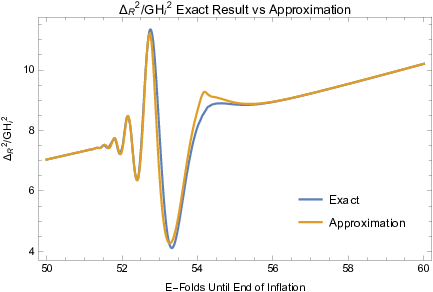
We should also point out that very accurate functional expressions are now available for the power spectra of single scalar inflation, valid to all orders in the slow roll parameter , and even including nonlocal effects from times before and after first horizon crossing [43, 44]. These expressions take the form [45],
| (14) | |||||
| (15) |
where the local slow roll correction factor is,
| (16) |
For the nonlocal corrections and it is best to abuse the notation by writing the first slow parameter as a function of , the number of e-foldings since the start of inflation,
| (17) | |||||
| (18) | |||||
Here , , and the functions of are,
| (19) | |||||
| (20) | |||||
| (21) | |||||
| (22) |
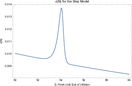
The confidence bound on the tensor-to-scalar ratio of [27, 28] implies , so is about a hundred times smaller than . Models with smooth potentials typically have and , so the leading contributions in come from the 3rd and 5th terms of expression (17). In particular the 5th (final) term is needed to correct for a systematic under-prediction of the local slow roll approximation [45]. For models with features the leading contributions to come from the 1st, 3rd and 4th terms of expression (17) [45]. These corrections can be very important for realistic models such as the one depicted in Figure 1.
To keep the analysis simple, we illustrate the procedure for predicting from using only the leading slow roll terms in expressions (14-15), without either of the nonlocal corrections or even the slow roll factor . The conversion from wave number to time is,
| (23) |
The leading slow roll approximation (14) for the scalar power spectrum can be recognized as a differential equation for the Hubble parameter,
| (24) |
We can integrate this equation from some arbitrary time to ,
| (25) |
Substituting the reconstructed Hubble parameter (25) into the leading slow roll approximation (10) for the tensor power spectrum gives,
| (26) |
Equation (26) is in some sense an integrated form of the single-scalar consistency relation (1) which can be applied more reliably. Both relations are valid to leading slow roll order, but whereas (1) compares a single value of the high quality data in with a derivative of the poor data on , our relation (26) combines a single measurement of the tensor power spectrum at with the high quality scalar data to predict what should be for other wave numbers. This seems to be a better way of exploiting the sparse data on which is likely to persist for some years after a first positive detection.
3 Comparison Using Simulated Data
It is illuminating to compare the single scalar consistency relation with the method we propose using simulated data. Let us suppose that the actual tensor power spectrum corresponds to single scalar inflation with , and which implies . We further suppose the simplest possible dependence,
| (27) |
where the scalar amplitude (at the tensor pivot ) is . Let us assume that the first positive detection of this tensor power spectrum consists of results for five binned wave numbers, the same as was in fact reported for the spurious BICEP2 detection [34]. To simplify matters we assume a linear relation for logarithms of the observed wave numbers, , and that each measurement of has the same 1-sigma uncertainty of . These numbers are roughly consistent with what BICEP2 actually reported [34]. Hence the detection consists of five observations obeying the relation,
| (28) |
where the are independent Gaussian random variables with mean zero and standard deviation . Table 1 simulates the five data points using a random number generator to find the .
| 1 | ||||
|---|---|---|---|---|
| 2 | ||||
| 3 | ||||
| 4 | ||||
| 5 |
Because the relation (27) is linear we can use least squares to determine the parameters. The least squares fit for data points obeying the relation (with ) is,
| (29) | |||||
| (30) |
Even in this general form it is obvious that expression (29) for represents a sort of average whereas expression (30) is a kind of numerical derivative. So we expect the fractional error on to be larger than that on . That becomes even more apparent when specializing to and ,
| (31) | |||||
| (32) |
Hence the simulated data of Table 1 implies a reasonably accurate reconstruction of the tensor-to-scalar ratio,
| (33) |
but a miserably inaccurate value for the tensor spectral index,
| (34) |
The resulting check of the single scalar consistency relation is not very sensitive,
| (35) |
Because of the large (but statistically allowed) positive fluctuation the measured tensor spectral index (34) does not even have the right sign!
| 1 | ||||
|---|---|---|---|---|
| 2 | ||||
| 3 | ||||
| 4 | ||||
| 5 |
We propose to instead use the much better measured scalar spectral index to predict the tensor spectral index, up to an integration constant, and then to compare the fluctuation of the observed data around this prediction. For the model in question this might amount to assuming predictions of the form,
| (36) |
where is (31) and is (33). Table 2 reports these predictions, along with the difference between each simulated observation and the associated prediction . Of course the parameter comes from the parameter through relation (33), so the final column of Table 2 represents four statistically independent measurements. The resulting estimate for the scatter between measurement and prediction is,
| (37) |
This is quite consistent with our assumed 1-sigma fluctuation of for each observation.
4 Discussion
Resolving the tensor power spectrum is crucial for the progress of inflation because it constrains the causative mechanism. This is already evident from the angst [52, 53, 54, 55] elicited by the increasingly tight bounds on the tensor-to-scalar ratio [56]. A positive detection at several different wave lengths has the potential to falsify entire classes of models. For example, any model in which inflation is driven by the potential of a minimally coupled scalar must obey relation (1) between and the tensor spectral index [17, 18, 19]. Unfortunately, relation (1) requires taking a derivative of , and the first generation of detections will probably be too sparse to provide a good bound because numerical differentiation makes bad data worse.
It makes more sense to integrate the high quality data we already possess for . If the leading slow roll expressions (9-10) are assumed then the prediction (26) from requires only a single integration constant from . (The same thing would be true even if the more accurate approximations (14-15) were employed [45].) Fixing this constant uses up one combination of whatever data we have for , leaving the scatter of the remaining data about the prediction as a legitimate test of single scalar inflation. Hence relation (26) is a sort of integrated form of the single-scalar consistency relation (1) which can be applied more reliably. Section 3 compares this sort of scatter test with checking for simulated data based on a hypothetical detection of at five wave lengths with fractional errors similar to those reported in the spurious BICEP2 detection [34]. Of course no massaging of poorly resolved data is going to extract a precision bound, but the scatter test seems clearly better.
Note that it is simple to adapt the scatter test to data fits. For example, the usual parameterization of the scalar data [22, 23, 24, 25] implies,
| (38) |
Here is the scalar amplitude, is the scalar spectral index, and is a fiducial wave number.
Finally, we can look forward to the day, in the far future, when the tensor power spectrum is well resolved. Then the sort of scatter test we propose could be employed to search for correlations between features in the two power spectra. For example, Figure 1 depicts the bump in the first slow roll parameter from a model [46, 47] introduced to explain the scalar power spectrum’s dip at and peak at [48, 49, 50, 51]. These features are caused by the way the scalar nonlocal corrections (17) depend upon derivatives of . The tensor nonlocal corrections (18) involve the same derivatives — although lacking the large factors of — so it is obvious there will be corresponding features [45]. Resolving this sort of correlation probes the functional relation between the two power spectra far more deeply than the single scalar consistency relation.
Acknowledgements
This work was partially supported by the European Union’s Seventh Framework Programme (FP7-REGPOT-2012-2013-1) under grant agreement number 316165; by the European Union’s Horizon 2020 Programme under grant agreement 669288-SM-GRAV-ERC-2014-ADG; by a travel grant from the University of Florida International Center, College of Liberal Arts and Sciences, Graduate School and Office of the Provost; by NSF grant PHY-1506513; and by the Institute for Fundamental Theory at the University of Florida. One of us (NCT) would like to thank AEI at the University of Bern for its hospitality while this work was partially completed.
References
- [1] R. Brout, F. Englert and E. Gunzig, Annals Phys. 115, 78 (1978). doi:10.1016/0003-4916(78)90176-8
- [2] A. A. Starobinsky, Phys. Lett. B 91, 99 (1980). doi:10.1016/0370-2693(80)90670-X
- [3] D. Kazanas, Astrophys. J. 241, L59 (1980). doi:10.1086/183361
- [4] K. Sato, Mon. Not. Roy. Astron. Soc. 195, 467 (1981).
- [5] A. H. Guth, Phys. Rev. D 23, 347 (1981). doi:10.1103/PhysRevD.23.347
- [6] A. D. Linde, Phys. Lett. B 108, 389 (1982). doi:10.1016/0370-2693(82)91219-9
- [7] A. Albrecht and P. J. Steinhardt, Phys. Rev. Lett. 48, 1220 (1982). doi:10.1103/PhysRevLett.48.1220
- [8] A. D. Linde, Phys. Lett. B 129, 177 (1983). doi:10.1016/0370-2693(83)90837-7
- [9] A. A. Starobinsky, JETP Lett. 30, 682 (1979) [Pisma Zh. Eksp. Teor. Fiz. 30, 719 (1979)].
- [10] V. F. Mukhanov and G. V. Chibisov, JETP Lett. 33, 532 (1981) [Pisma Zh. Eksp. Teor. Fiz. 33, 549 (1981)].
- [11] R. P. Woodard, Rept. Prog. Phys. 72, 126002 (2009) doi:10.1088/0034-4885/72/12/126002 [arXiv:0907.4238 [gr-qc]].
- [12] A. Ashoorioon, P. S. Bhupal Dev and A. Mazumdar, Mod. Phys. Lett. A 29, no. 30, 1450163 (2014) doi:10.1142/S0217732314501636 [arXiv:1211.4678 [hep-th]].
- [13] L. M. Krauss and F. Wilczek, Phys. Rev. D 89, no. 4, 047501 (2014) doi:10.1103/PhysRevD.89.047501 [arXiv:1309.5343 [hep-th]].
- [14] V. F. Mukhanov, H. A. Feldman and R. H. Brandenberger, Phys. Rept. 215, 203 (1992). doi:10.1016/0370-1573(92)90044-Z
- [15] A. R. Liddle and D. H. Lyth, Phys. Rept. 231, 1 (1993) doi:10.1016/0370-1573(93)90114-S [astro-ph/9303019].
- [16] J. E. Lidsey, A. R. Liddle, E. W. Kolb, E. J. Copeland, T. Barreiro and M. Abney, Rev. Mod. Phys. 69, 373 (1997) doi:10.1103/RevModPhys.69.373 [astro-ph/9508078].
- [17] D. Polarski and A. A. Starobinsky, Phys. Lett. B 356, 196 (1995) doi:10.1016/0370-2693(95)00842-9 [astro-ph/9505125].
- [18] J. Garcia-Bellido and D. Wands, Phys. Rev. D 52, 6739 (1995) doi:10.1103/PhysRevD.52.6739 [gr-qc/9506050].
- [19] M. Sasaki and E. D. Stewart, Prog. Theor. Phys. 95, 71 (1996) doi:10.1143/PTP.95.71 [astro-ph/9507001].
- [20] D. J. Brooker, S. D. Odintsov and R. P. Woodard, Nucl. Phys. B 911, 318 (2016) doi:10.1016/j.nuclphysb.2016.08.010 [arXiv:1606.05879 [gr-qc]].
- [21] G. F. Smoot et al., Astrophys. J. 396, L1 (1992). doi:10.1086/186504
- [22] G. Hinshaw et al. [WMAP Collaboration], Astrophys. J. Suppl. 208, 19 (2013) doi:10.1088/0067-0049/208/2/19 [arXiv:1212.5226 [astro-ph.CO]].
- [23] Z. Hou et al., Astrophys. J. 782, 74 (2014) doi:10.1088/0004-637X/782/2/74 [arXiv:1212.6267 [astro-ph.CO]].
- [24] J. L. Sievers et al. [Atacama Cosmology Telescope Collaboration], JCAP 1310, 060 (2013) doi:10.1088/1475-7516/2013/10/060 [arXiv:1301.0824 [astro-ph.CO]].
- [25] P. A. R. Ade et al. [Planck Collaboration], Astron. Astrophys. 571, A16 (2014) doi:10.1051/0004-6361/201321591 [arXiv:1303.5076 [astro-ph.CO]].
- [26] R. Adam et al. [Planck Collaboration], Astron. Astrophys. 586, A133 (2016) doi:10.1051/0004-6361/201425034 [arXiv:1409.5738 [astro-ph.CO]].
- [27] P. A. R. Ade et al. [BICEP2 and Planck Collaborations], Phys. Rev. Lett. 114, 101301 (2015) doi:10.1103/PhysRevLett.114.101301 [arXiv:1502.00612 [astro-ph.CO]].
- [28] P. A. R. Ade et al. [Planck Collaboration], arXiv:1502.01589 [astro-ph.CO].
- [29] K. Hattori et al., Nucl. Instrum. Meth. A 732, 299 (2013) doi:10.1016/j.nima.2013.07.052 [arXiv:1306.1869 [astro-ph.IM]].
- [30] J. Lazear et al., Proc. SPIE Int. Soc. Opt. Eng. 9153, 91531L (2014) doi:10.1117/12.2056806 [arXiv:1407.2584 [astro-ph.IM]].
- [31] A. S. Rahlin et al., Proc. SPIE Int. Soc. Opt. Eng. 9153, 915313 (2014) doi:10.1117/12.2055683 [arXiv:1407.2906 [astro-ph.IM]].
- [32] Z. Ahmed et al. [BICEP3 Collaboration], Proc. SPIE Int. Soc. Opt. Eng. 9153, 91531N (2014) doi:10.1117/12.2057224 [arXiv:1407.5928 [astro-ph.IM]].
- [33] K. MacDermid et al., Proc. SPIE Int. Soc. Opt. Eng. 9153, 915311 (2014) doi:10.1117/12.2056267 [arXiv:1407.6894 [astro-ph.IM]].
- [34] P. A. R. Ade et al. [BICEP2 Collaboration], Phys. Rev. Lett. 112, no. 24, 241101 (2014) doi:10.1103/PhysRevLett.112.241101 [arXiv:1403.3985 [astro-ph.CO]].
- [35] N. C. Tsamis and R. P. Woodard, Annals Phys. 267, 145 (1998) doi:10.1006/aphy.1998.5816 [hep-ph/9712331].
- [36] T. D. Saini, S. Raychaudhury, V. Sahni and A. A. Starobinsky, Phys. Rev. Lett. 85, 1162 (2000) doi:10.1103/PhysRevLett.85.1162 [astro-ph/9910231].
- [37] S. Capozziello, S. Nojiri and S. D. Odintsov, Phys. Lett. B 634, 93 (2006) doi:10.1016/j.physletb.2006.01.065 [hep-th/0512118].
- [38] R. P. Woodard, Lect. Notes Phys. 720, 403 (2007) doi:10.1007/978-3-540-71013-4_14 [astro-ph/0601672].
- [39] Z. K. Guo, N. Ohta and Y. Z. Zhang, Mod. Phys. Lett. A 22, 883 (2007) doi:10.1142/S0217732307022839 [astro-ph/0603109].
- [40] R. P. Woodard, Int. J. Mod. Phys. D 23, no. 09, 1430020 (2014) doi:10.1142/S0218271814300201 [arXiv:1407.4748 [gr-qc]].
- [41] N. C. Tsamis and R. P. Woodard, Class. Quant. Grav. 21, 93 (2003) doi:10.1088/0264-9381/21/1/007 [astro-ph/0306602].
- [42] M. G. Romania, N. C. Tsamis and R. P. Woodard, JCAP 1208, 029 (2012) doi:10.1088/1475-7516/2012/08/029 [arXiv:1207.3227 [astro-ph.CO]].
- [43] D. J. Brooker, N. C. Tsamis and R. P. Woodard, Phys. Rev. D 93, no. 4, 043503 (2016) doi:10.1103/PhysRevD.93.043503 [arXiv:1507.07452 [astro-ph.CO]].
- [44] D. J. Brooker, N. C. Tsamis and R. P. Woodard, Phys. Rev. D 94, no. 4, 044020 (2016) doi:10.1103/PhysRevD.94.044020 [arXiv:1605.02729 [gr-qc]].
- [45] D. J. Brooker, N. C. Tsamis and R. P. Woodard, arXiv:1708.03253 [gr-qc].
- [46] J. A. Adams, B. Cresswell and R. Easther, Phys. Rev. D 64, 123514 (2001) doi:10.1103/PhysRevD.64.123514 [astro-ph/0102236].
- [47] M. J. Mortonson, C. Dvorkin, H. V. Peiris and W. Hu, Phys. Rev. D 79, 103519 (2009) doi:10.1103/PhysRevD.79.103519 [arXiv:0903.4920 [astro-ph.CO]].
- [48] L. Covi, J. Hamann, A. Melchiorri, A. Slosar and I. Sorbera, Phys. Rev. D 74, 083509 (2006) doi:10.1103/PhysRevD.74.083509 [astro-ph/0606452].
- [49] J. Hamann, L. Covi, A. Melchiorri and A. Slosar, Phys. Rev. D 76, 023503 (2007) doi:10.1103/PhysRevD.76.023503 [astro-ph/0701380].
- [50] D. K. Hazra, A. Shafieloo, G. F. Smoot and A. A. Starobinsky, JCAP 1408, 048 (2014) doi:10.1088/1475-7516/2014/08/048 [arXiv:1405.2012 [astro-ph.CO]].
- [51] D. K. Hazra, A. Shafieloo, G. F. Smoot and A. A. Starobinsky, JCAP 1609, no. 09, 009 (2016) doi:10.1088/1475-7516/2016/09/009 [arXiv:1605.02106 [astro-ph.CO]].
- [52] A. Ijjas, P. J. Steinhardt and A. Loeb, Phys. Lett. B 723, 261 (2013) doi:10.1016/j.physletb.2013.05.023 [arXiv:1304.2785 [astro-ph.CO]].
- [53] A. H. Guth, D. I. Kaiser and Y. Nomura, Phys. Lett. B 733, 112 (2014) doi:10.1016/j.physletb.2014.03.020 [arXiv:1312.7619 [astro-ph.CO]].
- [54] A. Linde, doi:10.1093/acprof:oso/9780198728856.003.0006 arXiv:1402.0526 [hep-th].
- [55] A. Ijjas, P. J. Steinhardt and A. Loeb, Phys. Lett. B 736, 142 (2014) doi:10.1016/j.physletb.2014.07.012 [arXiv:1402.6980 [astro-ph.CO]].
- [56] P. A. R. Ade et al. [Planck Collaboration], arXiv:1502.02114 [astro-ph.CO].