The decay $\tau\rightarrow K^{0}K^{-}\nu_{\tau}$ in the extended Nambu-Jona-Lasinio model

The present paper finishes the series of works devoted to describing of $\tau$-decays in neutrino and two pseudoscalar mesons in the framework of the extended Nambu-Jona-Lasinio (NJL) model [1, 2, 3, 4, 5]. Indeed, recently, the widths of the decays $\tau\rightarrow(\pi,\pi(1300))\nu_{\tau}$ [6], $\tau\rightarrow(\eta,\eta^{\prime})\pi\nu_{\tau}$ [7], $\tau\rightarrow K^{-}\pi^{0}\nu_{\tau}$ [8], $\tau\rightarrow(\eta,\eta^{\prime})K^{-}\nu_{\tau}$ [9] were calculated by using this model without applying any additional arbitrary parameters. This approach differs the NJL model [5, 10, 11, 12] from some other phenomenological models used for describing such processes [13, 14, 15, 16, 17, 18, 19, 20, 21, 22]. As a rule, these models use the vector dominance method, chiral symmetry and series of arbitrary parameters which are different for various processes.

In the extended NJL model, the quark-meson interaction Lagrangian for pseudoscalar $K^{0,\pm}$, vector $\rho^{\pm}$ mesons and their first radially excited states takes the form:

where $q$ and $\bar{q}$ are the u-, d- and s- constituent quark fields with masses $m_{u}=m_{d}=280$MeV, $m_{s}=420$MeV [4],[23], $K^{0,\pm}$, $\rho^{\pm}$ are the pseudoscalar and vector mesons, the excited states are marked with prime,

$f\left(\vec{k}^{2}\right)=1+d\vec{k}^{2}$ is the form factor for description of the first radially excited states [1],[2], $d$ is the slope parameter, $\theta_{a}$ and $\theta_{a}^{0}$ are the mixing angles for the strange mesons in the ground and excited states

The matrices

The coupling constants:

where

$Z_{K}$ is the factor corresponding to the $K-K_{1}$ transitions, $M_{K_{1}}=1272$MeV [24] is the mass of the axial-vector $K_{1}$ meson, and the integral $I_{2}$ has the following form:

$\Lambda_{3}=1.03$ GeV is the cut-off parameter [4].

The all these parameters were calculated earlier and are standard for the extended NJL model [2, 4].

The diagrams of the process $\tau\rightarrow K^{0}K^{-}\nu_{\tau}$ are shown in Figs.1,2.

The amplitude of this process takes the form:

where $G_{F}=1.16637\cdot 10^{-11}$MeV^-2 is the Fermi constant, $V_{ud}=0.97428$ is the element of the Cabbibo-Kobayashi-Maskawa matrix, $l^{\mu}=\bar{\nu}_{\tau}\gamma^{\mu}\tau$ is the lepton current, $q=p_{K^{0}}-p_{K^{-}}$, $M_{\rho}=775.11\pm 0.34$MeV, $M_{\rho^{{}^{\prime}}}=1465\pm 25$MeV, $\Gamma_{\rho}=149.1\pm 0.8$MeV, $\Gamma_{\rho^{{}^{\prime}}}=400\pm 60$MeV are the masses and the full widths of the vector mesons [24].

The first term corresponds to the diagram with the intermediate $W$-boson, the second and third terms correspond to the diagrams with the intermediate vector mesons $\rho(770)$ and $\rho(1450)$. The numerical coefficients

where $a(\vec{k}^{2})$, $b(\vec{k}^{2})$ and $c(\vec{k}^{2})$ are the coefficients from the Lagrangian defined in (2).

The calculated branching of the process $\tau\rightarrow K^{0}K^{-}\nu_{\tau}$ is

The experimental value of this branching are

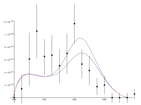
The mass and full decay width of the meson $\rho$(1450) are not defined precisely. It is interesting to note that if we choose the minimal values of mass and full width of this meson ($M_{\rho^{{}^{\prime}}}=1440$MeV, $\Gamma_{\rho^{{}^{\prime}}}=340$MeV), the results are in better agreement with the experimental data:

The comparison of the calculated and experimental differential width is shown in Fig. 3. The solid lines correspond to our theoretical differential width. The blue one is for the case of middle values of mass and full width of the meson $\rho$(1450), the red one is for the case of minimal values of them. The points correspond to the experimental values [25].

From two options considered in this paper, it is easy to see that the results are sensitive to the choice of the full decay width and mass of $\rho$(1450) meson. Since these mass and width are defined with the large errors, we can choose the minimal allowable values. This leads to better agreement with the experimental data. It is interesting to compare our results with the results from other phenomenological models and experiments. Such comparison is shown in Tab. 1. Our results are in satisfactory agreement with the experimental data.

We are grateful to A. B. Arbuzov and O. V. Teryaev for useful discussions.

References

• [1] M. K. Volkov, C. Weiss, Phys.Rev. D 56, 221 (1997)
• [2] M. K. Volkov, Phys.Atom.Nucl. 60, 1920 (1997) [Yad. Fiz. 60, 2094 (1997)]
• [3] M. K. Volkov, D. Ebert, M. Nagy, Int. J. Mod. Phys. A 13, 5443 (1998)
• [4] M. K. Volkov, V. L. Yudichev, Phys. Part. Nucl. 31, 282 (2000) [Fiz. Elem. Chast. At. Yadra 31, 576 (2000)]
• [5] M. K. Volkov, A. E. Radzhabov, Phys. Usp. 49, 551 (2006)
• [6] A. I. Ahmadov, M. K. Volkov, Phys.Part.Nucl.Lett. 12 (2015) 6, 744-750
• [7] M. K. Volkov, D. G. Kostunin, Phys.Rev. D86 (2012) 013005
• [8] M. K. Volkov, A. A. Pivovarov, Mod.Phys.Lett A31 (2016) 07, 1650043, arXiv:1511.08332 [hep-ph]
• [9] M. K. Volkov, A. A. Pivovarov, arXiv:1602.04970 [hep-ph]
• [10] M. K. Volkov, Sov. J. Part. Nucl. 17, 186 (1986) [Fiz. Elem. Chast. Atom. Yadra 17, 433 (1986)]
• [11] D. Ebert, H. Reinhardt, Nucl. Phys. B 271, 188 (1986)
• [12] D. Ebert, H. Reinhardt, M. K. Volkov, Prog. Part. Nucl. Phys 33, 1 (1994)
• [13] M. Finkemeier, E. Mirkes, Z.Phys. C 72, 619 (1996)
• [14] B. A. Li, Phys.Rev. D55 (1997) 1436
• [15] J. E. Palomar, FTUV-02-2102, IFIC-02-2102, arXiv:0202203 [hep-ph]
• [16] S. Nussinov, A. Soffer, Phys.Rev. D80 (2009) 033010
• [17] H. Czyz, A. Grzelinska, J. H. Kuhn, Phys.Rev. D81 (2010) 094014
• [18] S. Dubnicka, A. Z. Dubnickova, Acta Phys.Slov. 60 (2010) 1-153
• [19] N. Paver, Riazuddin, Phys.Rev. D84 (2011) 017302
• [20] D. G. Dumm, P.Roig, Phys. Rev. D 86, 076009 (2012)
• [21] R. Escribano, S. Gonzalez-Solis, M. Jamin, P. Roig, JHEP 1409, 042 (2014)
• [22] R. Escribano, S. Gonzalez-Solis, P. Roig, arXiv:1601.03989 [hep-ph]
• [23] M. K. Volkov, V. L. Yudichev, Eur.Phys.J. A10 (2001) 109-117
• [24] K. A. Olive et al. (Particle Data Group). Chin. Phys. C, 38, 090001 (2014) and 2015 update
• [25] CLEO Collaboration (T.E. Coan (Southern Methodist U.) et al.), Phys.Rev. D53 (1996) 6037
• [26] ALEPH Collaboration (R. Barate (Annecy, LAPP) et al.), Eur.Phys.J. C10 (1999) 1
• [27] Belle Collaboration (S. Ryu (Seoul Natl. U.) et al.), Phys.Rev. D89 (2014) no.7, 072009