The relaxation rate of a stochastic spreading process in a closed ring
Abstract
The relaxation process of a diffusive ring becomes under-damped if the bias (so called affinity) exceeds a critical threshold value, aka delocalization transition. This is related to the spectral properties of the pertinent stochastic kernel. We find the dependence of the relaxation rate on the affinity and on the length of the ring. Additionally we study the implications of introducing a weak-link into the circuit, and illuminate some subtleties that arise while taking the continuum limit of the discrete model.
I Introduction
In the absence of topology the relaxation time of a stochastic sample is determined either by the diffusion or by the drift, depending on whether the bias is small or large, respectively. In contrast, in a topologically closed circuit, as the bias is increased, the relaxation becomes under-damped with relaxation-rate that is determined by the diffusion and not by the drift. In related applications the “circuit” might be a chemical-cycle, and the “bias” is the so called affinity of the cycle.
In the present work we consider a minimal model for a topologically closed circuit, namely, an site ring with nearest-neighbor hopping. The dynamics can be regarded as a stochastic process in which a particle hops from site to site. The rate equation for the site occupation probabilities can be written in matrix notation as
| (1) |
If the ring were opened, then the limit would correspond to Sinai’s spreading problem [1, 2, 3, 4], aka a random walk in a random environment, where the transition rates are allowed to be asymmetric. Such models have diverse applications, notably in biophysical contexts of populations biology [5, 6] pulling pinned polymers and DNA unzipping [7, 8] and in particular with regard to molecular motors [9, 10, 11, 12].
In the absence of topology is similar to a real symmetric matrix, and the relaxation spectrum is real (aka damped relaxation). Alas, for a ring the affinity is a topological-invariant that cannot be gauged away, analogous to the Aharonov-Bohm flux, and the relaxation spectrum might become complex (aka under-damped relaxation). Thus the theme that we are addressing here is related to the study of of non-Hermitian quantum Hamiltonians [13, 14, 15]. In a previous work [16] we have illuminated the relation between the sliding-transition and the complexity-threshold, aka “de-localization transition”, as the affinity is increased.
The outline is as follows: In Sec.II we discuss the relaxation in the case of an homogeneously disordered diffusive sample, contrasting non-trivial topology (ring) with simple geometry (box). The effect of disorder is demonstrated in Sec.III, where heuristic considerations are used in order to explain the dependence of the relaxation rate on the affinity and on the length of the ring. In Sec.IV we discuss the delocalization transition. Namely, we find the threshold value of the affinity beyond which the relaxation becomes under-damped. Then we extract the relaxation rate from the characteristic equation using an “electrostatic picture”. As explained in Section V the same picture can be used in order to address sparse disorder. This motivates the analysis in Sections VI-VII of the relaxation in a ring that has an additional weak-link that forms a bottleneck for diffusion, though not blocking it completely. Several appendices are provided to make the presentation self-contained.
II Diffusive sample: Ring vs Box
The rate equation Eq. (1) involves a matrix whose off-diagonal elements are the transition rates , and whose diagonal elements are such that each column sums to zero. Via diagonalization one can find the eigenvalues . Irrespective of models details there always exists an eigenvalue that corresponds to the non-equilibrium steady state (NESS). The other eigenvalues reflect the relaxation modes of the system: they have positive , and might be complex. Complexity of the low eigenvalues implies an under-damped relaxation.
For a clean ring and with near-neighbor hopping, the rates are uniform but asymmetric, and are equal to for forward hopping, and for backward hopping. The matrix takes the form
| (2) |
with . Due to translational invariance, this matrix can be written in terms of momentum operator
| (3) |
From here it is easy to see that the eigenvalues are
| (4) |
The complexity of the eigenvalues implies that the relaxation process in not over-damped. A straightforward analysis of the time-dependent spreading process, see e.g. [17], shows that the drift velocity and the diffusion coefficient are given by the following expressions:
| (5) | |||||
| (6) |
where is the lattice constant. Note that in Eq. (3) we used the lattice constant as a unit of length (“”) else the following replacement is required: .
It is convenient to consider the continuum limit of the rate equation Eq. (1). In this limit we define and , and the continuity equation for the probability density becomes the Fokker-Planck diffusion equation:
| (7) |
One can easily find the spectrum of the relaxation modes () for either “ring” or “box” geometry. The length of the segment is , and the boundary conditions are respectively either of Neumann type or periodic. The result is
| (8) | |||||
| (9) |
where for the ring , while for the box . Clearly Eq. (8) is consistent with Eq. (4). The relaxation rate is determined by the lowest eigenvalue
| (10) |
For the “ring” it is determined solely by the diffusion coefficient:
| (11) |
while for the “box”, if the bias is large, it is predominantly determined by the drift:
| (12) |
It is important to realize that in the latter case we have a “gap” in the spectrum, meaning that does not diminish in the limit, hence the relaxation time is finite.
III Disordered ring
In the presence of disorder, the forward and backward rates across the th bond are random numbers and . Accordingly the diagonal elements of are random too, namely . By considering the long time limit of the time-dependent spreading process it is still possible to define the drift velocity and diffusion coefficient . The results depend in an essential way on the affinity of the cycle
| (13) |
where is defined via the sample average
| (14) |
Additionally it is useful to define threshold values , whose significance will be clarified in the next section, via the following expression:
| (15) |
Here, as in [17, 16] we assume that the rates are
| (16) | |||||
| (17) |
where the “activation energies” are box distributed within . Approximating the sample average by an ensemble average the thresholds of Eq. (15) are
| (18) |
For small one obtains , while in contrast the threshold is finite because the distribution of the “activation energies” is bounded.
The relaxation spectrum of a finite disordered sample (ring or box of length ) can be found numerically by solving the characteristic equation
| (19) |
The relaxation rate is defined as in Eq. (10). For a given realization of disorder we regard as a free parameter. Making larger means that all the are increased by the the same constant. We define the complexity threshold as the value beyond which the spectrum becomes complex. This means that for the relaxation is over-damped like in a box, while for the relaxation is under-damped like in a clean ring. It has been established [16] that
| (20) |
In the upper panel of Fig. 1 we calculate the dependence of on for a representative disordered ring via direct diagonalization of the matrix. The results are displayed as blue symbols. The complexity threshold Eq. (20) is indicated by the left vertical dashed line. In the lower panel of Fig. 1 we calculate the relaxation rate for a box configuration, i.e. one link of the ring has been disconnected. For such configuration the topological aspect is absent and therefore the spectrum of the site sample is real ().


We test whether Eq. (11) and Eq. (12) can be used in order to predict . For this purpose and are independently calculated using a standard procedure that is outlined in Appendix A of [17]. Indeed we observe in Fig. 1 a nice agreement between this prediction (solid and dashed green lines) and the previously calculated relaxation rate (blue symbols).
Having realized that of a ring is determined by via Eq. (11) we would like to understand theoretically the observed non-monotonic variation as a function of . In the limit the calculation of can be carried out analytically [2], using Eq. (77) of Appendix A. In this limit in the range where the spectrum is real; then it becomes infinite for , and finite for . The result of the calculation in the latter regime is represented by the red curve in the upper panel of Fig. 1. As expected it provides a good estimate only for large where Eq. (77) can be approximated by Eq. (78), leading to
| (21) |
Note that this expression roughly coincides with the clean ring result Eq. (11) with Eq. (6), see black curve in the upper panel of Fig. 1.
In the range the diffusion coefficient is large but finite and becomes dependent. In [17] a heuristic approach has been attempted in order to figure out this dependence. In the present work we would like to adopt a more rigorous approach. We shall deduce the dependence of analytically from the characteristic equation Eq. (19). We shall also provide an optional derivation for Eq. (21).

IV Extracting from the characteristic equation
With the of the rate equation Eq. (1) it is possible to associate a symmetric real matrix as explained in Appendix B. The latter has real eigenvalues with . Using the identity Eq. (88) of Appendix C, and setting the units of time such that , the characteristic equation Eq. (19) is
| (22) |
Taking the log of both sides, this equation takes the form . The identification of the right hand side as is based on the observation that has to be an eigenvalue, corresponding to the steady state solution. It is illuminating to regard as the complex potential in a two dimensional electrostatic problem:
| (23) |
where . The constant curves correspond to potential contours, while the constant curves corresponds to stream lines. The derivative corresponds to the field, which can be regarded as either an electric or a magnetic field up to a 90deg rotation. On the real axis (), the potential is
| (24) |
The spectral density of the eigenvalues is further discussed in Appendix D. Using the language of the electrostatic picture we regard it as a charge distribution. For full disorder the density for small is characterized by an exponent namely, . The spectral exponent is determined via Eq. (15). An explicit example for the implied dependence of on is provided by inverting Eq. (18). One observes that becomes infinite as approaches . For a gap is opened. In Appendix E we provide some insight with regard to the implied electrostatic potential . The bottom line is summarized by Fig. 2. For full disorder, if the envelope at the origin has a positive slope hence the equations has real solutions, and the relaxation spectrum comes out real. For the envelope at the origin has a negative slope, hence no real solutions at the bottom of the spectrum, and the low eigenvalues become complex. Accordingly the threshold for full disorder is determined by Eq. (20).
We would like to estimate the relaxation rate in the non-trivial regime , where the topology of the ring is reflected. Given the spectral density , the electrostatic potential is
| (25) |
Expanding to second order near the origin, we have
| (26) |
where the coefficients are defined as
| (27) |
Notice that and are the potential and the electrostatic field at the origin. To determine the real part of the complex gap it is enough to realize that the equipotential contour is approximately a parabola near the origin:
| (28) |
We define as a reference the field-line that stretches through the origin along the X axis to . The first excited eigenvalue is determined by the intersection of the potential contour with the next field line, namely with . By definition of the stream function , which can be regarded as an application of the Cauchy-Riemann theorem, it is equivalent to the requirement of having an enclosed flux
| (29) |
The integrand is approximated by , hence we deduce
| (30) |
If all the s are proportional to it follows that as in the case of a clean diffusive ring. This is indeed the case if . But if we have to be careful about the lower cutoff. From the quantization condition we deduce that and get
Comparing with Eq. (11) we realize that consistency requires to assume that for , and for . The latter result (but not the former) is in agreement with the heuristic approach of [17]. In the heuristic approach it has been assumed, apparently incorrectly, that the disorder-induced correlation-length scales like throughout the whole regime , and becomes size-independent for . Apparently the dependence of the disorder-induced correlation-length becomes anomalous within the intermediate range .
The result Eq. (IV) for has an obvious implication on the spectral density of the relaxation modes. Clearly with should be a function of , reflecting that the spectral density is extensive in . Accordingly Eq. (IV) can be re-phrased as saying that . This result is in general agreement with the heuristic argument of [12], but not in the regime , where it had been argued that . while our result is . The maximum difference is for . Our prediction is supported by the numerical example in Fig. 3. We also note that Eq. (28) implies that irrespective of . But a numerical inspection (not displayed) shows that the latter approximation works well only for the few first eigenvalues.
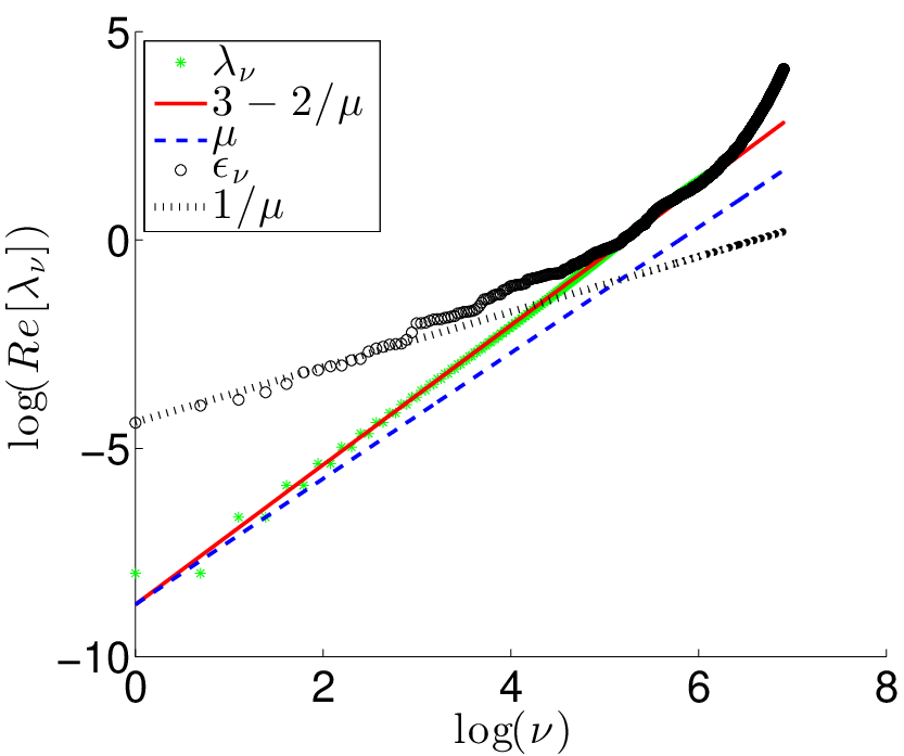
V Sparse disorder
So far we have considered “full disorder” for which one is able in principle to determine a coarse-grained diffusion coefficient , that may depend on , and from that to extract via Eq. (11), leading to Eq. (IV). But in practice the disorder might be “sparse” meaning that only a few links are defected. The extreme case is having a single “weak link”, meaning a bond or a region where the transitions are extremely slow. In such case Eq. (11) for , as well as Eq. (20) for are not physically meaningful. Still we can use the electrostatic picture of the previous sections in order to analyze on equal footing the secular equation. This will be demonstrated in the subsequent sections.
In order to get tangible analytical results we consider a minimal model, namely a diffusive ring with a single weak-link region. The length of the diffusive region is , and it is characterized by a diffusion coefficient , while the length of the defected region is , and it is characterized by a diffusion coefficient . We characterize the the weak link region by a “conductance” parameter , and take the limit keeping constant. We find that the threshold does not depend on as in Eq. (20), but rather reflects . The characteristic equation implies that as for a clean ring, but with a prefactor that depends on . This dependence is illuminating: it leads to an interpolation between the “ring” result Eq. (11) and the “box” result Eq. (12).
VI Ring with weak link
We would like to analyze how the relaxation spectrum is affected once a weak-link is introduced into a diffusive ring. We use the continuum limit Eq. (7) for the purpose of deriving the characteristic equation. In a region where and are constant a free-wave solution , has to satisfy the dispersion relation . It is convenient to use the notation , which would be consistent with the discrete-lattice convention if the lattice constant were taken as the unit length. Given we define that might be either real or pure-imaginary through the following expression:
| (35) |
The complex wavenumbers that correspond to this value are . In each location the actual stationary solution of Eq. (7) has to be a superposition of clockwise () and anticlockwise () waves
| (36) | |||||
| (37) |
We define the state vector
The transfer matrix that matches the state vector at two different locations is defined via the relation
| (45) |
In a ring with a weak-link there are two segments with different diffusion coefficients and . The continuity of the density and the current implies that the derivative should have a jump such that across the boundary
We define the matrices
For free propagation over a distance we have , with that involves a wavenumber that is determined by . For a weak-link we have , where describes the free propagation in the region that has some length . It is convenient to define the effective length of the weak link as . The only non-trivial way to take the limit of zero thickness weak-link () is to adjust such that is kept constant. This leads to the following result:
The characteristic equation is
| (65) |
leading to
| (66) |
where we have defined
| (67) |
along with and .


In Fig. 4 we find the dependence of the lowest eigenvalues on via numerical solution of Eq. (66) and using Eq. (35). The units of length and time are such that . From the first eigenvalue we get as defined in Eq. (10). It is implied by the re-scaling of the variables in the characteristic equation that as for a clean ring. In Fig. 5 we illustrate the dependence of on and on . The observed dependence is monotonic, unlike that of Fig. 1. In the clean-ring limit there is no dependence because we are considering the continuum-limit, setting irrespective of , while in Fig. 1 the diffusion coefficient was given by Eq. (6). Irrespective of this presentation issue, as decreases the drift-determined dependence is approached, in consistency with Eq. (12). Thus we have a nice interpolation between the “ring” and “box” expressions for .
In order to determine the threshold for the appearance of complex eigenvalues we take a closer look at Eq. (66). The left hand side is an oscillating function within an envelope
| (68) |
This envelope has a minimum at . Accordingly if complex eigenvalues appear, and we can deduce the threshold from the equation
| (69) |
To get an explicit expression we solve the approximated equation and deduce a solution in terms of the Lambert function,
| (70) |
This is valid provided , which is self-justified for small . We can use the same procedure in order to determine the complexity threshold for a given eigenvalue in Fig. 4. Recall that the corresponding is . Solving the quadratic equation we find the beyond which the spectrum becomes real again. It terms of the explicit expression is
| (71) |
This boundary is indicated by a dashed black line in Fig. 4).


VII Reconstruction of the continuum limit
By reverse engineering, requiring consistency between Eq. (66) and Eq. (22), we deduce that the electrostatic potential that is associated with the characteristic equation for a ring with a weak link is
| (72) |
This potential is plotted in Fig. 6, and labeled as “”. We would like to reconstruct this potential by means of Eq. (24). For this purpose we have to find the real eignevalues of the associated , see Eq. (85). Formally the equation is obtained by setting in the right hand side (RHS) of Eq. (66), leading to
| (73) |
From Eq. (35) it follows that , where are the roots of the above equation. Using these “charges” we compute via Eq. (24) and plot the result in the upper panel of Fig. 6. Some truncation is required, so we repeat the attempted reconstruction with and roots. We observe that the result converges to the limit. The residual systematic error as becomes larger is due to finite truncation of the number of roots used in the reconstruction.
The characteristic, equation Eq. (66) parallels the discrete version Eq. (22). One should be aware that the spectral density contains an “impurity” charge as illustrated in the third panel of Fig. 2. It is easy to explain the appearance of this exceptional charge using the discrete-lattice language. In the absence of a weak link the diagonal elements of the matrix are where . The spectrum of the associated matrix forms a band, such that the lower edge of is
| (74) |
If we introduce a weak-link at the bond, we get one exceptional diagonal element . Consequently, for small enough , there is an out-of-band impurity level that does not mix with the band:
| (75) |
In the lower panel of Fig. 6 we separate the contribution of the impurity level from the contribution off all the other band-levels.
VIII Discussion
We have outlined a physically appealing procedure to extract the relaxation rate of a stochastic spreading process in a closed ring, bridging between the discrete model and its continuum limit, and treating on equal footing full and sparse disorder. By sparse disorder we mean several weak-links. For presentation purposes we have provided a full analysis for a ring with a single defect, but the generalization to several weak links is merely a technical issue.
Our approach has been inspired by previous works regrding non-Hermitian Hamiltonians [13, 14, 15], and follows our previous publication [16] regarding the determination of the complexity threshold. In the present work the emphasis was on the determination of the relaxation rate in the “complex” regime where the topological aspect manifests itself. Generally speaking in this regime may exhibit anomalous dependence on the length of the sample.
Acknowledgements.– We thank Oleg Krichevsky (BGU) for a helpful discussion. This research has been supported by by the Israel Science Foundation (grant No. 29/11).
Appendix A Expressions for and in the presence of disorder
In the presence of disorder, the forward and backward rates are random numbers. Here we summarize known analytical expressions for and based on [2], and notations as in [17, 16]. Taking the infinite chain limit, and using units such that the lattice spacing is , the expression for the drift velocity is
| (76) |
We notice that a non-percolating resistor-network-disorder will diminish the drift velocity as expected due to the denominator. Irrespective of that the result above is valid only in the “sliding regime” where . Looking at the numerator one observes that the implied condition for that is . As for the diffusion, it becomes finite for , and the explicit expression is
| (77) | |||||
For large bias a practical approximation is
| (78) |
Considering a ring with random rates , the dependence of all the various expectation values on the affinity is expressible in terms of the parameters and . For example
| (79) |
Appendix B The associated matrix
Our model is described by a conservative matrix that describes hopping between sites. In the Chain configuration the site index runs from to , while in the Ring configuration it is defined modulo . In the latter case we characterize the stochastic field by a potential and by an affinity , such that
| (80) |
Then we associate with a similar matrix and a real symmetric matrix as follows:
such that
| (81) |
where is a diagonal matrix. The relation between and can be regarded as a gauge transformation, and can be regarded as an imaginary Aharonov-Bohm flux. The hermitian matrix can be regarded as the Hamiltonian of a particle in a ring in the absence of a magnetic flux. The of a clean ring Eq. (3) and its associated are
| (82) | |||||
| (83) |
while in the continuum limit Eq. (7) implies that
| (84) | |||||
| (85) |
In the absence of disorder the eignevalues are obtained by the simple substitution , where is an integer.
Appendix C The characteristic equation
Appendix D The spectral density
Consider a ring where the transition rates between neighboring sites are random variables . The equation that describes the relaxation in such a ring in the continuum limit is Eq. (7) with “white disorder”. Namely has Gaussian statistics with where . Assuming , and adding to the disorder an average value , one observes that the diffusion equation is characterized by a single dimensionless parameter. It is customary to define in consistency with Eq. (18)
| (89) |
This parameter equals if we use the common re-scaling of units such that . Then the units of time and of length are
| (90) | |||||
| (91) |
In the absence of disorder, by inspection of Eq. (85), the spectral density is like that of a “free particle” but shifted upwards such that the band floor is . In the presence of Gaussian disorder the gap is filled. In scaled units the integrated density of states is [3]:
| (92) |
where and are Bessel functions of the first and second kind. For any the large asymptotics gives in agreement with the free particle result. In the other extreme, for small we get . It is also not difficult to verify that the clean ring spectrum (with its gap) is recovered in the limit.
We have verified that for box-distributed the approximation holds at the vicinity of the band floor. In contrast with a Gaussian distribution becomes infinite as approaches , see Eq. (18). For a gap is opened.
Appendix E Step by step electrostatics
The eigenvalues of can be regarded as the locations of charges in a 2D electrostatic problem. We would like to gain some intuition for the associated potential along the real axis. For a point charge at we have . For a uniform charge distribution within we get
| (93) | |||
which has a minimum at and resembles a “soft well” potential. In order to have a flat floor the density has to be larger at the edges. This is the case for a charge density that corresponds to the spectrum of a clean ring. The locations of the charges are
| (94) |
and the potential along the real axis is
| (95) |
For within the band, the integrand can be written as , and accordingly the potential vanishes, reflecting an infinite localization length.
In the continuum limit the charge density in the case of a clean ring behaves as with and leads to a flat floor. For general one can show [16] that
| (96) |
such that the sign of is positive for , and negative for . See Fig. 2 for an illustration. We also illustrate there what happens if we have a clean ring that is perturbed by a defect that contributes a charge in the gap.
For we have , meaning that a gap is opened. If is sufficiently large the eigenstates of are “trivially localized”, so the eigenvalues are simply
| (97) |
where is uniformly distributed. Accordingly the charge density is within an interval , where and , leading to
| (98) | |||||
We would like to calculate the decay rate as described by Eq. (30). To carry out the calculation it is easier to integrate with respect to . Expanding Eq. (25) in the vicinity of the origin we get the coefficients
| (99) | |||||
| (100) | |||||
Substitution of and into Eq. (30) leads to a result that agrees with Eq. (21).
References
- [1] Y. G. Sinai, Theor. Probab. Appl. 27, 256 (1983), http://dx.doi.org/10.1137/1127028 .
- [2] B. Derrida, J. Stat. Phys. 31, 433 (1983).
- [3] J. Bouchaud, A. Comtet, A. Georges, and P. L. Doussal, Ann. Phys. 201, 285 (1990).
- [4] J.-P. Bouchaud and A. Georges, Phys. Rep. 195, 127 (1990).
- [5] D. R. Nelson and N. M. Shnerb, Phys. Rev. E 58, 1383 (1998).
- [6] K. A. Dahmen, D. R. Nelson, and N. M. Shnerb, in Statistical mechanics of biocomplexity (Springer Berlin Heidelberg, 1999) pp. 124–151.
- [7] D. K. Lubensky and D. R. Nelson, Phys. Rev. Lett. 85, 1572 (2000).
- [8] D. K. Lubensky and D. R. Nelson, Phys. Rev. E 65, 031917 (2002).
- [9] M. E. Fisher and A. B. Kolomeisky, P. Natl. Acad. Sci. USA 96, 6597 (1999).
- [10] M. Rief, R. S. Rock, A. D. Mehta, M. S. Mooseker, R. E. Cheney, and J. A. Spudich, P. Natl. Acad. Sci. USA 97, 9482 (2000).
- [11] Y. Kafri, D. K. Lubensky, and D. R. Nelson, Biophys. J. 86, 3373 (2004).
- [12] Y. Kafri, D. K. Lubensky, and D. R. Nelson, Phys. Rev. E 71, 041906 (2005).
- [13] N. Hatano and D. R. Nelson, Phys. Rev. Lett. 77, 570 (1996).
- [14] N. Hatano and D. R. Nelson, Phys. Rev. B 56, 8651 (1997).
- [15] N. M. Shnerb and D. R. Nelson, Phys. Rev. Lett. 80, 5172 (1998).
- [16] D. Hurowitz and D. Cohen, Scientific Reports 6, 22735 (2016).
- [17] D. Hurowitz and D. Cohen, Phys. Rev. E 90, 032129 (2014).
- [18] L. G. Molinari, Linear Algebra Appl. 429, 2221 (2008).