Automatic Theorem Proving in
Walnut
1 Introduction
Walnut is a software package that implements a mechanical decision procedure for deciding certain combinatorial properties of some special words referred to as automatic words or automatic sequences. To learn more about automatic words and their applications, see [2]. To learn about decision procedures for automatic words, see Schaeffer’s Master’s thesis [8] and the survey paper [9]. To read more about decidable properties of automatic words, refer to [4]. To read about another software package that provided a similar mechanical decision procedure for automatic words, and was developed before Walnut, read Goc’s Master’s thesis [7]. To see applications of Walnut, refer to [10, 11, 15, 13, 14, 12].
The aim of this article is to introduce Walnut and explain its core features. This article consists of four parts: basics, syntax, implementation, and the Walnut guide. In the first part, Section 2, we establish the basic notation and concepts. We go over words, automata, number systems, automatic words, and Presburger arithmetic. We learn what it means for an automaton to accept a predicate. We also learn how to automatically decide properties of automatic words.
The second part, Section 3, talks about the building blocks of predicates: constants, variables, operators, and different types of expressions. The semantics of predicates in Presburger arithmetic are well-known and are not explained, whereas semantic rules for calling and indexing, with which we extend the Presburger arithmetic to include automatic words, are explained in detail.
The third part, Sections 4 and 5, explains the decision procedure implemented in Walnut. The cross product of two automata, which is behind the construction of automata for all binary logical operators, is introduced. Building on that, we see how to construct automata for predicates from automata for subpredicates. In Section 5, we talk about two types of automata that do not appear often in Walnut, but are nevertheless important to understand.
The fourth and last part, Sections 6–8, starts with Walnut’s installation and goes over all of its commands, i.e., exit, eval, def, reg, and load. In Section 8, we learn how to manually define automata in text files. We also learn how to define new number systems.
If you are already familiar with the objects described in the first sentence of this introduction, you can skip Section 2 and come back to it only as a reference. For a more comprehensive treatment of the theory behind decision procedures for automatic words refer to [8, 9, 4].
Since this article is more about Walnut than the theory behind it, when we explain the latter, we use Walnut’s notation as opposed to the more familiar mathematical notation. For example, we use and for conjunction and universal quantifier as opposed to and of mathematical logic 11 1 Users enter logical predicates in a terminal when they use Walnut. We find that entering latex-like commands in the terminal, e.g., \forall, does not improve the readability.. As another example, when we define structures such as number systems or objects such as automatic words, we give the definitions that are closer to Walnut’s capabilities than the most general theoretical ones possible. This will help the reader make a smoother transition from the theory to its application in Walnut.
You can download Walnut from Jeffrey Shallit’s website, or alternatively from GitHub. Walnut is written in Java and is open source. It is licensed under GNU General Public License. We would appreciate it if users cite this article in their publications. For automata minimization Walnut relies on Valmari’s minimization algorithm [6]. In order to use this minimization algorithm in Walnut, we manually translated Valmari’s C++ implementation [5] almost varbatim to Java. For converting regular expressions to automata, Walnut relies on the automata library in [3]. We would greatly appreciate it if users report bugs to sh2mousa@uwaterloo.ca. The author would like to thank Jeffrey Shallit for revising this article.
2 Basics
2.1 Words and Automata
A word for a finite, infinite, or a possibly empty subset of natural numbers , is a sequence of symbols over a finite set called an alphabet. The set usually equals or for some . The set of finite and infinite words over the alphabet are denoted by and , respectively. The empty word is denoted by . For the finite word , the length , is defined and equals . We let denote the set of all words over of length . A subword (sometimes called “factor” in the literature) is a finite and contiguous subsequence of a word. The subword of starting at position of length is denoted by . Many interesting properties of words can be expressed in terms of their subwords. For example, the property of having two equal and adjacent subwords, referred to as a square, is discussed in numerous papers in the area of combinatorics on words. The product of two words and , denoted by , is the result of concatenating by .
There are cases where our words are defined over alphabets consisting of tuples of symbols, so let us fix our notation regarding these words. For a word over an alphabet , we let the projection map for denote the word over , obtained from by looking at the ’th coordinates, i.e., words are uniquely defined by
For example, for over we have and .
The reader is probably familiar with the notions of deterministic and nondeterministic finite state automata. In Walnut, an automaton with inputs (input tapes), is an -tuple , where is the (finite) set of states, is the initial state, is the set of final states, is the transition function, and is the alphabet of the ’th input (tape). The automaton’s alphabet is defined to be the cross product , and the notions of accepting a word or a language over this alphabet is defined as usual. A nondeterministic automaton is defined similarly, except that the transition function is defined by . In Walnut and throughout this article, the are finite subsets of integers .
Two automata are equal (isomorphic) if their underlying graphs are isomorphic. Two automata are equivalent if they accept the same language. There exists a determinization algorithm that converts a nondeterministic automaton to an equivalent deterministic automaton. There exists a minimization algorithm that converts an automaton to an equivalent automaton with the least number of states (which is unique up to isomorphism). It is known that extending the automata model by allowing multiple initial states (similar to how there can be multiple final states) does not add to the model’s expressiveness.
Next we extend the notion of accepting languages to relations, since the latter is more natural in Walnut:
Definition 1 (relations computed by automata).
The relation computed/accepted by is defined by
Since for every word , the words are all of the same length, the relation accepted by an automaton is consisted of tuples of the words of the same length, i.e., we have
For example, the language accepted by the following automaton is , whereas the relation accepted is :

In other words, the automaton accepts tuples where and are representations of the the same length, in the most-significant-digit-first binary system, of natural numbers and respectively. On the other hand, referring to the words in that are accepted by this automaton is not very descriptive. That is why, in this article, we prefer the relation (tuple) terminology over the language (word) terminology.
In almost all depictions of the underlying graphs of automata, such as the one in Figure 2.1, when a transition is not specified, it is assumed to be a transition to a dead state. In Walnut we do not store transitions to the dead state. Adding the dead state and all implicit transitions to it, is called totalizing an automaton.
An automaton with output is a tuple where are as before, the set is the output alphabet, and, instead of a set of final states, we have a map . The symbol is called the output of the state . An automaton with output can be thought of as an automaton that reads a word over and outputs whatever is the last state’s output. In Walnut, the output alphabet is a finite subset of integers. We can think of ordinary automata as a special case of automata with output by letting the set of final states to be . This is indeed how ordinary automata are stored in Walnut.
In the next section, we learn how to add more structure to alphabets by defining number systems. As we saw in the example, the automaton in Figure 2.1 accepts binary representations of numbers. In a moment we will extend our definition of automata to , where the are number systems and concealed in them are alphabets among other things.
2.2 Number Systems
In any course on theory of computation, it is customary to talk about the representations of the objects an algorithm/Turing machine takes as inputs. At the core of Walnut are automata taking natural numbers as inputs, and doing various computations on them, so fixing a representation for natural numbers is essential. We could limit ourselves to binary representations. However, there are many interesting automata accepting representations in number systems other than the binary one. So we are going to define, in general terms, the concept of a number system. Walnut allows number systems to be defined and used (with a few restrictions to the general definition below).
Definition 2 (number systems).
A number system is a -tuple of alphabet , language of valid representations containing and at least one of or , and decoding function that assigns integers to every word in and for which is usually written as . The decoding function has the following additional properties:
- •
if and only if
- •
- •
For all , either and for all , or and for all . The former is called an number system and the latter is called an number system22 2 and are short for most-significant-digit-first and least-significant-digit-first, respectively. However, it should not be taken literally in this definition, as one could define number systems (in the sense defined here), with no direct correspondence to the notion of most-significant-digit-first representation..
- •
For all positive , there exists for which and if is or if is . The word , if unique, is called the canonical encoding of in , and is sometimes denoted by . We let .
The addition relation is defined such that if and only if are of the same length and . The equality relation is defined such that if and only if and are of the same length and . The less than relation is defined as for which if and only if and are of the same length and . We adopt the in-order notation for , , and , i.e., we write , , and as opposed to the more cumbersome , , and respectively. It follows from the definition that for all , the set of representations of in , defined by is non-empty.
For example, the most-significant-digit binary system, denoted by , is defined by where
e.g., . For , we are very fortunate to have simple automata computing all of its important aspects, namely, valid representations , the addition relation , the equality relation , and the less-than relation . See Figures 2.2,2.3,2.4, and 2.5 respectively.
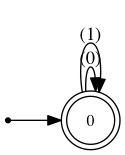
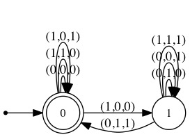
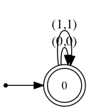
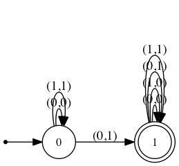
We can define the least-significant-digit-first binary system, denoted by , in a similar way. In fact, we can define and for all , and for all of them, there are simple automata computing valid representations, addition, equality, and less-than relations. In fact we can define the following:
Definition 3 (number systems in Walnut).
Number systems for which the automata for representations, addition, equality, and less-than exist, and equality is the same as word equality, i.e., if and only if , are exactly the type of number systems one can define and use in Walnut. Note that the alphabet of a number system is restricted to finite subsets of due to the same restriction on automata in Walnut.
In addition to base- number systems, Walnut has a built-in definition for the Fibonacci number system.
The most-significant-digit-first Fibonacci system, denoted by , is defined by where
where is the ’th Fibonacci number given by , and for . For example, . The set of valid representations is exactly the set of binary words avoiding consecutive s. The avid reader might want to verify that is a number system. There are automata computing all major aspects of . For example, here is the automaton accepting 33 3 The automaton accepting has states, which is too big to be represented here.:

In cases, where an automaton’s inputs are representations of integers in some number system, which by far are the most important type of automata in Walnut, we would like to signify these number systems instead of the input alphabets. For example, we might write to mean . It should be understood that in these cases, if for a word input is not a valid representation in , it does not mean that the automaton’s behavior is not defined for . This just means that is, by default, not going to get accepted. The behaviors of both automata and automata with output that are taking representations of numbers in some number systems as inputs are defined for all words (even those not representing numbers in the given number systems).
2.3 Automatic Words
An automatic word is a word in for which there exists a number system and an automaton with output for which reading outputs . In other words, for an automatic word, the symbol at position for all can be effectively computed by running an automaton with output on any single representation of in a number system. As usual we assume is a finite subset of .
The word for which the symbol at position , is the number of s in any binary representation of , modulo , is called the Thue-Morse word. The Thue-Morse word is well-defined since all the infinitely many different binary representations of an integer have the same number of ’s. It is instantly clear that is an automatic word over if one notes the automaton with output in Figure 2.7.

In the introduction, we mentioned that Walnut decides some properties of automatic words. Recall from Section 2.1 that squares are non-empty words of the form . It is easy to see that has square subwords. The following predicate captures this property:
Walnut provides a decision procedure that takes predicates like this and decides whether they are true or false. Walnut does so, by constructing automata for every subpredicate in the predicate above; see Section 2.4 for more details. It starts by constructing from the automaton in Figure 2.7 an automaton for subpredicate . This means (see Section 2.4) that is constructed so that it accepts tuples if and only if and substitutions , , and are satisfying . Walnut then using constructs an automaton for . The automaton takes two inputs representing the two free variables and in . Walnut continues by constructing the automaton for . In the end, Walnut returns true if accepts anything. The fact that ,, and exist is explained in Section 2.4. The details of how Walnut constructs these automata are explained in Section 4. The details of what comprises a valid predicate is explained in Section 3. To see more examples of the properties of the Thue-Morse word and their proofs see Section 7.1.
We can extend the definition of automatic words to higher dimensions. The (-dimensional) automatic word
is an infinite word over for which there exist number systems and an automaton with output
for which reading , such that for all , outputs
2.4 Automata accepting Predicates
In Walnut, we are interested in automaton accepting same-length representations in number systems of integers satisfying some predicate . When this is the case we say that automaton accepts the predicate (or equivalently accepts relation of tuples satisfying ). We already saw a few examples of such automata in Figures 2.1–2.6. From [1], also see [8], and as it will be proved again in Section 4, for predicate in Presburger arithmetic such an automaton always exists. Presburger arithmetic is the first-order theory of natural numbers, in which predicates are consisted of constants (natural numbers), variables over natural numbers, existential quantifiers, universal quantifiers, logical operators (conjunction, disjunction, negation, exclusive disjunction, implication, equivalence), arithmetic operators (addition, subtraction, multiplication and division by constants), and comparison operators (equality, less than, greater than, less than or equal, greater than or equal)44 4 Presburger arithmetic in its formal definition recognizes only a minimal subset of constants and operators: ,,,,,, but it is not difficult to show that all the other objects and operators we mentioned, e.g., multiplication by constants, does not add to the power of Presburger arithmetic and can be derived from that minimal set of objects. See Section 3.2 for more details. One thing to note here is that subtraction exists only when there exists a non-negative number for which ..
You can find the list of all operators in table 3.1. This list has three operators, namely, reverse ` ,indexing , and calling , that are not allowed in Presburger arithmetic. By indexing we mean indexing into an automatic word, e.g., writing things like ; see Section 3.6 for more details. In [9],[4],[8], and also in Section 4.6 we learn that extending Presburger arithmetic to include indexing is still decidable. In Section 3.7 we learn about calling and in Section 4.5 we learn that it is just a syntactic sugar and does not add to the power of the extended Presburger arithmetic (one that includes indexing into automatic words). We learn about reverse operation in Section 4.3. From here on, by “predicate” we mean a predicate over this extended Presburger arithmetic (extended to include indexing into automatic words) and until we see the proof in Section 4, we accept the fact that there exist automata accepting such predicates.
In Section 3 we formally define what constitutes a predicate, but first let us see a few examples:
- •
- •
- •
- •
We adopt the terminology of free variables from mathematical logic, i.e., a variable that is not bound to a quantifier (quantified). For example has no free variables, and can be regarded as a constant, in this case it is always true.
We have seen that, given a predicate , for any ordering of free variables and for every assignment of number systems to those variables, there exists an automaton accepting such a predicate, i.e., a tuple of same length words is accepted by if and only if the substitutions satisfy .
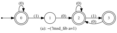
For example, consider the predicate . The automaton in Figure 2.1 accepts . Furthermore there exists automaton accepting tuples for which and substitutions , and are satisfying . There also exists an automaton accepting tuples for which and substitutions and are satisfying . By definition, both and also accept the predicate .
We would like to annotate predicates so that they contain information on number systems without ambiguity (we will see how shortly). For such an annotated predicate and the ordering on free variables, there exists a unique minimized automaton accepting the predicate. We denote this unique automaton by
The ordering we fix on variables, in Walnut and throughout this article, is the lexicographic ordering on the variables’ name.
The following are examples of annotated predicates55 5 Names for variables, words, and automata in Walnut start with a letter and can contain alphanumerics and underscores. So to distinguish number system annotations in a predicate we use the prefix .:
- •
- •
From the annotated predicate we understand that should all be interpreted in and should be interpreted as . Hence is the automaton accepting representations of and as its first and second inputs respectively. Also from annotation ?msd_fib in it is clear what to expect from automaton .
We can annotate a predicate with multiple number systems, e.g., see Figure 2.9. Here are the rules with which we assign number systems to constants, variables, and operators in a predicate:
- •
- •
If ?S appears outside all parentheses and brackets, then the number system is effective from the place it occurs in the predicate to the end of predicate.
- •
If none of the rules above applies, the number system is assumed to be by default.
- •
It is assumed that the number systems do not contradict each other, i.e., a single variable cannot have two different number systems in one predicate, and all operands of an arithmetic or comparison operator must belong to the same number system.
We saw in Figure 2.1, the unique automaton . In Figure 2.8, we see the automaton (recall that when the number system is not specified it is assumed to be ):

Note how this automaton fails to accept for any . This is obviously due to the fact that does not have a representation of length in . So we stress again that when we say automaton accepts predicate , we mean that accepts all (tuples of) equal length representations of satisfying . Therefore this example conforms to the definition.
Let us see an example of an automaton having multiple number systems. Figure 2.9 depicts the automaton .

3 Syntax and Semantic of Predicates in Walnut
3.1 Alphabets
We mentioned in earlier sections that all input and output alphabets of automata are subsets of integers in Walnut. Specifically for any automatic word , we can assume is an integer.
3.2 Arithmetic and Alphabetic Constants
Arithmetic constants in a predicate are allowed to be natural numbers only. There is, however, another type of constant: the alphabetic constant. Alphabetic constants are useful when referring to symbols at particular positions in automatic words. For example, the predicate that accepts positions for which the automatic word is is written as . In order to draw the distinction between alphabetic and arithmetic constants, we use alphabetic constants with a prefix of . The reason we call these constants alphabetic (as opposed to arithmetic) is due to the fact that Walnut does not allow (and it does not make much sense to allow) predicates that are comparing indexing expressions 3.6 and arithmetic expressions 3.5, e.g., expressions such as is not allowed. As we will see in Section 3.8, the only objects that can be compared with indexing expressions are alphabetic constants and indexing expressions themselves.
3.3 Variables
A variable’s name must start with a letter and can contain upper- and lower-case alphanumerics and underscores. A variable’s name cannot be E or A.
3.4 Operators
The full list of operators allowed in predicates can be found in Table 3.177 7 we prefer this notation to those familiar from mathematical logic, because we want to liken our notation to those of programming languages, as Walnut is ultimately a programming language.. This list has operator precedences. The lower this number is, the higher the precedence is. For example, multiplication by constant has the highest precedence. Parentheses override all precedences. All operators are associative from left to right, except for complement , reverse ` , quantifiers E and A, calling $, and indexing which are all associative from right to left.
| precedence | operator | explanation | examples |
|---|---|---|---|
| 1 | multiplication by a constant | and | |
| 1 | division by a constant | but not | |
| 2 | addition | ||
| 2 | subtraction | ||
| 3 | equality | ||
| 3 | != | inequality | |
| 3 | less than | ||
| 3 | greater than | ||
| 3 | <= | less than or equal | |
| 3 | >= | greater than or equal | |
| 4 | complement | ||
| 4 | ` | reverse | |
| 5 | conjunction | ||
| 5 | disjunction | ||
| 5 | exclusive disjunction | ||
| 6 | => | implication | |
| 7 | <=> | equivalence | |
| 8 | E | existential quantifier | or |
| 8 | A | universal quantifier | or |
| 9 | calling | ||
| 9 | indexing |
3.5 Arithmetic Expressions
The permissible arithmetic operators are . Equality is not an arithmetic operator. A constant expression is an expression involving only constants and arithmetic operators that evaluates to a natural number, e.g., but not nor . An arithmetic expression is defined recursively in the usual way:
- •
A constant expression is an arithmetic expression, e.g., ,,, but not .
- •
A variable is an arithmetic expression, e.g., ,etc.
- •
For arithmetic expression , the expression is also arithmetic.
- •
For arithmetic expression and both of and are arithmetic expressions.
- •
For variable and constant expression all of ,, and are arithmetic expressions.
- •
For arithmetic expression and constant expression all of , , and are arithmetic expressions.
An arithmetic expression on its own is not a predicate, and it is not meaningful to talk about an automaton accepting an arithmetic expression. For example, talking about an automaton accepting makes sense, while talking about an automaton accepting is not meaningful. Walnut reports an error if the user tries to construct an automaton for an arithmetic expression.
See Section 4.4 to see how Walnut constructs automaton for valid predicates like
where the and are variables or arithmetic constants, are arithmetic operators, and is a comparison operator.
3.6 Indexing Expressions and Their Semantic Rules
For an -dimensional automatic word , an indexing expression is where the are either arithmetic expressions or predicates with one free variable.
An indexing expression on its own is not a valid predicate, and it is not meaningful to talk about automata accepting indexing expressions. Smallest predicates involving indexing expressions are defined in Section 3.8 and they involve comparison operators.
We use indexing expressions to refer to positions indicated by . The semantic of predicates involving indexing expressions can be derived from the following rule:
Definition 4 (semantic rule regarding indexing).
Suppose automatic word , expressions where the are either arithmetic expressions or predicates with one free variable, free variables occurring in the , and an alphabetic constant are given. Predicate is satisfied by substitutions for all , if all of the following hold:
- •
If is an arithmetic expression, then is the value of the when evaluated at for all .
- •
If is a predicate with one free variable, then it is satisfied by substitutions for all . Let equals when is the free variable in .
- •
The symbol equals .
Having this rule, coming up with similar rules for other comparison operators, e.g., , and even predicates involving comparison of two automatic words, e.g., , should be straightforward. Recall that alphabetic constants are ordered just like integers.
3.7 Calling Expressions and Their Semantic Rules
For an automaton with inputs a calling expression is where the are either arithmetic expressions or predicates with one free variable. For such an expression, we say that is called with arguments . A calling expression on its own is a valid predicate, as we will see in Section 3.8.
Definition 5 (semantic rule regarding calling).
Suppose is the automaton for some predicate . Suppose expressions where the are either arithmetic expressions or predicates with one free variable, and free variables occurring in the are given. Predicate is satisfied by substitutions for all , if all of the following hold:
- •
If is an arithmetic expression, then is the value of when evaluated at for all .
- •
If is a predicate with one free variable, then it is satisfied by substitutions for all . Let equals when is the free variable in .
- •
is satisfied by substitutions for all .
3.8 Relative Expressions
Comparison operators are ,!=,,,<=, and >=. A relative expression is any of the following:
- •
An expression where and are arithmetic expressions and is any comparison operator.
- •
An expression where and are indexing expressions and/or alphabetic constants and is any comparison operator.
- •
A calling expression is a relative expression.
We stress that is not a relative expression based on the definition above, since is an indexing expression and is an arithmetic expression. We will see shortly that any relative expression is a predicate. Section 4.4 explains how to construct automata accepting relative expressions.
3.9 Predicates
A predicate is an expression formed from relative expressions and logical operators:
- •
Every relative expression is a predicate.
- •
For every predicate all of , and are predicates.
- •
For every predicate and all of , , , , are predicates.
- •
For every predicate and free variables both of and are predicates.
The semantic rules with which we assign true and false values to predicates defined here can be obtained by adding the semantic rules for indexing and calling to the well-known semantics of first-order logic and Presburger arithmetic.
4 Decision Procedure: Walnut’s Implementation
In this section, we learn about a procedure that takes a predicate and constructs an automaton accepting that predicate. The procedure explained here is what implemented in Walnut, and we shall call it the decision procedure.
For every defined number system, Walnut knows the automata for valid representations, addition, equality, and less-than predicates/relations. Every predicate is ultimately built out of these four predicates using logical operators. So we only need to explain the construction of automata for complex predicates from automata for simpler subpredicates. We start by explaining cross product in Section 4.1, which is the core object when constructing automata for predicates formed from binary logical operators, i.e., ,,,=>,<=>. Then we move on to quantification in Section 4.2, explaining the construction of automata for predicates formed from E and A operators. In Section 4.3, we discuss construction of automata for the complement and reverse ` operators. With these tools at our disposal, we are on the right track to construct automata for complex predicates formed from comparison and arithmetic operators, e.g., ,,,<=,etc. which we explain in Section 4.4.
4.1 Cross Product
Let and be the automaton and respectively. Let us assume that if then . Let where be the union of and and further assume that the are appearing in lexicographic order. Depending on whether or , let denote or respectively. Then the cross product of and denoted by is the tuple
where the transition function is defined to be
for equals or depending on whether or respectively. Note that is not an automaton since a set of final states is not specified. For , let denote the automaton .
Theorem 6.
For , the automaton accepts predicate . Furthermore, minimizing , we obtain automaton .
Proof.
Based on the definition for cross product, for to be defined, the same variables in and have to have the same number systems assigned in and . But that is exactly the same condition that needs to hold for number system annotations in to be consistent (in the sense defined in the last bullet in Page • ‣ 2.4).
Let and such that and where and are all equal and whenever . Let such that or depending on whether or .
We have the following equivalent statements:
- 1.
accepts .
- 2.
There is a path from to in reading .
- 3.
There is a path from to in reading , and there is a path from to in reading .
- 4.
accepts and accepts .
- 5.
is satisfied by substituting for all , and is satisfied by substituting for all .
- 6.
is satisfied by substituting .
∎
Obviously both the construction of cross product and minimizing automata can be carried out using algorithmic procedures. Therefore Theorem 6 gives us a procedure for constructing the automaton for conjunction.
With proper definitions for , we have similar theorems for when is any other binary logical operator.

Recall that transitions not depicted are transitions to a dead state. The cross product operation is depicted below:

Making a final state, minimizing, and renaming the states, we get the automaton in Figure 4.4.

4.2 Quantification
In this section we learn how to construct an automaton from automaton . Let be the automaton and let be the predicate . We first construct the nondeterministic automaton
from by eliminating the ’th input (coordinate) on all transitions, i.e., letting
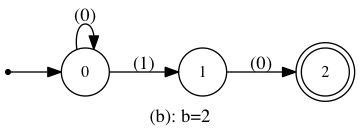
For example, letting be the automaton depicted in Figure 4.4, the automaton is depicted as follows:
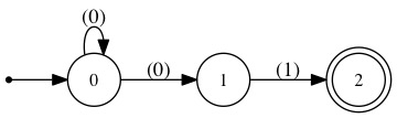
By the definition of transition function of , i.e., , it is easy to see that if accepts , then accepts
However, there might be where the are equal for all and substitutions for all , satisfies but does not accept . In other words, there are cases where does not accept .
In our example accepts for all , and as it is clear accepts for all . However does not accept , whereas should be accepted by any automaton accepting .
Therefore, we have to do more work on , to get to an automaton for . However as we will see in Lemma 1, the automaton might only miss an insignificant portion of accepted tuples of an automaton accepting . These insignificant tuples missed by are those with leading or trailing zeros. The good news is that with a little bit of technical work, it is possible to revive even these insignificant tuples.
Lemma 1.
Let ,,, and be as in the discussion above, and suppose is some tuple of same length words. If is satisfied with substitutions for , then there exists a constant and such that for all we have or depending on whether is or , and is accepted by . It is also the case that whenever for any , with the appropriate substitutions, is satisfying , then is also satisfying .
Proof.
Substitutions for satisfying predicate means that there exists a natural number , such that the substitutions above together with is satisfying the predicate . By definition of number systems, there exists a word such that . Also by definition of number systems for any integer and word , if we have , then either for all or for all depending on whether is or . Therefore there exists an integer such that is either or depending on whether is or and and for all . Therefore is accepted by where for all we have or depending on whether is or . Now by definition of , we know that is accepted by . This completes the first part of the lemma.
The second part follows very easily from the same properties of number systems mentioned in the proof of the first part of the lemma. ∎
Based on Lemma 1, to get we just have to construct an automaton from such that whenever for any is accepted, is also accepted. For the case where all for are either all or all , we can come up with an easy algorithm to revive tuples from . In case of all , let be the set of all states in reachable from the initial state by reading , or in case of all , let be the set of all states reaching to a final state by reading . We can compute or using breadth-first search. In the case of the nondeterministic automaton88 8 This is an automaton with multiple initial states. One can show that for every nondeterministic automaton with multiple initial states, there is an equivalent automaton with only one initial state.
and in the case of the nondeterministic automaton
is equivalent to . Determinizing and minimizing this automaton gives us .
In Figure 4.5, the variable is over . So the set is , therefore the following nondeterministic automaton accepts :
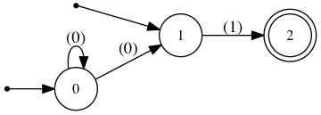
Now determinizing and minimizing this automaton gives us :
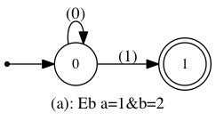
To obtain an automaton for , note its equivalence to , where is the logical complement (negation). See the next section to learn about the complement operator.
4.3 Complement and Reverse
To obtain from , one has to add all transitions to dead state (in Walnut, we call this totalizing an automaton), and then switching final and non-final states, but one also has to make sure that the resulting automaton is intersected with the automaton accepting where is the number system assigned to in (annotated) predicate . (Recall that is the set of all valid representations in the number system . Also recall that to define and use a number system in Walnut, one has to provide automaton accepting the set of all representations in that number system, therefore automaton accepting could be constructed easily using cross product explained in Section 4.1.)
Take a look at automaton depicted in Figure 4.8 that accept words representing in .

Now to obtain , we first add the dead state and all the transitions to it:

Switching final and non-final states we obtain an automaton accepting :

But then this automaton accepts words that have consecutive ’s which are not acceptable Fibonacci representations. So to get the final answer we have to intersect this automaton with the one depicted in Figure 2.6. The result is depicted in 4.11.
The reverse operator is not a logical operator per se, but we include it because it is useful when working with automata. The operand of the reverse operator is an automaton 99 9 Unlike the reverse operator, operands for logical operators are predicates. The reader however understands the very thin and superficial distinction between automata and predicates in this article.. The result is an automaton with all its transitions reversed.
4.4 Arithmetic and Comparison Operators
Recall that for every number system that we use in Walnut the three automata , 1010 10 This automaton does not need to be defined explicitly by the user, because we assumed for all number systems in Walnut if and only if ., and are defined. In this section we show that using these three automata and the decision procedure outlined in Sections 4.1–4.3, we can construct automata for more complex relative expressions with lots of arithmetic operators.
For a constant , a natural number, automata can be constructed recursively using automata and where is the predecessor of , i.e., . For example, predicate is equivalent to Similarly is equivalent to . Based on Definition 2, for all number systems , the automaton for is the simple automaton accepting . To construct automaton , just note that the predicate is equivalent to .
A similar recursive argument can be applied to obtain for a constant , i.e., one can construct where is the predecessor of . The similar argument can be applied to obtain automata for division by constants or subtraction.
To construct , note its equivalence to . With similar arguments, one can construct automaton for other comparison operators.
It is important to understand Walnut’s construction of
where . Here denotes an arbitrary comparison operator, and the are arbitrary arithmetic operators. Also let and be variables or arithmetic constants. All arithmetic operators in Walnut are associative from left to right; see Section 3.4. Based on this, Walnut first transforms the predicate to an equivalent predicate
Now Walnut has all the resources necessary to construct this last automaton.
For example, to construct , Walnut first transforms it to . The automaton is depicted below:
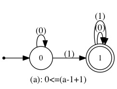
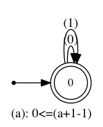
There is something here that is worth noting. Note how this automaton does not accept ? In arithmetic over integers satisfies the predicate. However in Presburger arithmetic setting gives , which is not acceptable, since Presburger arithmetic is defined over natural numbers. In order to fix this issue, try to always postpone subtraction and division to the rightmost position in your predicates. For example, writing results in
4.5 Calling an Automaton
In Section 3.7, we learned about the syntax and semantic of calling an automaton. A calling expression is a kind of syntactic sugar to save some space when writing long and complicated predicates. Suppose we already have computed the automaton and given it the name . We can refer to in a predicate without writing all over again, by just writing , where symbol is to signify that is an automaton, and the are either arithmetic expressions or predicates with exactly one free variable. In such case, we say, predicate is calling (or is calling predicate ).
To construct automaton for , Walnut constructs the equivalent automaton:
where are the free variables in , is the number of predicates in , are indices of predicates among , and if is an arithmetic expression, then , otherwise is a predicate, and is the free variable occurring in .
The fact that this predicate is equivalent to could be obtained easily using the semantic rule explained in Section 3.7. Walnut’s implementation includes some considerations to improve efficiency. For example, obviously when is a variable, we do not need to introduce a new variable .
The commands def and eval in Walnut are responsible for constructing the automaton from predicate . Unlike eval, the command def saves the automaton so it can be called later from other predicates like . See Section 7.2 for more information on def command.
To see an example, let be the automaton , and let be the predicate . The automaton in Figure 4.14 accepts .
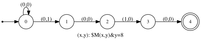
Please refer to Section 7.2, which is devoted to examples of calling automata.
4.6 Indexing an Automatic Word
Suppose is an -dimensional automatic word and is its corresponding automaton with output. Also let be an alphabetic constant. We note that is the automaton
when minimized, where . Similar arguments can be made for other comparison operators.
Suppose and are - and -dimensional automatic words, respectively, and let and be their corresponding automata with output. We note that is when minimized, where contains all where and are states of and , respectively, and they have the same output. Similar arguments can be made for other comparison operators.
5 Special Automata in Walnut
5.1 True and False Automata
In Section 2.4 we saw an example of a predicate with no free variables:
This predicate evaluates to true (it is a tautology). Here is an example of a predicate with no free variable that evaluates to false (contradiction):
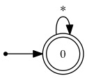
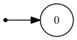
Walnut assigns a special automaton called true (false) automaton to predicates with no free variable that evaluate to true (false). However there could be predicates with free variables that are converted to true or false automata. See the following conventions implemented in Walnut:
- •
Conjunction (disjunction) of true automaton with automaton yields (true automaton, respectively).
- •
Conjunction (disjunction) of false automaton with automaton yields false automaton (, respectively).
- •
Negation of true automaton is false automaton and vice versa.
- •
Conventions for other logical operators follow from the above.
These conventions are reflecting the following facts from mathematical logic (for a predicate ):
- •
and are equivalent to and true respectively.
- •
and are equivalent to false and respectively.
- •
and .
As an example, the automaton is exactly the same as automaton . As another example, the automaton is the false automaton. As in our last example, note that is the true automaton.
5.2 Non-arithmetic Automata
There is a need for automata in which inputs (or some of them) do not represent numbers in a specific number system. These automata might accept patterns, or they might be relying on some non-arithmetic instructions.
For example, the pattern represents powers of in . However, the same pattern represents powers of in . Therefore, by not assigning a number system to the automaton accepting the pattern , we are allowed to call both in predicates in and in predicates in . Assigning number systems to automata accepting patterns usually does not make much sense. See more examples in Section 7.5.
Allowing non-arithmetic automata is specially helpful when working with the class of paperfolding words. These words are defined with an automaton that takes two inputs. One input is a number that represents a position in the paperfolding word and the other input is folding instruction that does not represent numbers. To see how Walnut can be used to prove properties of paperfolding words see [10].
6 Installation
Walnut is a command line program. You can run Walnut on any platform as long as you have Java 8 or later (preferably JDK 8 or higher) installed. To see which version of Java is installed on your machine type the following in the terminal (without the command line prompt $):
If you download Walnut as the zipped file Walnut.zip first thing you need to do is to uncompress it. Then open the terminal (or command prompt in Windows), and change the directory to “…/Walnut/bin/”, and run Walnut by typing:
To exit Walnut, type the following command (with the semicolon):
To make the distinction that we are typing a Walnut command, names of all Walnut’s commands are written in green. Walnut produces graphical representations of automata among other things. Those representations are files with .gv extensions. In order to open these files you need to install Graphviz, a graph visualization package which is available for all platforms. All text files that Walnut produces are in the UTF-8 encoding. All text files that Walnut reads have to be in the UTF-8 encoding as well. Most editors, e.g., vim, notepad, etc., use UTF-8 encoding by default.
6.1 Eclipse
As explained in the previous section, you can use the terminal to work with Walnut and enter your commands. However, I encourage you to use a Java IDE, like Eclipse, because in my opinion, entering commands in the console of a good IDE is more convenient than doing the same in the terminal. You are only going to run Walnut inside the IDE and use the IDE’s console (not the source code editor) to enter Walnut commands. Here is the instructions on how to run Walnut inside Eclipse for Java:
- 1.
Go to this link and download Eclipse for Java for your specific platform.
- 2.
Downloaded file is probably compressed. To start Eclipse, first uncompress the file, then click on the file named Eclipse.
- 3.
When you run Eclipse, it asks for a workspace address. Feel free to enter the path to your desired directory.
Now we need to import Walnut into Eclipse as a Java project:
- 4.
When in Eclipse, go to “File > Import … ”. In the dialog that opens up choose “General > Existing Project into Workspace”.
- 5.
In the dialog that opens up, click browse, find Walnut (that you downloaded and uncompressed in the Installation section) and press open. Then click finish.
- 6.
Close the Welcome page in your Eclipse window.
- 7.
On the "Project Explorer" (probably) on the left of your screen, you can see only one project (the one that you just imported). Click on it. Then click on “src”. Then double click on “prover.java”.
- 8.
You will see a green circle with a white triangle inside it. Click on it. This causes Walnut to run.
- 9.
You can enter your Walnut commands in the console window in your Eclipse. If you are not able to find the console window, go to “Window > Show View > Other > General > Console” to open it.
7 Commands
Every command ends in either a colon, double colon, or a semicolon. If you want to see the reports on the intermediate steps of a computation use colon or double colon, otherwise use semicolon. For example, if we type:
we get an output similar to the following written in the console:
which explains that the automaton for predicate has 2 states and it took 2 milliseconds to compute it. We use blue to denote predicates. Here we use grey to indicate the output produced by Walnut in the console. We use red to indicate errors in the console.
Walnut prints to console only the major steps of a computation when a single colon is used to end a command. Use two colons if you want to see all the steps behind the scene (cross product 4.1, quantification 4.2, minimizations, converting NFAs to DFAs (determinizations), etc.):
then we get an output similar to the following written in the console:
Whitespace is ignored. You can, for example, span one single command into multiple lines to improve readability. So, for example, you can write the following interchangeably:
In case we forget to separate the name test and predicate of the eval command, Walnut catches it by returning an error:
Here is the full list of commands in Walnut and we will go over them one by one in detail:
- •
exit
- •
eval <name> <predicate>
- •
def <name> <predicate>
- •
macro <name> <template>
- •
reg <name> <number system> <regular expression>
- •
reg <name> <alphabet> <regular expression>
- •
load <file name>
7.1 eval: eval <name> <predicate>
This is the most important command in Walnut and it stands for “evaluate.” This command takes two arguments. The first argument is a name for the evaluation. Name of the evaluation starts with a letter and could contain alphanumerics and underscore. The files generated as the result of the eval command, all share the name given in the first argument. The second argument is a predicate that we want to evaluate. Predicates are always placed between quotation marks. To see the definition for predicates see Section 3.9. In this article we typeset predicates in math mode in LaTeX. However, the reader should note that this typesetting is different from the one they see in the terminal. Let us see an example:
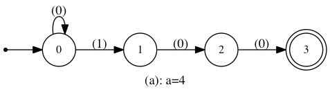
This evaluates to an automaton with one binary input labeled . This is the automaton . To learn about the notation see Section 2.4. The automaton accepts only if is the most-significant-digit-first binary representation of , i.e., if it belongs to . This automaton is drawn and saved in the directory “/Walnut/Result/” in a file named four.gv as shown in Figure 7.1. The graph drawing software Graphviz is required to open this file; see Section 6.
How does Walnut know to use the most-significant-digit-first binary system? Walnut defaults to which is how we show the most-significant-digit-first binary system in Walnut; see Section 2.2 to learn about this notation and to learn about number systems in general. To explicitly mention type:
Similarly, for the least-significant-digit-first binary type:

Here is another example, this time in :
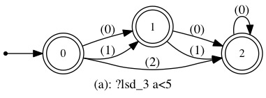
This automaton accepts exactly those words representing the numbers ,,,,and in the least-significant-digit ternary base, i.e., ,,,, respectively. Note the trailing zeros in the representations as opposed to the leading zeros in a most-significant-digit-first () number system. Also note that this automaton accepts the empty word. This is because in the definition of number systems we agreed that the empty word represents .
Let us see an example of an automaton with inputs:
This constructs the automaton in which the first input corresponds to , and the second input corresponds to . Recall from Section 2.4 that Walnut uses lexicographic ordering on the name of variables when constructing automata. So, for example, even though the first variable that appears in is , it corresponds to the second input in the automaton.
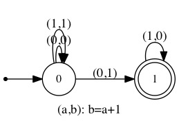
Walnut generates two other files as the outcomes of the eval command which can also be found in the directory “/Walnut/Result/”. For the evaluation two_inputs, these two files are named two_inputs_log.txt and two_inputs.txt and they are both text files.
The file two_inputs_log.txt contains the details of the evaluation including the intermediate steps and the time each of those steps took to complete. In our example, there are not many intermediate steps involved:
⬇ : 3 states - 0ms total computation time: 0ms
In addition to two_inputs_log.txt , another file with the name two_inputs_detailed_log.txt will be created if the command ends in two colons instead of a colon or a semicolon.
The file two_inputs.txt contains the definition of the automaton in Figure 7.4:
⬇ 1 msd_2 msd_2 2 0 0 3 0 0 -> 0 4 0 1 -> 1 5 1 1 -> 0 6 1 1 7 1 0 -> 1
Line indicates that the first and the second inputs of the automaton are both in . The two states and in Figure 7.4 are declared in Lines and . The first zero in Line refers to the state and the second zero refers to its output. Likewise, the first one in Line refers to the state and the second one refers to its output. Note that the automaton for evaluation two_inputs is not an automaton with output, however all automata are stored as automata with outputs in Walnut; see Section 2.1. For an ordinary automaton, states with non-zero outputs are interpreted as final states, and states with zero outputs are interpreted as non-final states. So here state is non-final, whereas state is final. Transitions for states and are declared in Lines - and respectively. For example, state on transitions to itself, and on transitions to state . Transitions not depicted are transitions to the dead state. For example, state transitions to the dead state on every tuple except . To learn more about definition of an automaton in text files and how to manually define automata in text files see Section 8.1.
In Section 2.3, we talked about the Thue-Morse word. The Thue-Morse word’s corresponding automaton with output, depicted in Figure 2.7, is defined in directory “/Walnut/Word Automata Library/” in a file named T.txt. We can refer to the Thue-Morse word in predicates by typing . See Section 8.2 on how to define new automatic words in Walnut.
We talked about square subwords in the Thue-Morse word. The following predicate is satisfied by if , i.e., if there exists a square subword of length starting at position .
The order of a square is half its length. Now if we want to find all natural numbers for which there exists a square of order in the Thue-Morse word, we simply use the existential quantifier E:

Based on this automaton, the natural number with representation of the form is an order of a square in the Thue-Morse word. In other words, the set of orders in the Thue-Morse word is
Overlaps are the words of the form where is a symbol and is any word, e.g., the word “alfalfa” in English is an overlap. It is a known that the Thue-Morse word avoids overlaps. How do we make sure, using Walnut, that the Thue-Morse word does not have any overlaps? The result of the following predicate must be the true automaton; see Section 5.1, if the Thue-Morse does not have any overlaps:

Note that if a predicate is not valid Walnut returns an error:
To understand why this is not a valid predicate see Section 3.5. In the following examples note how Walnut points to the locations of the errors in the predicates. By saying "char at ", Walnut tries to convey that there is something wrong going on at the vicinity of the ’th character in the predicate.
The last example can be fixed as follows:
To understand why see Section 3.8.
The last thing to note about the eval command is that Walnut overrides the files generated by an evaluation if the name of the evaluation is used in a new evaluation.
7.2 def: def <name> <predicate>
The word def stands for define. The syntax for this command is exactly the same as the syntax for eval command. The only difference between this command and eval is that the automaton constructed is saved in the directory “/Walnut/Automata Library/” for later use. Suppose we write the following:
This creates as usual the files sum10.gv, sum10.txt, and sum10_log.txt in the directory “/Walnut/Result/”. However, it also saves a copy of sum10.txt in the directory “/Walnut/Automata Library/”. Any automaton saved in this directory can be called in other predicates by referring to its name and the special character $. To learn about calling see Sections 3.7 and 4.5.
Let us see examples of predicates calling the automaton sum10:
This predicate is satisfied by numbers for which there exist an such that , i.e., :

We can send the same variable to both arguments of sum10:
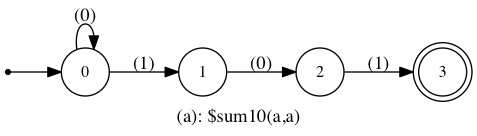
We can send constants to any arguments of sum10:
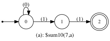
Indeed, we can send any arithmetic expressions or predicates with one free variable to arguments:
The resulting automaton for both of these is depicted in Figure 7.11. We can call sum10 to define new automata:
Now we can write
The result of this evaluation is again depicted in Figure 7.11.
Now look at the following example:
This is because the first argument is a predicate with two free variables.
We cannot send a variable in to an automaton that accepts only , and expect getting anything interesting in return. The following example would run fine, but the result is another nonsense:

The number of arguments when calling an automaton should match the number of inputs of that automaton:
Always remember the roles of the inputs to an automaton created by the def command. For example, look at the following examples of the def command:
Now the following evaluates to an automaton accepting representations of numbers :
whereas the following evaluates to an automaton accepting representations of numbers :
This is because f1 is an automaton for which the first argument is greater than the second argument, whereas, f2 is an automaton for which the first argument is less than the second argument. Always remember that Walnut sorts inputs of an automaton based on their labels’ lexicographic order.
7.3 macro: macro <name> <template>
Recall that a subword is a palindrome if for all . The following calculates the palindromes in the Thue-Morse word1111 11 In specific terms, this calculation constructs an automaton accepting ’s for which is a palindrome.:
Now in order to calculate palindromes for the Fibonacci word, one has to type the entire predicate above, letter for letter, except for the substitution of by :
There are many other example where one would like to calculate the same calculation for many different words. Similar to the def command, the macro command is a mechanism for avoiding dull repetitions. For the palindrome example, one could define the following macro:
This command saves the template ?\%0 Ak k<n => \%1[i+k] = \%1[i+n-1-k] in a file named pal.txt in the directory “/Walnut/Macro Library/”. Then to calculate palindromes for the Thue-Morse word, using a similar syntax to function calls, one could write:
The first step in computing eval and def commands is a preprocessing task in which all macros will be replaced by their template strings. In our example, Walnut replaces the #pal(msd_2,T) by the template, saved in the file pal.txt, then substitutes %0 and %1 by msd_2 and T, respectively. Now see how easily one can calculate plaindromes for the Fibonacci word:
The important difference between the macro and the def commands is that the macro takes a template and stores it unaltered as a string, whereas the def command takes a predicate and stores the automaton calculated for that predicate. The macro saves the user from typing the same template over and over, while the def command saves the user from calculating the same predicate over and over.
Let us see a second example. An important automaton for any word is one that accepts triples for which subwords of length starting at positions and are the same. This automaton, which we call factoreq, shows up in many different calculations, a notable one being border calculation. Recall that has a border of length if subwords and are equal. In other words, the has a border of length if factoreq accepts . In Walnut, for Thue-Morse, this is the same as writing:
Now to calculate for Fibonacci, this becomes:
Using macros, one could capture the essence of the above calculations as follows:
With these macros at hand, one can calculate factoreq and border for many different words. For example, for Thue-Morse the calculation becomes:
and for the Fibonacci it becomes:
7.4 Matrices with eval and def
We postponed discussing the exact syntax of the eval and def commands until this section. These two commands can take an optional argument:
- •
eval <name> <space separated list of free variables>? <predicate>
- •
def <name> <space separated list of free variables>? <predicate>
The question marks are representing the fact that the corresponding arguments are optional. When a list of free variables is preset, in addition to the ordinary computation, Walnut will calculate the incidence matrices of the underlying graph of the computed automaton, corresponding to the transitions labeled by the listed free variables. It stores the matrices in the Maple syntax in a .mpl file in “/Walnut/Result/” directory.
Suppose is the automaton calculated for the predicate . For a free variable and a value , we let denote the matrix where the entry 1212 12 denotes the entry at th row and th column., for every pair of states and , is the number of tuples transitioning from to with in the ’th coordinate, or more formally
We already saw in Figure 7.4 an automaton accepting . Now writing
causes Walnut to calculate the matrices and :
In the same command, we could ask Walnut to calculate the incidence matrices for as well as by writing:
There are a lot of interesting things one can do using incidence matrices. For example for Fibonacci word, and Sturmian words in general, the number of distinct subwords of length , i.e., subword complexity, is . Now can one verify this using Walnut? The answer is yes. Please refer to [14] for this and a lot of other interesting applications.
7.5 reg
The word reg stands for regular expression. Before we talk about this command in detail, let us motivate the need for it through an example. Suppose we need an automaton accepting representations of powers of that are less than . There is no straightforward way of constructing an automaton accepting representations of powers of using eval and def commands1313 13 The set of powers of is not expressible in Presburger arithmetic. However the extended Presburger arithmetic that involves automatic words is powerful enough to express this set (why?). Remember how def command saves automata definition in directory “/Walnut/Automata Library/”? We can manually create a file power2.txt in this directory and write in it the definition of an automaton accepting binary representations of powers of :
⬇ 1 msd_2 2 0 0 3 0 -> 0 4 1 -> 1 5 1 1 6 0 -> 1
See Section 8.1 to learn the syntaxes of defining an automaton in a text file. Now we can write a predicate for powers of that are less than :

The better approach to this problem is to use the reg command. This command can be used in two different ways:
- 1.
reg <name> <number system> <regular expression>
- 2.
reg <name> <alphabet> <regular expression>
To construct an automaton that accepts representations of powers of we can use the first syntax:
Similar to eval and def command, the second argument is a name. The third argument is a number system, and the last argument is a regular expression. This will construct an automaton for the regular expression, and saves the result in a file named power2.txt in “/Walnut/Automata Library/”, in addition to saving, as usual, the drawing of the automata in power2.gv in directory “/Walnut/Result/”. The file power2.txt is exactly the same as File 7.13.
Note that is also the representations of powers of . For this reason, there needs to be a way of defining an automaton from a regular expression that is not restricted to a particular number system. We call such an automaton a non-arithmetic automaton; see Section 5.2. To create a non-arithmetic automaton accepting a pattern we can use the second version of the reg command in which instead of a number system we specify an alphabet:
The file general_power2.txt generated by this command is the following:
⬇ 1 {0,1} 2 0 0 3 0 -> 0 4 1 -> 1 5 1 1 6 0 -> 1
The only difference between Files 7.13 and 7.15 is the first line; see Section 8.1 for more information.
Since general_power2 is not restricted to a particular number system both of the following are valid:
Note that is also and representations of powers of for any . So what if we write the following:
Here Walnut is complaining about the fact that ’s alphabet is , whereas general_power2’s input alphabet is ; see File 7.15. Walnut is very strict about matching alphabets, which we understand is sometimes a drawback, for example in the above example. We will improve this feature in future releases of Walnut.
We use the automata library in [3] for converting regular expressions to automata. To see the syntax for regular expressions refer to this website.
Here is a summary of the important syntax:
| zero or more occurrences of an expression | |
|---|---|
| one or more occurrences of an expression | |
| union, e.g., | |
| . | any single character, e.g., |
| character class, e.g., means any of | |
| complement of a character class, e.g., is any of |
The alphabet in the second version of reg command could only be a subset of . Therefore the following is not allowed:
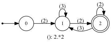
The last thing to note about the reg command is that for any regular expression , the resulting automaton from reg command is the intersection of the automaton for with where is the alphabet given as the third argument of the reg command. For example:
7.6 load: load <file name>
We can write any series of legitimate Walnut commands in a text file and save it in the directory “/Walnut/Command Files/”. Then we can load it by writing the following in Walnut:
This runs all commands in file_name.txt in the order they appear. Recall that the file’s encoding must be UTF-8.
8 Working with Input/Output
Throughout this section it is assumed that all files have UTF-8 encoding. This is the default encoding for most text editors.
8.1 Defining Automata in Text Files
In this section we learn how to manually define all automata types in text files. Recall that an ordinary automaton can be thought of as an automaton with output, in which states with non-zero outputs are treated as final states; see Section 2.1. Therefore suppose is an automaton with output with states and inputs over number systems . Furthermore suppose that the states are labeled to , i.e., , and that 1414 14 If an automaton does not follow these criteria we can always come up with an isomorphic one that does.. To define in a text file, first create a text file M.txt1515 15 File names in Walnut start with letters and can contain alphanumerics and underscore.. The first line must be
which declares inputs’ number systems. The second line is declaring state as follows:
where . Next lines are declarations of transitions of state which can come in any order. For every transitions are of the following form
whenever . There is no need to declare transitions to a dead state. For any pair that no declaration of the form above is mentioned, it is assumed that is a dead state. We can use , the wildcard matching symbol, in place of any symbol . If there is a transition of the form
it is understood that for every . After transitions of the state are declared, we declare state followed by its transitions. We continue like this until all states and their transitions are declared. Note that nowhere in M.txt we are defining the output alphabet . The output alphabet is inferred indirectly by looking at the state declarations. To see examples refer to Files 7.6–7.15.
A non-arithmetic automaton is defined in the same way, except that in the first line, for inputs that do not have number systems associated with them, we write down the alphabet between curly brackets. Alphabets can be any subset of integers. As an example see File 7.15.
Defining true or false automata in text files is easy. They have only one line and it is either true or false.
As one last example, the paperfolding words are given by the following automaton; see Section 5.2 and article [10] for more details:

This automaton is defined in the file PF.txt in directory “/Walnut/Word Automata Library/”:
⬇ 1 {-1,1} lsd_2 2 3 0 0 4 * 0 -> 0 5 1 1 -> 1 6 -1 1 -> 2 7 8 1 1 9 * 1 -> 4 10 * 0 -> 3 11 12 2 -1 13 * 0 -> 4 14 * 1 -> 3 15 16 3 1 17 * * -> 3 18 19 4 -1 20 * * -> 4
8.2 Defining New Automatic Words
The eval and def commands always produce automata accepting a predicate, therefore the result is never an automaton with output. So to define an automatic word , we need to manually define its corresponding automaton with output in the directory “/Walnut/Word Automata Library/”. For example, the Thue-Morse word is defined in the file “/Walnut/Word Automata Library/T.txt” as follows:
⬇ 1 msd_2 2 0 0 3 0 -> 0 4 1 -> 1 5 1 1 6 0 -> 1 7 1 -> 0
8.3 Defining New Number Systems
Based on Definition 3, to define a new number system , we need to define automata for , , and . We do not need to define an automaton for , because it can be generated easily, since we assumed that if and only if for any two words and of the same length. The automata for number systems must be defined in the directory “/Walnut/Custom Bases/”. For example, for the number system , assuming it is , one needs to create msd_S.txt, msd_S_addition.txt, and msd_S_less_than.txt for , , and respectively. If is , file names must be lsd_S.txt, lsd_S_addition.txt, and lsd_S_less_than.txt respectively. The number system defined in this way can be used in predicates by typing ?msd_S or ?lsd_S depending on whether is or . If the automaton for is not defined by the user, Walnut assumes that is the lexicographic ordering, i.e., if and are of the same length, then if and only if comes before in lexicographic order1616 16 Lexicographic ordering on symbols is assumed to be .. If the automata for is not given, then is assumed to be . The alphabet is inferred from the automaton for which is always given.
Note that reversing all automata for we get the corresponding automata for . The same goes with and . Thus for a number system if we only define files for , but then typing ?lsd_S in a predicate, Walnut automatically creates automata for by reversing those of and vice versa. However the user should be cautious since there could very well be number systems for which the difference between and is more than the direction of the arrows in their corresponding automata.
8.4 Converting .gv files to .jpeg
The drawings of automata in Walnut are stored in .gv files. Not only can the software Graphviz open the files with this extension, but it can also convert them to many different file formats. For example, suppose you have a file named automaton.gv. To convert it to automaton.jpeg type the following in the terminal:
See Graphviz to learn how to convert .gv files to other file types.
References
- [1] J.. Buchi “On a Decision Method in Restricted Second Order Arithmetic” In Logic, Methodology and Philosophy of ScienceProceeding of the 1960 International Congress 44, Studies in Logic and the Foundations of Mathematics Elsevier, 1966, pp. 1 –11
- [2] J.-P. Allouche and J. Shallit “Automatic Sequences: Theory, Applications, Generalizations” CUP, 2003
- [3] Anders Mller “dk.brics.automaton – Finite-State Automata and Regular Expressions for Java” http://www.brics.dk/automaton/, 2010
- [4] E. Charlier, N. Rampersad and J. Shallit “Enumeration and Decidable Properties of Automatic Sequences” In International Journal of Foundations of Computer Science, 2012, pp. 1035–1066
- [5] Antti Valmari “DFA minimizer” http://www.cs.tut.fi/~ava/DFA_minimizer.cc, 2012
- [6] Antti Valmari “Fast brief practical DFA minimization” In Inf. Process. Lett. 112.6, 2012, pp. 213–217 DOI: 10.1016/j.ipl.2011.12.004
- [7] D. Goc “Automatic Sequences and Decidable Properties: Implementation and Applications” Master’s thesis, 2013
- [8] L. Schaeffer “Deciding Properties of Automatic Sequences” Master’s thesis, 2013
- [9] J. Shallit “Decidability and Enumeration for Automatic Sequences: a survey” In Lecture Notes in Computer Science 7913 Springer-Verlag, 2013, pp. 49–63
- [10] D. Goc, H. Mousavi, L. Schaeffer and J. Shallit “A New Approach to the Paperfolding Sequences” CiE 2015 In Lecture Notes in Computer Science 9136 Springer International Publishing, 2015, pp. 34–43
- [11] H. Mousavi and J. Shallit “Mechanical Proofs of Properties of the Tribonacci Word” WORDS 2015 In Lecture Notes in Computer Science 9304 Springer International Publishing, 2015, pp. 170–190
- [12] L. Schaeffer and J. Shallit “Trapezoidal, and Balanced Words in Automatic Sequences” preprint, 2015
- [13] C.. Du et al. “Decision Algorithms for Fibonacci-Automatic Words, II: Related Sequences and Avoidability” submitted, 2016
- [14] C.. Du, H. Mousavi, L. Schaeffer and J. Shallit “Decision Algorithms for Fibonacci-Automatic Words, III: Enumeration and Abelian Properties” submitted, 2016
- [15] H. Mousavi, L. Schaeffer and J. Shallit “Decision Algorithms for Fibonacci-Automatic Words, I: Basic Results” RAIRO Inform. Theorique to appear, 2016