Bicep2 / Keck Array VII: Matrix based Separation applied to Bicep2 and the Keck Array
Abstract
A linear polarization field on the sphere can be uniquely decomposed into an -mode and a -mode component. These two components are analytically defined in terms of spin-2 spherical harmonics. Maps that contain filtered modes on a partial sky can also be decomposed into -mode and -mode components. However, the lack of full sky information prevents orthogonally separating these components using spherical harmonics. In this paper, we present a technique for decomposing an incomplete map into and -mode components using and eigenmodes of the pixel covariance in the observed map. This method is found to orthogonally define and in the presence of both partial sky coverage and spatial filtering. This method has been applied to the Bicep2 and the Keck Array maps and results in reducing to leakage from CDM -modes to a level corresponding to a tensor-to-scalar ratio of .
Subject headings
cosmic background radiation — cosmology: observations — gravitational waves — inflation — polarizationI. Introduction
Current experiments are producing low noise maps of the polarization of the cosmic microwave background (CMB) radiation able to constrain models of inflation and measure -modes from gravitational lensing. These experiments include Bicep2, the Keck Array, Polarbear, SPTpol, ACTPol, and Planck [4, 21, 16, 28, 37, 26]. These experiments do not measure the CMB over the entire sky for a variety of reasons. Galactic foregrounds prevent any experiment from producing a map of the CMB over the entire sky. Any ground or balloon based experiment has a limited view of the full sky. Some experiments, including Bicep2 and the Keck Array, choose to observe a limited field of view to increase map depth over a small region of sky or choose to filter their data so that the maps incompletely measure the modes within the field.
The ability to uniquely separate a linear polarization field into and -modes is critical for measuring gravitational waves using the -mode polarization. This separation allows the distinction to be made between -modes created by scalar perturbations and -modes coming from tensor perturbations [19, 38].
Unfortunately, the unique decomposition into and is only possible for maps of the full sky. Maps containing a limited view of the sky, or an incomplete measurement of the true sky modes, are said to suffer from leakage. to leakage is defined as measured power for a particular -mode estimator whose source is true sky -mode power. to leakage is leakage of power in the opposite direction, but in practice it is less of a concern for CMB measurements due to the much fainter -mode signal. leakage refers to both types of leakage.
There are several ways to mitigate the effect of leakage in analysis. Full pixel-space likelihood methods in principle can optimally separate and contributions for any given map. These have been applied mainly to maps of relatively modest pixel count, including many early detections of CMB polarization [22, 30, 7, for example,]. Current analyses more commonly apply fixed estimators of and power spectra to observed CMB polarization maps. The simplest way to correct such estimators for leakage is to run an ensemble of simulations through the analysis and subtract the mean level of leakage in the angular power spectrum. However, the sample variance from the leaked power remains and contributes to the final uncertainty of measured power in each angular power spectrum bin, limiting an experiment’s ability to measure -modes regardless of its instrumental sensitivity. For many experiments, including Bicep2 and the Keck Array, the sample variance of the leaked -modes is comparable to the instrumental noise and is a significant contribution to the uncertainty in the -mode power spectrum.
Solutions to this problem rely on the fact that for most -mode science it is not necessary to classify all the modes in the measured polarization field. Instead, it is sufficient to find subspaces that are caused by either or and ignore the modes whose source cannot be determined. There are a number of published methods that attempt this goal.
Smith [33] presents an estimator that does not suffer from leakage arising from partial sky coverage. This method has been incorporated into the Xpure and S2HAT packages [14], and the Bicep2 and Keck Array analysis pipeline contains an option in which this algorithm is implemented.
However, many experiments, including Bicep2 and the Keck Array, produce maps in which some modes have also been removed by filtering. The estimator presented in Smith [33] does not prevent filtered modes from creating leakage. Another method, presented in Smith & Zaldarriaga [34], accounts for incomplete mode measurement in partial sky maps. However, we have found this method to be computationally infeasible for the Bicep2 and Keck Array observing and filtering strategy.
For Bicep2 and the Keck Array, we developed a new method for distinguishing true sky -mode polarization from the leaked -modes in the observed maps. The method extends the work of Bunn et al. [10] and applies it to a real data set. It is a standard component of the Bicep2 and Keck Array analysis pipeline and effectively eliminates the uncertainty created by leakage. The method reduces the final uncertainty in the measured power spectrum of the Bicep2 results [4] by more than a factor of two, compared to analysis done with the Smith [33] method. The method results in a larger improvement for the analysis of the combined Bicep2 and Keck Array maps [21], where the noise levels are lower.
The organization of this paper is as follows: Section II provides an abbreviated background of a polarization field on a sphere, decomposition into spin-2 spherical harmonics, and analytically defines and -modes. Section III outlines the eigenvalue problem used in the matrix based separation. Section IV describes how an observation matrix is created in the Bicep2 and Keck Array analysis pipeline. Section V describes constructing the signal covariance matrix and Section VI uses the covariance matrix to solve the eigenvalue problem and find purification matrices. Section VII prensents results of matrix based separation in the Bicep2 data set. Concluding remarks are offered in Section VIII.
Unless otherwise stated, we adopt the HEALPix polarization convention22 2 http://healpix.jpl.nasa.gov/html/intronode12.htm and work in J2000.0 equatorial coordinates throughout this paper. Bold font letters and symbols represent vectors or matrices, even when containing subscripts, in which case the subscript is meant to designate a new matrix or vector. Normal font letters and symbols represent scalar quantities.
II. and -modes from a polarization field
This section demonstrates the decomposition of a polarization field on the full sky into and -modes. Much of the discussion follows Zaldarriaga & Seljak [39] and Bunn et al. [10].
II.1. Full sky
The values of the Stokes parameters and for a particular location on the sky are dependent on the choice of coordinate system. By rotating the local coordinate system, is rotated into and vice versa. Under rotation by an angle , the combinations and transform as:
| (1) |
The , , and fields can be expressed as sums of spin weighted spherical harmonics. While the temperature anisotropies can be broken down into spin-0 harmonics, the polarization field of and must be expressed in terms of spin-2 spherical harmonics [12]:
| (2) |
where are the spin-2 case of spin weighted spherical harmonics, and the spin-0 case are the normal spherical harmonics, . Since and are affected by rotations of the coordinate system, it is convenient to express the coefficients of the spin-2 spherical harmonics using a set of coordinate independent scalar coefficients and pseudo-scalar coefficients:
| (3) |
We also define two combinations of spin-2 spherical harmonics:
| (4) |
We can use the coefficients in Equation 3 and the combinations in Equation 4 to construct real space forms of , , and fields, according to Equation 2:
| (5) |
Using these relations, we can write the polarization field as a vector:
| (8) |
where and have been introduced and defined in the last step. On the full sphere, and are orthogonal:
| (9) |
for all and .
II.2. Orthogonality of pure and pure
The inner product of two polarization fields is defined as:
| (10) |
where is the manifold on which the polarization field is defined: for the full sky it is the celestial sphere. In pixelized maps, the vector space of a polarization field has a finite dimension: twice the number of pixels in the map.
As demonstrated in Equation 9, and -mode polarization fields on the full sky are orthogonal. However, experiments produce maps of portions of the sky, and often filter spatial modes out of these maps. We define the term ‘observed’ maps or modes to refer to these incomplete measurements of the true sky.
The spaces of observed -modes and -modes are non-orthogonal. The overlapping subspace between the two is called the ambiguous space. We cannot tell whether signal in the ambiguous subspace came from full sky -modes or full sky -modes.
The solution is to decompose vector fields on an observed manifold into three subspaces: ‘pure’ -modes, ‘pure’ -modes, and ambiguous modes. Pure and -modes are subspaces of the polarization vector space of a particular manifold, defined as:
- •
A pure -mode is orthogonal to observed -modes.
- •
A pure -mode is orthogonal to observed -modes.
Therefore, a pure -mode is one that has no to leakage: neither pure -modes nor ambiguous modes contribute to it.
III. How matrix based separation finds pure and pure
A pure -mode on an observed manifold is defined in Section II.2 as being orthogonal to observed -modes:
| (11) |
The vector is any linear combination of modes in the subspace of the pure -modes. For pixelized maps, contains and values for each of the pixels in the map, and is the pixelized version of the -mode spherical harmonics. It is useful to multiply the above equation by its conjugate transpose, and sum over and , so that we have a scalar representing the degree of orthogonality:
| (12) |
We have freedom to choose the power spectrum, , which is included in the covariance matrix, :
| (13) |
We note that this product is the [] covariance block in the signal covariance matrix:
| (14) |
where the superscript denotes the -mode component of the full sky polarization field and designate pixels in the map. We can evaluate the covariance matrix for a particular set of pixels and a chosen spectrum.
By solving a generalized eigenvalue equation of the form:
| (15) |
and selecting eigenmodes corresponding to the largest eigenvalues, we can find eigenmodes that are nearly orthogonal to -modes and therefore approximate pure . Eigenmodes corresponding to the smallest eigenvalues approximate pure . This method is a natural extension to the signal to noise truncation discussed in Bond et al. [8] and Bunn & White [9] and applied in Kuo et al. [23]. The specific application to and -modes was first discussed in Bunn et al. [10].
We say the modes approximate pure and pure -modes because the degree of orthogonality is proportional to the magnitude of the eigenvalues. The level of orthogonality is discussed further in Section VI. However, for the remainder of the paper, we will use the terms pure and pure to refer to the largest and smallest eigenmodes of Equation 15, despite the fact that their inner product is not identically zero.
Now suppose that the true sky polarization field, , is transformed into an observed polarization field, , by a real space linear operation, :
| (16) |
Throughout this paper, transformations into observed quantities are indicated by the inclusion of a tilde over the variable, in the above equation, . The operator will typically represent filtering operations necessary to suppress noise and/or systematics plus an apodization of the resulting observed maps.
The condition for pure and pure must be the same after multiplying by . We still demand that the vectors of pure be orthogonal to all those in the space, which includes both the pure -modes and the ambiguous modes:
| (17) |
We create a basis of pure and pure -modes by solving the eigenvalue problem with the covariances of the form:
| (18) |
so that Equation 15 becomes:
| (19) |
In the simplest case, the matrix is an apodization window and filled only on its diagonal. However, Equation 17 does not necessitate that the real space operator be a diagonal matrix. Any analysis steps that can be expressed as linear operations can be included.
In Bicep2 and Keck Array analysis a number of filtering operations are typically performed during the map making process. In the next section the matrix corresponding to these operations is derived. The practical implementation of a solution to the eigenvalue equation is discussed in Section VI.
IV. Observation Matrix
The matrix transforms an ‘input map,’ , a vector of the true sky polarization field, into a vector of the observed map, . If the matrix represents the apodization and linear filtering of an analysis pipeline, it is defined to be the ‘observation’ matrix for a particular experiment. This choice of ensures the eigenspaces of Equation 19 are pure and for the observed map. This section describes how the observation matrix is computed for Bicep2 and the Keck Array.
The steps in constructing the observation matrix mirror functions in the data reduction pipeline that was originally developed for QUaD [29] and later used in the Bicep1 [2], Bicep2 [4], and Keck Array [20] analyses. This pipeline consists of a MATLAB library of procedures which constructs maps, including several filtering steps, from real data or simulated timestream data for a given input sky map.
The filtering operations performed sequentially in the standard pipeline include data selection, polynomial filtering, scan-synchronous signal subtraction, weighting, binning into map pixels, and deprojection of leaked temperature signal. To construct the observation matrix, matrices representing each of these steps are multiplied together to form a final matrix that performs all of the operations at once. Since each of the operations is linear, the observation matrix is independent of the input map. Therefore, the same matrix can be used on any input map and will perform the same operations as the standard pipeline.
If the combined matrix of timestream operations is , then transforming a timestream, , into an observed map, , is simply:
| (20) |
The signal component of a timestream can be generated from an input map, , using a matrix that contains information about the pointing and orientations of the detectors, according to the equation . The observation matrix, , is given by the product of and :
| (21) | ||||
| (22) |
It is not necessary for the input maps and observed maps to share the same pixelization scheme, since the observation matrix can easily be made to transform between the two.
IV.1. Input HEALPix maps
We choose a HEALPix pixelization scheme [13] for the input maps, , because it has equal area pixels on the sphere and is widely used in the cosmology community.
A true sky signal is represented by the map = , where () are the (RA,Dec) coordinates of the map. Using synfast33 3 synfast is a program in the HEALPix suite that renders sky maps from sets of input ’s., the unobserved input map is convolved with the array averaged beam function, , constructed from measurements of the beam function of all detectors in the array:
| (23) |
The input map vector is found by reforming the beam convolved two dimensional map into a one dimensional vector, , of length , where , for pixels in the input map:
| (24) |
IV.2. Bicep2 and Keck Array scan strategy
The observing strategies for Bicep2 and the Keck Array are very similar and borrow heavily from Bicep1. All three experiments target a region of sky centered at a right ascension of 0 degrees and declination of -57.5 degrees. A detailed description of the scan strategy is contained in Bicep2 Collaboration II [5].
- •
Halfscans: During normal observations, the telescope scans in azimuth at a constant elevation. The scan speed of 2.8 deg in azimuth places the targeted multipoles of at temporal frequencies less than 1 Hz. Each scan covers 64.2 degrees in azimuth, at the end of which the telescope stops and reverses direction in azimuth and scans back across the field center. A scan in a single direction is known as a ‘halfscan.’
- •
Scansets: Halfscans are grouped into sets of 100 halfscans, which are known as ‘scansets.’ The scan pattern deliberately covers a fixed range in azimuth within each scanset, rather than a fixed range in right ascension. Over the course of the 50 minute scanset, Earth’s rotation results in a relative drift of azimuthal coordinates and right ascension of about 12.5 degrees. At the end of each scanset the elevation is offset by 0.25 degrees, and a new scanset commences. The telescope steps in 0.25 degree elevation increments between each scanset. All observations take place at 20 elevation steps, with a boresight pointing ranging in elevation between 55 and 59.75 degrees. The geographic location of the telescope, near the South Pole, means that elevation and declination are approximately interchangeable.
- •
Phases: Scansets are grouped together into sets known as ‘phases.’ For Bicep2 and the Keck Array, CMB phases consist of ten scansets, comprising 9 hours of observations. CMB phases are grouped into seven types and each type has a unique combination of elevation offset and azimuthal position.
- •
Schedules: The third degree of freedom in the Bicep2 and Keck Array telescope mounts is a rotation about the boresight, referred to as ‘deck rotation.’ The polarization angles relative to the cryostats are fixed, so rotating in deck angle allows detector pairs to observe at multiple polarization angles.
A ‘schedule’ typically consists of a set of phases at a particular deck angle. The deck angle is rotated between schedules. There is typically one schedule per fridge cycle, occurring every days for Bicep2 and days for the Keck Array.
IV.3. Relationship between timestreams and []
The Bicep2 and Keck Array detectors consist of pairs of nominally co-pointed, orthogonal, polarization sensitive phased array antennas coupled to TES bolometers [3]. The signal in the timestream from detector ‘A’ is:
| (25) |
where are the Stokes parameters of the beam convolved sky signal for timestream sample . A timestream consists of time ordered measurements of the sky, . is the angle the ‘A’ antenna makes with the axis on the sky. For the HEALPix polarization convention, this axis is a vector pointing towards the north celestial pole.
The relative gain normalized ‘A’ timestream is summed and differenced with the normalized timestream from its orthogonal partner ‘B’:
| (26) |
The variables and are defined by:
| (27) |
where is the angle the ‘B’ antenna makes with the axis on the sky. Assuming that ‘A’ and ‘B’ are perfectly co-pointed and orthogonal, the signal portion of the timestream vectors can be described with a transformation, , from the input map pixel (with index ) to the timestream sample (with index ):
| (28) |
where the terms and in the pair sum timestream cancel due to the orthogonal orientation of the ‘A’ and ‘B’ detectors. The signal-plus-noise timestreams, in vector notation, are:
| (29) | ||||
| (30) |
where and are the time ordered noise components of detector ‘A’ and detector ‘B,’ assuming the noise is uncorrelated with the pointing of the detector pair. For signal only simulations, and can be ignored.
The matrix contains the information about the orientation of a pair’s antennas relative to and defined on the sky. We call it the detector orientation matrix. The combination:
| (31) |
transforms input maps into a pair difference timestream. is constructed from two diagonal matrices, and , which are filled with the sine and cosine of the detector orientations at each time sample. A graphical representation of the detector orientation matrix is shown in Figure 1. (Additional steps accounting for polarization efficiency and pair non-orthogonality are absorbed into a normalization correction to the pair difference timestream.)

IV.4. Timestream forming matrix,
The matrix = represents the timestream forming matrix for a detector pair. It transforms the input temperature map, , into the signal component of the pair sum timestream, . A graphical representation of the timestream forming matrix is shown in Figure 2.
To create timestreams with smooth transitions at pixel boundary crossings, the input maps should have a resolution higher than the spatial band limit imposed by the beam function. For this reason, =512 HEALPix maps are used, whose pixels have a Nyquist frequency the band limit of the Bicep2 and Keck Array 150 GHz beam function.
The current Bicep2 and Keck Array CMB observations fall within the region of sky bounded in right ascension by and in declination by . This region contains pixels in an =512 HEALPix map. The number of samples in a scanset is typically 43,000.
The simplest form of performs nearest neighbor interpolation of the HEALPix maps, in which case is () and is filled with ones where the detector pair is pointed and zeros otherwise.
A more sophisticated form of performs Taylor interpolation on the HEALPix map, in which case is (), where is the order of the Taylor polynomial used in interpolation. In this case, is a matrix that performs Taylor interpolation, allowing sub-pixel accuracy to be recovered from the input map, and must also contain derivatives of the true sky temperature and polarization field. This matrix is used to build the deprojection templates in Section IV.10 but is not used for forming timestreams because it increases the dimensions of the observation matrix, making the computation of the observation matrix more difficult.

IV.5. Polynomial filtering matrix,
To remove low frequency atmospheric noise from the data, a third order polynomial is fit and subtracted from each halfscan in the timestreams. Since each halfscan traces an approximately constant elevation trajectory across the target field, the polynomial filter removes power only in the right ascension direction of the maps. In multipole, , the third order polynomial filter typically rolls off power below . This can be represented by a ‘filtering matrix,’ , which is block diagonal with the block size being the temporal length of a halfscan. Each block is composed of a matrix:
| (32) |
where is the identity matrix and is the same third order Vandermonde matrix for each halfscan of equal length. The Vandermonde matrix is defined as:
| (33) |
where for a third order filter and are the coordinate locations.
For Bicep2 and the Keck Array, is a vector of the relative azimuthal location of each sample in the halfscan. A representation of the polynomial filtering matrix is shown in Figure 3.

IV.6. Scan-synchronous signal removal matrix,
Scan-synchronous subtraction removes signal in the timestreams that is fixed relative to the ground rather than moving with the sky. These azimuthally fixed signals are decoupled from signals rotating with the sky by the scan strategy, which observes over a fixed range in azimuth as the sky slides by (as described in Section IV.2). A template of the mean azimuthal signal is subtracted from the timestreams for each scan direction. This procedure can be represented as a matrix operator, referred to as a ‘scan-synchronous signal matrix.’
The mean azimuthal signal can be found using a matrix =, for which each row is only filled for entries containing the same azimuthal pointing as the diagonal entry. The scan-synchronous signal matrix subtracts off the mean azimuthal signal:
| (34) |
where is the identity matrix. A graphical representation of the scan-synchronous signal removal matrix is shown in Figure 4. Note that while the matrix is block diagonal and sparse, and the matrix is sparse, once the two are combined, the resulting filter matrix is neither sparse nor block diagonal, making matrix operations more computationally demanding.

IV.7. Inverse variance weighting matrices,
The timestreams are weighted based on the measured inverse variance of each scanset. Pair sum and pair difference are weighted separately from weights calculated from the two timestreams, and . The scheme assigns lower weight to particularly noisy channels and periods of bad weather. This choice of weighting is not a fully “optimal” map maker [35], but instead represents a practical solution that avoids calculating and inverting a large noise covariance matrix. The weighting is represented by a matrix whose diagonal is filled with the vector = for pair sum and = for pair difference, shown in Figure 5.

IV.8. Filtered signal timestream generation
Ignoring noise and combining all the operators of Sections IV.5, IV.6 and IV.7, the sum and difference timestreams in Equation 28 are tranformed to the filtered timestreams:
| (35) |
the second of which is graphically represented in Figure 6.

IV.9. Pointing matrix,
The timestream quantities and are converted to maps by the pointing matrix, = . If the pixelization of the input maps were identical to the output maps, the pointing matrix would be the transpose of the timestream forming matrix:
As discussed in Section IV.1, the input maps are HEALPix =512. However, the Bicep maps instead use a simple rectangular grid of pixels in RA and Dec: the size of the pixels is 0.25 degrees in Dec, with the pixel size in RA set to be equivalent to 0.25 degrees of arc at the mid-declination of the map, resulting in pixels. If the Bicep maps are naively used as “flat maps” then projection distortions are inherent. However, note that the and matrices together fully encode the mapping from the underlying curved sky to the observed map pixels, allowing such distortions to be accounted for. Figure 2 shows for a single detector over a scanset and Figure 7 shows for a single detector over a scanset.

The pointing matrix for a single detector pair can be used to construct a pair sum ‘pairmap:’
| (36) |
The pair difference timestream is converted into pairmaps using two copies of the pointing matrix. The two pair difference pairmaps correspond to linear combinations of Stokes and :
| (37) |
For later convenience in abbreviating this equation, we define:
| (38) |
IV.10. Deprojection matrix,
A potential systematic concerning polarization measurements is the leakage of unpolarized signal into polarized signal. In the case of CMB polarization, this takes the form of the relatively bright temperature anisotropy leaking into the much fainter polarization anisotropy. The leakage is caused by imperfect differencing between the orthogonal pairs of detectors. The beam functions can be well approximated by elliptical Gaussians, the difference of which correspond to gain, pointing, width and ellipticity [18, 32].
The Bicep2 and Keck Array pipeline removes leaked temperature signal from the polarization signal using linear regression to fit leakage templates to the polarization data. This method allows the beam mismatch parameters to be fitted directly from the CMB data itself, rather than relying on external calibration data sets, and is robust to temporal variations of the beam mismatch.
The templates used in the regression are constructed from Planck 143 GHz temperature maps44 4 For the Keck Array 95 GHz and 220 GHz bands, we use Planck 100 GHz and 217 GHz maps.. These maps contain both CMB and foreground emission at approximately the Bicep2 band. The noise in Planck 143 GHz is significantly subdominant to the CMB temperature anisotropy. For a full description and derivation of the deprojection technique, see Aikin [1], Sheehy [31], Bicep1 Collaboration [2], and Bicep2 Collaboration III [6]. In this section, the entire deprojection algorithm is re-cast as a matrix operation.
For the purposes of generating deprojection templates, we use a timestream forming matrix that performs Taylor expansion around the nearest pixel center to the detector pointing location. The Taylor interpolating matrix produces higher fidelity timestreams than a nearest neighbor matrix. This is important for the deprojection algorithm since small displacements in beam position are responsible for the systematic effect that is removed. Without Taylor interpolation, pixel boundary discontinuities introduce noise and limit the effectiveness of deprojection.
A Taylor polynomial of order has terms, so the dimensions of the input map vector for second order interpolation is . Using Equation 23, the input maps are convolved with the array averaged beam function. The smoothing is done using synfast, which contains the ability to output derivatives of the temperature (and polarization) field. Because the beam is applied first, the output derivatives are less noisy than they would be in the raw maps.
The maps are of the form:
| (39) |
where and are the HEALPix map’s latitude and longitude.
Using the temperature map and its derivatives, we can find the Taylor interpolated temperature timestream by replacing with a Taylor interpolating matrix, :
| (40) |
where and are diagonal matrices giving the difference between the detector pair’s pointing and the nearest HEALPix pixel center.
A differential beam generating operator is applied to the timestreams to create differential beam timestreams. For example, the differential gain timestream is just the beam convolved temperature field:
| (41) |
where the fit coefficient for the gain mismatch is . The differential pointing components are found from the first derivatives of the temperature field with respect to the focal plane coordinates, and :
| (42) | ||||
| (43) |
where and are the differential beam coefficients and and are partial differential operators with respect to the focal plane coordinates. Further details of this calculation and derivations for other beam modes are discussed in Appendix C of Bicep2 Collaboration III [6].
The differential beam timestreams are transformed into maps analogously to Equation 37, creating a pairmap template, , for each differential beam mode, . The template pairmaps for each scanset, , are then coadded over phases. For instance, the template pairmap for differential gain, is :
| (44) |
A matrix performing weighted linear least-squares regression against real pairmaps produces the fitted coefficients for each of the differential beam modes, :
| (45) |
where is the real data pairmap coadded over a phase, is a vector of pairmap templates, and is the pair difference weight map, created from the weight matrix according to:
| (46) |
The pairmap templates weighted by are then subtracted from the real data pairmap:
| (47) |
This process takes the form of a matrix operator that includes each of the beam systematics, giving the deprojection matrix:
| (48) |
Deprojected pairmaps are then found according to:
| (49) |
The regression in Equation 45 operates simultaneously over all the modes to be deprojected. Because the templates for different modes are not in general orthogonal, the coefficient for each mode depends on the full set of modes. Therefore, the subtraction in Equation 48 must include the same mode list used in the regression in Equation 45. If the regression included more modes than the subtraction step, the regression would have extra degrees of freedom. This could result in incomplete removal of leakage signal. We avoid this possibility by deferring the regression step until immediately before the subtraction step, and explicitly using the same mode selection for both.
As in the standard pipeline, we deproject for each detector pair, after coadding scanset to phases. To reduce the computational demands, the matrix deprojection pairmaps have additionally been coadded over scan direction, whereas the standard pipeline performs regression separately for left going and right going scans. This is the only difference between simulations run with the standard pipeline and those calculated from the observation matrix and leads to a negligible difference, see Figure 11 and Figure 12.
The deprojection matrix made for a phase is less sparse than one made for a scanset because over the course of a phase a particular pair will observe a larger range of elevation than it would in a scanset. The filled elements of the matrix , for one pair across one phase, is shown in Figure 8.

IV.11. Coadding over scansets and detector pairs to form the observation matrix
An observed temperature map, , can be found by summing the pair sum pairmaps temporally over scansets () and over detector pairs ():
| (50) |
The matrix performing this transformation is defined as , where the prime indicates the apodization comes from the inverse variance of the pair sum timestream, . The final apodization is applied in Section IV.13.
The transformation from pair difference pairmaps to maps depends on the detector orientations during the observations. This transformation relies on an inversion of a detector orientation matrix. We will now derive the matrix that performs this transformation.
Ignoring filtering, the pair difference timestream is found using the timestream forming matrix, :
| (51) |
Forming linear combinations of the pair difference timestream,
| (52) |
and applying the pointing matrix, , the vectors and are binned into map pixels, . At this point we coadd over scansets and detector pairs, and apply a weighting, , equal to the inverse of the variance of the timestreams during a scanset:
| (53) |
We invert the matrix on the right hand side of Equation 53 to compute a matrix that generates and maps:
| (54) |
where the index has been summed over to find each of the elements in the matrix on the right hand side and has been replaced by so the equation now determines the values in the observed map, . There is one matrix inversion performed for each pixel, , in the observed map. In other words, one value of , , and is computed for each pixel in the observed map, and filled into the -th diagonal element of , and .
The pairmaps and are transformed into Stokes by multiplying by . Observed maps are found according to:
| (55) |
where was defined in Equation 38.
If the sum of matrices could be inverted, it would be possible to use this inverse to recover an unbiased estimate of the original and . However, is singular because it includes polynomial filtering and scan-synchronous signal subtraction, which completely remove some modes that were present in the original maps. We therefore use instead the matrix defined by the matrix inversion in Equation 54, which does not include these filtering operations. Even the inversion in Equation 54 is singular unless the coadded data contains observations at multiple detector angles, . Observations at multiple detector orientations are made through deck rotations or by coadding over receivers in different orientations. As described in Section IV.2, deck rotations occur between phases, so coadding over phases makes the matrix invertible.
Including deprojection, Equation 55 becomes:
| (56) |
This represents the entire map making process for signal simulations: from input maps to observed maps, including filtering operations. It can be summarized as:
| (57) |
IV.12. Non-apodized observation matrix
As constructed, the matrix, , contains an apodization based on the inverse variance of the timestreams, and . We can, however, choose to remove this apodization, producing maps with equal weight across the field in units of K. We construct the quantities:
| (58) |
| (59) |
and use these to remove the apodization from the observation matrix, solving for the non-apodized observation matrix, :
| (60) |
| (61) |
IV.13. Selecting the observation matrix’s apodization
Using the non-apodized observation matrix of Section IV.12, we can create an observation matix with an arbitrary apodization, . The matrix is constructed as follows:
| (62) |
| (63) |
A sensible choice for the apodization, , may be the inverse variance mask we removed in Section IV.12, or a smoothed version thereof. However, there is freedom to choose any apodization at this point, and this may prove useful in joint analyses with other experiments, where the analysis combines maps with low noise regions in slightly different regions of the sky.
IV.14. Summary
We have constructed a matrix, , which performs the linear operations of polynomial filtering, scan-synchronous signal subtraction, deprojection, weighting and pointing. has dimensions where is the number of pixels in the Bicep map and is the number of pixels in the input HEALPix map.
Using the observation matrix, the entire process of generating a signal simulation from an input map is:
| (64) |
Here the off diagonal terms, and , exist because the filtering operations are performed on pair difference timestreams, which are a combination of and .
The deprojection operator contains regression against a temperature map that must be chosen before constructing the observation matrix. The deprojection operator is a linear filtering operation, and it only removes beam systematics arising from one particular temperature field. One could in principle apply the deprojection operator to maps corresponding to a different temperature field. The operator would remove the same modes from the polarization field, but these modes would not correspond to those which had been mixed between and by beam systematics (or correlation).
When constructing an ensemble of -mode realizations for use in Monte Carlo power spectrum analysis, the correlation and the fixed temperature sky force us to build constrained realizations. The ensemble of simulations all contain identical temperature fields, so we cannot use them for analysis of temperature, which is acceptable because the focus of our analysis is polarization. The ensemble does contain different realizations of , constrained for the given temperature field, and these can be used in Monte Carlo analysis of polarization. The details of constructing these constrained input maps is the subject of Appendix A.
Because the construction of , , and depends on a fixed temperature field, the deprojection templates can be thought of as numerical constants. performs a separate filtering on the temperature field that is largely decoupled from the filtering of and . To include systematics that leak temperature to polarization, the terms and would in principle need to be non zero. However, so long as the leakage corresponded to modes being removed by the deprojection matrix the the deprojection elements in the , , and blocks would ensure that the output maps were identical.
Although the nominal dimensions of are large, our constant elevation scan strategy means that is only filled for pixels at roughly the same declination. This means that is largely sparse, as shown in Figure 9.

Some intuition about the operations the observation matrix performs can be gained by plotting a column of the matrix reshaped as maps—see Figure 10. The column chosen in this case corresponds to a central pixel in the observed field. It shows how and values in the observed map are sourced from a pixel in the HEALPix map. The bright pixel in the observed map corresponds to the location of the input . The effects of polynomial and scan-synchronous signal subtraction are visible to the left and right of the bright pixel. These two types of filtering are performed on scansets and are therefore confined to a row of pixels. Deprojection operates on phases, creating the effects seen at other declinations. Because all of these filtering operations are performed on pair difference data, which contains linear combinations of and , signal in the observed map can be created by signal in the input HEALPix map. This is why the map in Figure 10 is non-zero.

IV.15. Forming maps from real timestreams
IV.16. Equivalence of observation matrix with standard pipeline
The matrix formalism described above is self-contained and complete in the sense that it contains the tools necessary to create real data maps and simulated maps.
We demand that the map making and filtering operations be identical between the standard pipeline and the observation matrix. It is straightforward to test this equivalence: simulated maps run through the standard pipeline must be identical to the maps found with the observation matrix. Figure 11 and Figure 12 show that the two match quite well, within a few percent over the multipoles of . The lack of a perfect match is due to the difference in deprojection timescale and because the standard pipeline uses =2048 HEALPix input maps that are Taylor interpolated, whereas the observation matrix uses =512 input HEALPix maps with nearest neighbor interpolation.
V. Signal covariance matrix,
The signal covariance matrix contains the pixel-pixel covariances of a map for a given spectrum of Gaussian fluctuations. The diagonal entries contain the variance of each pixel, and each row describes the covariance of a given pixel with the other pixels in the map. For [] maps, the covariance matrix contains nine sub-matrices for the correlations between ,, and .
V.1. True sky signal covariance matrix
A pixel on the sky at location , has values of the Stokes parameters:
| (67) |
The pixel-pixel covariance between two locations on the sky, and , is given by:
| (68) |
The covariance matrix, , is defined with the convention referenced to the great circle connecting the two points, . For a particular spectrum depends only on the dot product between the pixels, . contains nine symmetric sub-matrices:
| (69) |
The matrix, , is applied to rotate from this local reference frame to a global frame where are referenced to the North-South meridians. The angle between the great circle connecting any two points and the global frame is given by the parameter .
| (70) |
Changing the sign of allows us to change the polarization convention from IAU to HEALPix ( to ), see Hamaker & Bregman [15]. We have chosen to use the IAU convention for Bicep2 and Keck Array covariance matrices.
The true sky pixel-pixel signal covariance matrix for the Stokes parameters is derived in Kamionkowski et al. [19], Zaldarriaga [38]. To calculate the covariances, we follow some of the suggestions in Appendix A of Tegmark & de Oliveira-Costa [36].
We use the HEALPix ring pixelization, which allows the covariance to be calculated simultaneously for all pixels at a particular latitude that are separated by the same distance.55 5 This quality of the HEALPix maps is by design, see Gorski et al. [13]. This shortcut is exploited by simultaneously calculating all equidistant pixels for rows in the map that have the same latitude to within degrees. This approximation is much smaller than the 7 arcminute pixels in =512 maps, and the rounding error has been found to be insignificant.
V.2. Observed signal covariance matrix,
The observed signal covariance matrix contains the pixel-pixel covariance in the observed Bicep pixelized maps. Theoretically, modifying the true sky signal covariance matrix is simple: take the unobserved signal covariance of of Section V.1 and the observation matrix from Section IV and form the product:
| (71) |
This equation results in a symmetric positive definite matrix, which is rank deficient because of the filtering steps in the observing process.
Unfortunately, performing this multiplication is computationally demanding: The input is a square matrix, with 3111,593 elements on a side, corresponding to the elements of , , and . To reduce the memory requirements of the calculation, we divide the covariance matrix, , into row subsets and calculate in parallel. Once a row subset is calculated, the observation matrix is immediately applied to transform the HEALPix covariance to the observed map covariance, which reduces the dimensions of the covariance to the 23,600 pixels of the observed maps.
The covariance and observed covariance should both be symmetric, which provides a good check on our math. Usually the output is slightly (fractionally, ) non-symmetric due to rounding errors in the multiplication, and we force the final matrix to be symmetric to numerical precision by averaging across the diagonal before moving to the next steps, since symmetric matrices often allow the use of faster algorithms.
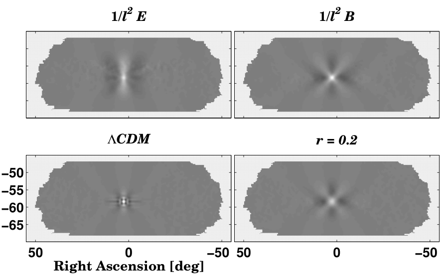
A row of the observed covariance matrix can be reshaped into a map, which reveals the structure of the covariance for a particular pixel, see Figure 13.
VI. separation using a purification matrix
The observed covariance matrix contains expected pixel-pixel covariance in our observed maps given an initial spectrum. The observation matrix, , has made the and -mode spaces of the observed covariance non-orthogonal. The result of Section III is that we can find the orthogonal pure and pure spaces by solving the eigenvalue problem from Equation 19: .
VI.1. Construction of purification matrix
As written, Equation 19 is not solvable: has a null space that is the set of pure -modes. Similarly, the space of pure -modes is the null space of . By adding the identity matrix multiplied by a constant, , to the covariance matrices we regularize the problem to find approximate solutions and eliminate the null spaces:
| (72) |
The amplitude of sets the relative magnitude of the ambiguous mode eigenvalues versus the pure and pure -mode eigenvalues. The eigenvalues are shown in Figure 14. In our analysis, we choose to be 1/100th the mean of the diagonal elements of the covariance matrices, and .
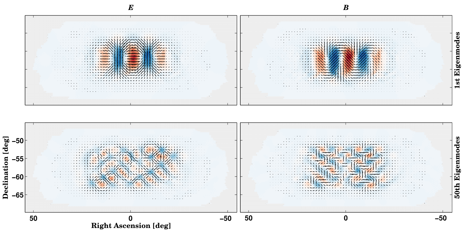
In Equation 72, is an observed covariance matrix for [] that is constructed according to Equations 13 and 71. The input spectrum is set to a steeply red -mode spectrum, , . is the same except for an input spectrum with only -modes, , . The eigenmodes in with the largest eigenvalues comprise a set of vectors that span a space of pure -modes, . The pure quality of these vectors can be seen in the fact that the product is much smaller than the product . The eigenmodes in with the smallest eigenvalues comprise a set of vectors that span a space of pure -modes, .
Using the reddened input spectrum causes the magnitude of the eigenvalues to be proportional to the band of multipole, , that each mode contains. The steepness of the spectrum ensures each mode contains power from a limited range of . The particular choice of is arbitrary.
A basis constructed from a subset of eigenmodes with large eigenvalues spans a subspace of pure -modes. We arbitrarily choose the pure subspace to consist of eigenmodes whose corresponding eigenvalues are the largest of the set. We find modes contained in this subset adequate for preserving power up to 700. The pure subspace is similarly constructed with eigenmodes corresponding to the smallest eigenvalues. Figure 14 shows the sorted eigenvalues, and Figure 15 shows four eigenmodes of the Bicep2 observed covariance.
Using the set of pure and pure -mode basis vectors, two projection matrices are constructed from the outer products:
| (73) |
which we call the purification matrices for pure and pure . Operating the purification matrices on an input map projects onto the space of pure and pure :
| (74) |
From the construction of the pure basis, , one can see that the vector vanishes for arbitrary input containing only -modes: , as desired for a purified map.
VII. Matrix Separation applied to Bicep2
This section describes the application of the matrix based separation to the Bicep2 data set. The technique relies on the existence of the observation matrix and purification matrix from the previous sections.
VII.1. Motivation for matrix based separation in Bicep2
The Bicep2 and Keck Array analysis pipeline contains the following attributes that can leak -modes to -modes: partial sky coverage, timestream filtering (including deprojection), and choice of map projection+estimator. A simulation demonstrating the leaked -mode maps for each of these effects is shown in Figure 16. These maps are created by applying the standard and estimator in Fourier space and then an inversion back to map space. The observations and data reduction produce three classes of leakage:

- •
Apodization: The first obvious deviation from the ideal full sky map is the partial sky coverage of Bicep2 and Keck Array maps. Once a boundary is imposed leakage is created. Map boundary effects are reduced by an apodization window which tapers the maps smoothly to zero near the edges. Use of apodization windows is common practice in any Fourier transform analysis of finite regions to prevent ‘ringing’ near boundaries. For small regions of sky, effects of the map boundary dominate the leakage even after apodization is applied. The apodization window used in Bicep2 and the Keck Array are modified inverse variance maps. We apply a smoothing Gaussian with a width of to the inverse variance map, and, for the combined analyses of Bicep2 and the Keck Array, we use a geometric mean of the individual experiments’ apodization maps.
- •
Map projection: The total extent of the Bicep2 and Keck Array maps is about 50 degrees on the sky in the direction of RA, over a declination of . The chosen projection is a simple rectangular grid of pixels in RA and Dec. Taking standard discrete Fourier transforms of such maps results in significant leakage. While we note that other map projections will have significantly lower distortion, such effects will be present for all projections when subjected to Fourier transform. However, note that the and matrices together fully encode the mapping from the underlying curved sky to the flat sky of the observed map pixels, and therefore so does the observing matrix derived from these.
- •
Linear filtering effects: There are three main analytic filters applied in the standard pipeline: polynomial filter, scan-synchronous subtraction, and deprojection. With respect to to leakage, all three filters are similar: by removing modes in the maps, an -mode can be turned into an observed -mode. Polynomial filtering and scan-synchronous signal subtraction create comparable leakage, both in amplitude and morphology. Deprojection creates more power in the leaked maps, and at smaller angular scales, than either polynomial filtering or scan-synchronous signal subtraction.
If matrix purification is not used, the sample variance of leakage in the Bicep2 power spectrum is comparable to the uncertainty due to instrumental noise. This is clearly highly undesirable, and led to the development of the purification matrix described in this paper. The purification matrix ‘knows about’ all of the mixing effects and how to deal with them.
VII.2. Effectiveness of purification matrix
The effectiveness of the purification matrix given by Equation 74 can be immediately tested by applying the operator to a vector of [] maps simulated with the standard pipeline. The upper left map of Figure 17 shows an observed map whose input is unlensed-CDM -modes, and the next two rows in that column show the resulting and maps after projection onto the pure and spaces. The right column of Figure 17 shows an observed input map with both unlensed-CDM and projected onto pure and -modes.

Matrix purification is integrated with the existing Bicep analysis code by applying the purification operator to maps before calculating the power spectra. Since the observation matrix is only used for this purification step, the purification matrix need only work well enough to result in leakage less than the noise level of the experiment. Therefore, it is acceptable to use an approximate observation matrix constructed from a subset of the full observation list, as long as it is representative of the full scan strategy. This shortcut was employed in Keck Array and Bicep2 Collaborations V [20], but the results shown in this section from Bicep2 are from the full set of observations.
Figure 18 compares the spectra for purified maps to the spectra from maps without purification, and to the spectra found using the improved estimator suggested in Smith [33]. Both the purified maps and unpurified maps use the standard and estimator in Fourier space, and we refer to the unpurified maps processed this way as the ‘normal method.’ Figure 18 shows the spectra for 200 noiseless unlensed-CDM simulations passed through the three estimators. The leaked power is roughly three orders of magnitudes smaller when using the matrix purification than when using the normal method or Smith estimator. While the Smith estimator improves over the normal estimator by eliminating leakage from apodization, it does not account for spatial filtering, which is a significant source of leakage in the analysis pipeline. The mean of the leaked power is de-biased from the final power spectra, so what matters is the variance of the leaked spectra. Computing the 95% confidence limits based on the variance in each of the three methods, we find that in the absence of -mode signal or instrumental noise, the matrix estimator achieves a limit on the tensor-to-scalar ratio of , while the normal method and Smith estimator achieve limits of and respectively.
Figure 19 shows the spectra from the three estimators for input maps containing only input -modes at the level of . The spectra for all three estimators show beam roll off at high . At the lowest , the filtering prevents large angular scale modes from being measured. For multipoles around , the matrix estimator recovers slightly less signal than the other two methods. However, the extra power measured by the other methods near largely comes from the ambiguous modes. On the left of Figure 18, these ambiguous modes are seen as the bump in the normal and Smith method near .
The total number of degrees of freedom in each band power can be estimated according to the formula:
| (75) |
where is the mean of the simulations in band power and is the variance of the simulations in the band power. Table 1 shows the number of degrees of freedom for the three estimators for a tensor -mode. The fewer degrees of freedom at low for the matrix estimator are consistent with the decrease in recovered power on the left side of Figure 18. The highest bins in Table 1 also show fewer degrees of freedom in the matrix estimator because the purification matrix includes a limited number of pure eigenmodes, as shown in Figure 14.
| Degrees of Freedom | |||
|---|---|---|---|
| Bin center, l | Normal | Smith | Matrix |
| 37.5 | 12.9 | 15.5 | 8.6 |
| 72.5 | 40.9 | 41.4 | 34.8 |
| 107.5 | 71.4 | 69.7 | 66.8 |
| 142.5 | 83.7 | 81.2 | 81.7 |
| 177.5 | 120.6 | 116.4 | 116.9 |
| 212.5 | 156.1 | 153.0 | 141.9 |
| 247.5 | 172.0 | 172.9 | 145.8 |
| 282.5 | 202.8 | 200.8 | 177.4 |
| 317.5 | 189.0 | 185.7 | 155.0 |
Figure 20 shows signal plus noise spectra for a set of 200 unlensed-CDM+noise spectra. The noise simulations are the standard Bicep2 sign flip realizations discussed in Bicep2 Collaboration I [4]. In Figure 20, the mean noise level and leaked power are de-biased. The resulting ensemble of simulations is used to construct the errorbars in the final spectra. The tighter distribution of the matrix estimator simulations is a result of the decrease in leakage. Using the matrix estimator results in an improvement in the limit, for Bicep2 noise level and filtering in the absence of -mode signal, of about a factor of two over the Smith method. The remaining variance in the BB spectrum of the matrix estimator is instrumental noise.
VII.3. Transfer functions
The observation matrix transforms an input HEALPix map into an observed map with a simple matrix multiplication. The speed of the operation facilitates the calculation of analysis transfer functions, which are a necessary component of the pseudo- MASTER algorithm [17].
We start with input maps, , which are delta functions in a particular multipole. These maps are then observed using the matrix . The spectra calculated from these maps represent the response in our analysis pipeline to the input delta function, in a manner conceptually analogous to Green’s functions.
Our procedure uses two sets of HEALPix maps, one set corresponding to and one set with . The observation matrix is used to create maps for = through , with 100 random realizations for each . Processing the 140,000 maps would be infeasible without the observation matrix, but using the observation matrix it can be accomplished in a few hours.
VII.3.1 Band power window functions
The power spectra of the output maps for a particular are averaged over the realizations. The averaged spectra are used to form a band power window function, , for a particular band power, , which is a function of the input multipole of the delta function, :
| (76) |
where is the analysis pipeline’s transformation from map to power spectra66 6 Including the steps: apply matrix purification, two dimensional Fourier transform, construction of and , and binning to one dimensional spectra. and . When the input maps contain -modes, and we measure the spectra, the result is the band power window. The use of the purification matrix prevents leakage and makes these band power windows have much lower amplitude than the or ones. In Bicep2, it has been standard procedure not to use the -mode purification matrix, hence the band power window contains (irrelevant) leakage from into .
Calculating the band power window functions in this way accounts for all aspects of our instrument and analysis: beam convolution, sky cut, map projection, polynomial filtering, scan-synchronous signal subtraction, deprojection, and power spectrum estimation.
Figure 21 shows the results of the calculation. Although we bin in annular rings of the two dimensional power spectra, the filtering operations move power from other into those bins. This means the band powers are sensitive to a broader range in than the nominal range of multipoles. The broad shelf in the band power window functions at lower is due to filtering.
Table 2 shows the ‘nominal’ and ‘measured’ centers and edges of the band power bins, where ‘nominal’ refers to the defined range of annular rings in the two dimensional power spectra and ‘measured’ refers to the center and range found in the end to end calculation discussed in this section. The center is the mean of the bandpower window function and the interval corresponds to the percentiles of the bandpower window function between and .
| Nominal | Measured | |||||
|---|---|---|---|---|---|---|
| Bin Number | low | center | high | low | center | high |
| 1 | 20.0 | 37.5 | 55.0 | 37.0 | 46.4 | 54.0 |
| 2 | 55.0 | 72.5 | 90.0 | 59.0 | 73.4 | 86.0 |
| 3 | 90.0 | 107.5 | 125.0 | 92.0 | 107.2 | 121.0 |
| 4 | 125.0 | 142.5 | 160.0 | 125.0 | 140.7 | 157.0 |
| 5 | 160.0 | 177.5 | 195.0 | 158.0 | 173.7 | 192.0 |
| 6 | 195.0 | 212.5 | 230.0 | 189.0 | 205.4 | 227.0 |
| 7 | 230.0 | 247.5 | 265.0 | 220.0 | 237.2 | 262.0 |
| 8 | 265.0 | 282.5 | 300.0 | 253.0 | 270.2 | 298.0 |
| 9 | 300.0 | 317.5 | 335.0 | 285.0 | 302.9 | 333.0 |
Note. — Nominal and measured centers and edges of the band power bins. The measured values are extracted from the band power window functions shown in Figure 21. The low/high values for the latter are the points.
VII.3.2 Suppression factor
The integrated area under the curve of each band power window function represents the response of that band power measurement to an input spectrum. We call this set of values the suppression factor, , since they approximate how our analysis pipeline suppresses power.
The suppression factor is plotted in Figure 22. At small angular scales, the suppression factor is dominated by the roll-off of Bicep2’s 31 arcminute beam. The measured array average 150 GHz beam function is shown as the dotted line in Figure 22. The ‘map window function,’ which includes the finite size of the map and the pixel window function for the degree pixels, is shown as the dashed line77 7 Calculated according to http://healpix.jpl.nasa.gov/html/intronode14.htm. At high , the pixel window function is sub-dominant to the beam window function. At low the suppression factor is dominated by the timestream filtering effects.
VII.4. Computing challenges
Building the observation matrix requires constructing, multiplying, and finally averaging a large number of sparse matrices. Applying the observation matrix to the true sky signal covariance matrix requires a large matrix multiplication to find the product, .
Matrix multiplication is the dominant contributor to computation time. We use matrix multiplication routines built in to MATLAB. These routines incorporate a number of optimized algorithms for computing matrix products, including BLAS [24]. At this time we have not compared the run time on GPUs with that on CPUs, but are aware of this as a possible avenue for reducing the compute time.
Solving the eigenvalue problem using the MATLAB function eig() takes about 48 hrs and 80 GB of RAM for the full Bicep2 observed covariance. For Bicep2, this is small fraction of the total computation time. However, for experiments whose maps contain more pixels, the difficulty of the eigenvalue problem increases. In these cases, the use of distributed memory parallel code may be necessary.
For the Bicep2 results, we used computing resources provided by the Odyssey cluster at Harvard88 8 https://rc.fas.harvard.edu/odyssey/. The Odyssey cluster contains 54K CPUs with 190 terabytes of RAM and 10 petabytes of storage. High memory nodes have access to 256GB of RAM, which is useful for large matrix multiplications. Odyssey uses SLURM99 9 http://slurm.schedmd.com/ as its queue manager, allowing our analysis to utilize the large number of cores available.
Although the raw Bicep2 data set comprises roughly 3 TB of data, the data products from the steps in the matrix analysis chain use 17 TB of storage. Processing during the Bicep2 matrix analysis steps required roughly 1 million CPU hours. This represents a significant portion of the total computing demand of the entire Bicep2 analysis effort, which comprised roughly 6 million CPU hours.
VIII. Conclusions
We have described a method for decomposing an observed polarization field into orthogonal components coming from celestial and -modes. The method relies on numerically calculating an observation matrix. In our case the observation matrix encodes the mathematical steps translating the true sky to an observed map including polynomial filtering, scan-synchronous subtraction, pointing of individual detectors, and linear regression of beam systematics.
Applying the observation matrix to pixel-pixel covariance matrices for and -modes transforms the true sky covariance into the observed space. We then solve for the and eigenmodes and select those modes that are orthogonal. In this way, the orthogonality relationship of the true sky is translated to the observed maps. The method accounts for all types of leakage: boundary effects, polynomial filtering, linear regression, etc.—as long as these properties of the observing strategy and analysis have been encoded in the observation matrix, making the method more general than the method presented in Smith [33], which only accounts for boundary effects.
The observation matrix has many other possibilities and in principle allows construction of fully optimal analyses through to power spectra or cosmological parameters for a single experiment, or a combination of experiments with partially overlapping sky coverage. One simple application which we have explored is to use the observation matrix to directly produce simulated observed maps from input maps in a single step. This is dramatically faster than the previous standard pipeline. However production of observing matrices is sufficiently costly that we have not generated them for the many alternate “jackknife” data split maps and so for the present standard simulations are still required.
We find that the matrix based separation performs quite well, limiting the leakage to a level corresponding to , well below the noise level for any foreseeable CMB experiment. The method should prove useful for future ground based or balloon based experiments focused on measuring large angular scale -modes. Experiments measuring the lensing potential using CMB polarization rely on cleanly separating and as well and may find the technique useful. Additionally, the ongoing search for the imprint of gravitational waves in CMB polarization will require mitigation of lensing signal from intervening structure and foreground removal, both of which are improved by cleanly separating and .
Appendix A Generation of constrained realization HEALPix maps
An ensemble of signal only simulations is needed for a MASTER pseudo- analysis. We use CAMB with input Planck parameters to construct power spectra, . The power spectra are used to generate high resolution HEALPix maps that serve as the starting point for each realization of the signal simulations. Lacking any constraints on the realizations, the maps generated from the power spectra will vary for both the temperature and polarization fields. However, Planck has measured the temperature field of the CMB to high signal to noise. Since the goal of Bicep2 and the Keck Array is to measure the polarization sky and not the temperature sky, our ensemble of simulations does not need to contain variation in the well measured temperature sky. We therefore use the temperature field of the CMB measured by Planck as the template for constrained realizations of the polarization field.
We have developed a technique for creating realizations of the -mode sky consistent with the known correlation and the measured temperature field. These constrained realizations have been shown to contain the same correlations and spectra over many realizations of the temperature sky. However, any particular set of constrained realizations based on one temperature sky has a slightly different distribution of and than the full ensemble average.
The primary motivation for fixing the temperature field is to make the deprojection operation discussed in Section IV.10 into a linear operator. Recall that deprojection involves a regression against a fixed template of the temperature sky. If the temperature sky varies from realization to realization, deprojection becomes non-linear and cannot be expressed as a matrix operation.
A.1. correlation
We start by fixing the coefficients of the spherical harmonics of the temperature sky, . The for the constrained -modes is found in Dvorkin et al. [11] and can be derived following the steps of a simple Cholesky decomposition. The covariance between and for each mode () is:
| (A1) |
The lower triangle Cholesky decomposition of this matrix determines the variance and covariance in each mode:
| (A2) |
where and are unit norm, complex random numbers. Since are known constraints, we can solve the system of equations:
| (A3) |
substituting the first equation into the second to arrive at an expression for in terms of and the power spectra, . To ensure the maps are real, the condition is demanded.
Naively, we might expect the constrained to have lower variance in its power spectrum than the unconstrained since there is significant correlation and the temperature component is fixed. However, this is not necessarily the case. When the fluctuate high, the mean of the constrained ensemble of ’s is also high, resulting in increased variance in the ensemble of simulations. For particularly high , this can result in larger variance for the constrained simulations than the unconstrained simulations. This happens to be the case in the Bicep field near , as seen in Figure 23.
In practice, we take the from the Planck temperature Needlet Internal Linear Combination (NILC) map [27]. This map uses the multi-frequency coverage of Planck to remove the galactic contribution to microwave emission, leaving a high signal to noise map of the CMB temperature field. The map has some contamination near the galactic plane. However, we have found that the impact of this is very local and does not affect the higher galactic latitudes where the Bicep field is located. The noise level in the Planck temperature map is fractionally small compared to the temperature signal, and we have found that this noise contributes a similarly small fraction to the constrained realization of -modes.
A.2. Lensing
The temperature anisotropies in the Planck NILC map have been lensed by the intervening structure between us and the surface of last scattering. This means the calculated from the Planck NILC map contain the effects of lensing and when used in Equation A3, the lensing distortion propagates through to the constrained . Ideally, the in Equation A3 would be from the unlensed sky, however, in the absence of an accurate map of the lensing deflection field, we have no way of de-lensing the .
Because our power spectrum analysis is insensitive to the off-diagonal correlations among modes with that are produced by lensing, a reasonable workaround for this problem is to use the Planck NILC but also to use the lensed spectrum. The result is an ensemble of for the lensed , but which have the correct covariance given by . For the multipole range of interest in Bicep2, lensing has a small impact on . We use the unlensed power spectra for and .
Another subtlety incorporating lensing into constrained realizations is the question of how to simulate lensing of the polarization sky. This can be accomplished using LensPix [25] to numerically lens the primordial -modes, which creates -modes with the correct statistics. For the constrained realizations, this is impossible because the NILC map is lensed by the true sky lensing field. The true sky lensing field is not known with high signal to noise, and therefore we cannot lens the -modes by the same field.
Our solution to this problem is to lens the -modes with a random realization of the lensing field, but use the Planck 143 GHz map as the temperature field. This procedure ignores lensing correlations in and because the deflection field is different for the polarization and temperature. However, the mean of the lensing and is zero, and the additional variance in and caused by lensing is small enough that it can be ignored on degree scales.
References
- [1] Aikin, R. W. 2013, PhD thesis, California Institute of Technology
- [2] Bicep1 Collaboration. 2014, Astrophys. J., 783, 67
- [3] Bicep2/Keck and Spider Collaborations. 2015, Astrophys. J., 812, 176
- [4] Bicep2 Collaboration I. 2014, Physical Review Letters, 112, 241101
- [5] Bicep2 Collaboration II. 2014, Astrophys. J., 792, 62
- [6] Bicep2 Collaboration III. 2015, Astrophys. J., 814, 110
- [7] Bischoff, C., Hyatt, L., McMahon, J. J., et al. 2008, Astrophys. J., 684, 771
- [8] Bond, J., Jaffe, A. H., & Knox, L. 1998, Phys.Rev., D57, 2117
- [9] Bunn, E. F., & White, M. 1997, The Astrophysical Journal, 480, 6
- [10] Bunn, E. F., Zaldarriaga, M., Tegmark, M., & Oliveira-Costa, A. d. 2003, Phys.Rev., D67, 023501
- [11] Dvorkin, C., Peiris, H. V., & Hu, W. 2008, Phys.Rev., D77, 063008
- [12] Goldberg, J. N., Macfarlane, A. J., Newman, E. T., Rohrlich, F., & Sudarshan, E. C. G. 1967, Journal of Mathematical Physics, 8, 2155
- [13] Gorski, K., Hivon, E., Banday, A., et al. 2005, Astrophys.J., 622, 759
- [14] Grain, J., Tristram, M., & Stompor, R. 2009, Phys. Rev. D, 79, 123515
- [15] Hamaker, J. P., & Bregman, J. D. 1996, aaps, 117, 161
- [16] Hanson, D., Hoover, S., Crites, A., et al. 2013, Physical Review Letters, 111, 141301
- [17] Hivon, E., Górski, K. M., Netterfield, C. B., et al. 2002, Astrophys. J., 567, 2
- [18] Hu, W., Hedman, M. M., & Zaldarriaga, M. 2003, Phys. Rev. D, 67, 043004
- [19] Kamionkowski, M., Kosowsky, A., & Stebbins, A. 1997, Phys.Rev., D55, 7368
- [20] Keck Array and Bicep2 Collaborations V. 2015, Astrophys. J., 811, 126
- [21] Keck Array and Bicep2 Collaborations VI. 2016, Physical Review Letters, 116, 031302
- [22] Kovac, J. M., Leitch, E. M., Pryke, C., et al. 2002, Nature, 420, 772
- [23] Kuo, C., Ade, P., Bock, J., et al. 2004, Astrophys.J., 600, 32
- [24] Lawson, C. L., Hanson, R. J., Kincaid, D. R., & Krogh, F. T. 1979, ACM Trans. Math. Softw., 5, 308
- [25] Lewis, A. 2011, LensPix: Fast MPI full sky transforms for HEALPix, astrophysics Source Code Library, ascl:1102.025
- [26] Planck Collaboration I. 2015, ArXiv e-prints, arXiv:1502.01582
- [27] Planck Collaboration XII. 2014, Astr. & Astroph., 571, A12
- [28] Polarbear Collaboration. 2014, Astrophys. J., 794, 171
- [29] Pryke, C., Ade, P., Bock, J., et al. 2009, Astrophys. J., 692, 1247
- [30] Readhead, A. C. S., Myers, S. T., Pearson, T. J., et al. 2004, Science, 306, 836
- [31] Sheehy, C. D. 2013, PhD thesis, University of Chicago, copyright - Copyright ProQuest, UMI Dissertations Publishing 2013; Last updated - 2014-02-11; First page - n/a; M3: Ph.D.
- [32] Shimon, M., Keating, B., Ponthieu, N., & Hivon, E. 2008, Phys. Rev. D, 77, 083003
- [33] Smith, K. M. 2006, Phys. Rev. D, 74, 083002
- [34] Smith, K. M., & Zaldarriaga, M. 2007, Phys.Rev., D76, 043001
- [35] Tegmark, M. 1997, Phys. Rev. D, 55, 5895
- [36] Tegmark, M., & de Oliveira-Costa, A. 2001, Phys. Rev. D, 64, 063001
- [37] van Engelen, A., Sherwin, B. D., Sehgal, N., et al. 2015, Astrophys. J., 808, 7
- [38] Zaldarriaga, M. 1998, The Astrophysical Journal, 503, 1
- [39] Zaldarriaga, M., & Seljak, U. 1997, Phys.Rev., D55, 1830