跳到论文正文
W Papers独立论文阅读器 arXiv:1603.05948 论文正文 计算阅读时间 · 0%
引用这篇论文根据当前论文元数据生成,正式投稿前建议核对。


License: arXiv.org perpetual non-exclusive license
arXiv:1603.05948v1 [math.NT] 18 Mar 2016

Evaluating Generating Functions for Periodic Multiple Polylogarithms via Rational Chen–Fliess Series

Kurusch Ebrahimi-Fard Address: ICMAT, C/ Nicolás Cabrera, no. 13-15, 28049 Madrid, Spain On leave from UHA, Mulhouse, France. Email address: kurusch@icmat.es URL: http://www.icmat.es/kurusch/personal , W. Steven Gray Address: Old Dominion University, Norfolk, Virginia, 23454, U.S.A. Email address: sgray@odu.edu and Dominique Manchon Address: Université Blaise Pascal, C.N.R.S.-UMR 6620, BP 80026, 63171 Aubière, France Email address: manchon@math.univ-bpclermont.fr URL: http://math.univ-bpclermont.fr/˜manchon/
Date: August 24, 2026
Abstract.

The goal of the paper is to give a systematic way to numerically evaluate the generating function of a periodic multiple polylogarithm using a Chen–Fliess series with a rational generating series. The idea is to realize the corresponding Chen–Fliess series as a bilinear dynamical system. A standard form for such a realization is given. The method is also generalized to the case where the multiple polylogarithm has non-periodic components. This allows one, for instance, to numerically validate the Hoffman conjecture. Finally, a setting in terms of dendriform algebras is provided.

Keywords: multiple polylogarithms, multiple zeta values, Chen–Fliess series, rational formal power series

Math. Subject Classification: 11G55, 11M32, 93B20, 93C10.

1. Introduction

Given any vector 𝐬=(s1,s2,…,sl)∈ℤl\mathbf{s}=(s_{1},s_{2},\ldots,s_{l})\in\mathbb{Z}^{l} with s1≥2s_{1}\geq 2 and si≥1s_{i}\geq 1 for i≥2i\geq 2, the associated multiple polylogarithm (MPL) of depth ll and weight |𝐬|:=∑i=1lsi\left|\mathbf{s}\right|:=\sum_{i=1}^{l}s_{i} is taken to be

(1) Li𝐬​(t):=∑k1>k2>⋯>kl≥1tk1k1s1k2s2⋯klsl,|t|≤1,\mathrm{Li}_{\mathbf{s}}(t):=\sum_{k_{1}>k_{2}>\cdots>k_{l}\geq 1}\frac{t^{k_{1}}}{k_{1}^{s_{1}}k_{2}^{s_{2}}\cdots k_{l}^{s_{l}}},\quad\left|t\right|\leq 1,

whereupon the multiple zeta value (MVZ) of depth ll and weight |𝐬|\left|\mathbf{s}\right| is the value of (1) at t=1t=1, namely,

ζ​(𝐬):=Li𝐬​(1).\zeta(\mathbf{s}):=\mathrm{Li}_{\mathbf{s}}(1).

Any such vector 𝐬\mathbf{s} will be referred to as admissible. The MPL in (1) can be represented in terms of iterated Chen integrals with respect to the 11-forms ωj(1):=d​tj1−tj\omega_{j}^{(1)}:=\frac{dt_{j}}{1-t_{j}} and ωj(0):=d​tjtj\omega_{j}^{(0)}:=\frac{dt_{j}}{t_{j}}. Indeed, using the standard notation, |𝐬(j)|:=s1+⋯+sj|\mathbf{s}_{(j)}|:=s_{1}+\cdots+s_{j}, j∈{1,…,l}j\in\{1,\ldots,l\}, one can show that

(2) Li𝐬(t)=∫0t(∏j=1|𝐬(1)|−1ωj(0))ω|𝐬(1)|(1)⋯(∏j=|𝐬(l−1)|+1|𝐬(l)|−1ωj(0))ω|𝐬(l)|(1).\mathrm{Li}_{\mathbf{s}}(t)=\int_{0}^{t}\bigg(\prod_{j=1}^{|\mathbf{s}_{(1)}|-1}\omega_{j}^{(0)}\bigg)\omega_{|\mathbf{s}_{(1)}|}^{(1)}\cdots\bigg(\prod_{j=|\mathbf{s}_{(l-1)}|+1}^{|\mathbf{s}_{(l)}|-1}\omega_{j}^{(0)}\bigg)\omega_{|\mathbf{s}_{(l)}|}^{(1)}.

For instance,

Li(2,1,1)​(t)\displaystyle\mathrm{Li}_{(2,1,1)}(t) =∫0td​t1t1​∫0t1d​t21−t2​∫0t2d​t31−t3​∫0t3d​t41−t4=∑k1>k2>k3≥1tk1k12​k2​k3.\displaystyle=\int_{0}^{t}\frac{dt_{1}}{t_{1}}\int_{0}^{t_{1}}\frac{dt_{2}}{1-t_{2}}\int_{0}^{t_{2}}\frac{dt_{3}}{1-t_{3}}\int_{0}^{t_{3}}\frac{dt_{4}}{1-t_{4}}=\sum_{k_{1}>k_{2}>k_{3}\geq 1}\frac{t^{k_{1}}}{k_{1}^{2}k_{2}k_{3}}.

An MPL of depth ll is said to be periodic if it can be written in the form Li{𝐬}n​(t)\mathrm{Li}_{\mathbf{\{s\}}^{n}}(t), where {𝐬}n\{\mathbf{s}\}^{n} denotes the nn-tuple (𝐬,𝐬,…,𝐬)∈ℤn​l(\mathbf{s},\mathbf{s},\ldots,\mathbf{s})\in\mathbb{Z}^{nl}, n≥0n\geq 0 with Li{𝐬}0​(t):=1\mathrm{Li}_{\{\mathbf{s}\}^{0}}(t):=1.11 1 Following other authors, {𝐬}n={(s1,s2,…,sl)}n\{\mathbf{s}\}^{n}=\{(s_{1},s_{2},\ldots,s_{l})\}^{n} will be written more concisely as {s1,s2,…,sl}n\{s_{1},s_{2},\ldots,s_{l}\}^{n}. In this case, the sequence (Li{𝐬}n​(t))n∈ℕ0(\mathrm{Li}_{\{\mathbf{s}\}^{n}}(t))_{n\in\mathbb{N}_{0}} has the generating function

(3) ℒ𝐬​(t,θ):=∑n=0∞Li{𝐬}n​(t)​(θ|𝐬|)n.\mathcal{L}_{\bf s}(t,\theta):=\sum_{n=0}^{\infty}\mathrm{Li}_{\{\mathbf{s}\}^{n}}(t)\left(\theta^{\left|\mathbf{s}\right|}\right)^{n}.

In general, the integral representation (2) implies that ℒ𝐬\mathcal{L}_{\mathbf{s}} will satisfy a linear ordinary differential equation in tt whose solution can be written in terms of a hypergeometric function [1, 4, 5, 21, 22, 23, 24]. For example, when l=1l=1 and 𝐬=(s)\mathbf{s}=(s), it follows that

(4) (((1−t)​dd​t)​(t​dd​t)s−1−θs)​ℒ𝐬​(t,θ)=0,\left(\left((1-t)\frac{d}{dt}\right)\left(t\frac{d}{dt}\right)^{s-1}-\theta^{s}\right)\mathcal{L}_{\mathbf{s}}(t,\theta)=0,

and its solution is the Euler–Gauss hypergeometric function

ℒ(s)(t,θ)=sFs−1(−ω​θ,−ω3​θ,…,−ω2​s−1​θ1,1,…,1|t),\mathcal{L}_{(s)}(t,\theta)=_{s}\!F_{s-1}\left(\left.\begin{array}[]{c}-\omega\theta,-\omega^{3}\theta,\ldots,-\omega^{2s-1}\theta\\ 1,1,\ldots,1\end{array}\right|t\right),

where ω=eπ​i/s\omega={\rm e}^{\pi i/s}, a primitive ss-th root of −1-1 [4]. By expanding this solution into a hypergeometric series and equating like powers of θ\theta with those in (3), it is possible to show, for example, when s=2s=2 that

(5) ζ⁡({2}n)=π2​n(2​n+1)!,n≥1.\zeta(\{2\}^{n})=\frac{\pi^{2n}}{(2n+1)!},\quad n\geq 1.

In a similar manner it can be shown that

ζ⁡({3,1}n)=2​π4​n(4​n+2)!,n≥1.\zeta(\{3,1\}^{n})=\frac{2\pi^{4n}}{(4n+2)!},\quad n\geq 1.

This method has yielded a plethora of such MZV identities [3, 4, 6, 25]. The most general case is treated in [24], where it is shown that ℒ𝐬\mathcal{L}_{\mathbf{s}} satisfies the linear differential equation of Fuchs type

(6) (P𝐬−θ|𝐬|)​ℒ𝐬​(t,θ)=0,(P_{\mathbf{s}}-\theta^{\left|\mathbf{s}\right|})\mathcal{L}_{\mathbf{s}}(t,\theta)=0,

where for 𝐬=(s1,s2,…,sl)∈ℤl\mathbf{s}=(s_{1},s_{2},\ldots,s_{l})\in\mathbb{Z}^{l}

P𝐬:=PslPsl−1⋯Ps1P_{\mathbf{s}}:=P_{s_{l}}P_{s_{l-1}}\cdots P_{s_{1}}

and

Psi:=((1−t)​dd​t)​(t​dd​t)si−1.P_{s_{i}}:=\left((1-t)\frac{d}{dt}\right)\left(t\frac{d}{dt}\right)^{s_{i}-1}.

(The conventions in [24] are to use −θ-\theta in place of θ\theta and tt in place of 1−t1-t.) In [24] and related work [21, 22, 23], the authors develop WKB type asymptotic expansions of these hypergeometric solutions.

The ultimate goal of the present paper is to provide a numerical scheme for estimating ℒ𝐬​(t,θ)\mathcal{L}_{\bf s}(t,\theta) by in essence mapping the |𝐬|\left|{\bf s}\right|-order linear differential equation (6) to a system of |𝐬|\left|{\bf s}\right| first-order bilinear differential equations which can be solved by standard tools found in software packages like MatLab. Specifically, it will be shown how to construct a dynamical system of the form

(7a) z˙\displaystyle\dot{z} =N0​z​u0+N1​z​u1,z⁡(0)=z0\displaystyle=N_{0}z\,u_{0}+N_{1}z\,u_{1},\;\;z(0)=z_{0}
(7b) y\displaystyle y =C​z,\displaystyle=Cz,

which when simulated over the interval [0,1][0,1] has the property that y⁡(t)=ℒ𝐬​(t,θ)y(t)=\mathcal{L}_{\mathbf{s}}(t,\theta) for any value of θ\theta and t∈[0,1]t\in[0,1]. In this case, the matrices N0N_{0} and N1N_{1} will depend on θ\theta, and the initial condition z0z_{0} and the input functions u0u_{0}, u1u_{1} must be suitably chosen. Such a technique could be useful for either disproving certain conjectures involving MZVs or providing additional evidence for the truthfulness of other conjectures. For example, one could validate with a certain level of (numerical) confidence a conjecture of the form

ζ⁡({𝐬a}n)=bn​ζ​({𝐬b}n),n∈ℕ,b∈ℤ,\zeta(\{\mathbf{s}_{a}\}^{n})=b^{n}\zeta(\{\mathbf{s}_{b}\}^{n}),\quad n\in\mathbb{N},b\in\mathbb{Z},

where 𝐬a∈ℤla\mathbf{s}_{a}\in\mathbb{Z}^{l_{a}}, 𝐬b∈ℤlb\mathbf{s}_{b}\in\mathbb{Z}^{l_{b}} with |𝐬a|=|𝐬b|\left|\mathbf{s}_{a}\right|=\left|\mathbf{s}_{b}\right|. Take as a specific example the known identity

(8) ζ⁡({4}n)=4n​ζ​({3,1}n)\zeta(\{4\}^{n})=4^{n}\zeta(\{3,1\}^{n})

for all n≥1n\geq 1, so that 𝐬a=(4)\mathbf{s}_{a}=(4), 𝐬b=(3,1)\mathbf{s}_{b}=(3,1) and b=4b=4 [4]. Note that for n=1n=1 the identity follows immediately from double shuffle relations for MZVs [18]. On the level of generating functions it is evident that

ℒ(4)​(1,θ)\displaystyle\mathcal{L}_{(4)}(1,\theta) =∑n=0∞Li{4}n​(1)​(θ4)n=∑n=0∞ζ⁡({4}n)​θ4​n\displaystyle=\sum_{n=0}^{\infty}\mathrm{Li}_{\{4\}^{n}}(1)\left(\theta^{4}\right)^{n}=\sum_{n=0}^{\infty}\zeta(\{4\}^{n})\,\theta^{4n}
ℒ(3,1)​(1,2​θ)\displaystyle\mathcal{L}_{(3,1)}(1,\sqrt{2}\theta) =∑n=0∞Li{3,1}n​(1)​((2​θ)4)n=∑n=0∞4n​ζ​({3,1}n)​θ4​n.\displaystyle=\sum_{n=0}^{\infty}\mathrm{Li}_{\{3,1\}^{n}}(1)\left((\sqrt{2}\theta)^{4}\right)^{n}=\sum_{n=0}^{\infty}4^{n}\zeta(\{3,1\}^{n})\,\theta^{4n}.

Therefore, identity (8) implies that

(9) ℒ(4)​(1,θ)−ℒ(3,1)​(1,2​θ)=0,∀θ∈ℝ,\mathcal{L}_{(4)}(1,\theta)-\mathcal{L}_{(3,1)}(1,\sqrt{2}\theta)=0,\quad\forall\theta\in{\mathbb{R}},

a claim that can be tested empirically if these generating functions can be accurately evaluated. The method can also be generalized to address the conjecture of Hoffman that

(10) ζ⁡({2}n,2,2,2)+2​ζ​({2}n,3,3)=ζ⁡(2,1,{2}n,3),\zeta(\{2\}^{n},2,2,2)+2\zeta(\{2\}^{n},3,3)=\zeta(2,1,\{2\}^{n},3),

for all integers n>0n>0, which has only been proved for n≤8n\leq 8 [6]. The idea here is to admit non-periodic components in the generating function calculation. For example, ({2}n,3,3)(\{2\}^{n},3,3) can be viewed as having the periodic component {2}n\{2\}^{n} and the non-periodic component (3,3)(3,3). In the general case, say when 𝒔n:=(𝐬a,{𝐬b}n,𝐬c)\hbox{$s$}_{n}:=(\mathbf{s}_{a},\{\mathbf{s}_{b}\}^{n},\mathbf{s}_{c}), n≥0n\geq 0, the generating function is defined analogously as

ℒ(𝐬a,{𝐬b},𝐬c)​(t,θ):=∑n=0∞Li𝐬n​(t)​(θ|𝐬b|)n.\mathcal{L}_{(\mathbf{s}_{a},\{\mathbf{s}_{b}\},\mathbf{s}_{c})}(t,\theta):=\sum_{n=0}^{\infty}{\rm Li}_{{\mathbf{s}}_{n}}(t)\left(\theta^{\left|\mathbf{s}_{b}\right|}\right)^{n}.

Therefore, relation (10), if true, would imply that

(11) ℒ({2},2,2,2)​(1,θ)+2​ℒ({2},3,3)​(1,θ)−ℒ(2,1,{2},3)​(1,θ)=0,∀θ∈ℝ.\mathcal{L}_{(\{2\},2,2,2)}(1,\theta)+2\mathcal{L}_{(\{2\},3,3)}(1,\theta)-\mathcal{L}_{(2,1,\{2\},3)}(1,\theta)=0,\quad\forall\theta\in{\mathbb{R}}.

The basic approach to estimating ℒ𝐬​(t,θ)\mathcal{L}_{\bf s}(t,\theta) is to map a periodic multiple polylogarithm to a rational series and then to employ concepts from control theory to produce bilinear state space realization (7) of the corresponding rational Chen–Fliess series [2, 14, 15]. The periodic nature of the MPL always ensures that these realizations have a certain built-in recursion/feedback structure. The technique will first be described in general, and then it will be demonstrated by empirically verifying the identities (5), (8), and (10).

The paper is organized as follows. In the next section, a brief summary of rational Chen–Fliess series is given to establish the notation and the basic concepts to be employed. Then the general method for evaluating a generating function of a periodic multiple polylogarithm is given in the subsequent section, which also contains in Subsection 3.3 a short digression regarding another way of looking at periodic MPLs in terms of the shuffle algebra. This is followed by several examples in Section 4. In particular, the last example shows that the Hoffman conjecture (10) has a high likelihood of being true. The final section gives the paper’s conclusions.

2. Preliminaries

2.1. Chen–Fliess series

A finite nonempty set of noncommuting symbols X={x0,x1,X=\{x_{0},x_{1}, …,xm}\ldots,x_{m}\} is called an alphabet. Each element of XX is called a letter, and any finite sequence of letters from XX, η=xi1⋯xik\eta=x_{i_{1}}\cdots x_{i_{k}}, is called a word over XX. The length of word η\eta, denoted |η|\left|\eta\right|, is the number of letters in η\eta. The set of all words with fixed length kk is denoted by XkX^{k}. The set of all words including the empty word, ∅\emptyset, is designated by X∗X^{\ast}. It forms a monoid under catenation. The set η​X∗​ξ⊆X∗\eta X^{\ast}\xi\subseteq X^{\ast} is the set of all words with prefix η\eta and suffix ξ\xi. Any mapping c:X∗→ℝℓc:X^{\ast}\rightarrow{\mathbb{R}}^{\ell} is called a formal power series. The value of cc at η∈X∗\eta\in X^{\ast} is written as (c,η)∈ℝℓ(c,\eta)\in{\mathbb{R}}^{\ell} and called the coefficient of the word η\eta in the series cc. Typically, cc is represented as the formal sum c=∑η∈X∗(c,η)​η.c=\sum_{\eta\in X^{\ast}}(c,\eta)\eta. If the constant term (c,∅)=0(c,\emptyset)=0 then cc is said to be proper. The collection of all formal power series over the alphabet XX is denoted by ℝℓ​⟨⟨X⟩⟩{\mathbb{R}}^{\ell}\langle\langle X\rangle\rangle. The subset of polynomials is written as ℝℓ​⟨X⟩{\mathbb{R}}^{\ell}\langle X\rangle. Each set forms an associative ℝ{\mathbb{R}}-algebra under the catenation product.

Definition 1.

Given ξ∈X∗\xi\in X^{\ast}, the corresponding left-shift operator ξ−1:X∗→X∗\xi^{-1}:X^{\ast}\rightarrow X^{\ast} is defined:

η↦ξ−1(η):={η′:η=ξ​η′0:otherwise.\eta\mapsto\xi^{-1}(\eta):=\left\{\begin{array}[]{ccl}\eta^{\prime}&:&\eta=\xi\eta^{\prime}\\[2.168pt] 0&:&\hbox{otherwise}.\end{array}\right.

It is extended linearly to ℝℓ​⟨⟨X⟩⟩{\mathbb{R}}^{\ell}\langle\langle X\rangle\rangle.

One can formally associate with any series c∈ℝℓ​⟨⟨X⟩⟩c\in\mbox{${\mathbb{R}}^{\ell}\langle\langle X\rangle\rangle$} a causal mm-input, ℓ\ell-output operator, FcF_{c}, in the following manner. Let 𝔭≥1\mathfrak{p}\geq 1 and t0<t1t_{0}<t_{1} be given. For a Lebesgue measurable function u:[t0,t1]→ℝmu:[t_{0},t_{1}]\rightarrow{\mathbb{R}}^{m}, define ‖u‖𝔭:=max⁡{‖ui‖𝔭: 1≤i≤m}\left\|u\right\|_{\mathfrak{p}}:=\max\{\left\|u_{i}\right\|_{\mathfrak{p}}:\ 1\leq i\leq m\}, where ‖ui‖𝔭\left\|u_{i}\right\|_{\mathfrak{p}} is the usual L𝔭L_{\mathfrak{p}}-norm for a measurable real-valued function, uiu_{i}, defined on the interval [t0,t1][t_{0},t_{1}]. Let L𝔭m​[t0,t1]L^{m}_{\mathfrak{p}}[t_{0},t_{1}] denote the set of all measurable functions defined on [t0,t1][t_{0},t_{1}] having a finite ‖⋅‖𝔭\left\|\cdot\right\|_{\mathfrak{p}} norm and B𝔭m​(R)​[t0,t1]:={u∈L𝔭m​[t0,t1]:‖u‖𝔭≤R}B_{\mathfrak{p}}^{m}(R)[t_{0},t_{1}]:=\{u\in L_{\mathfrak{p}}^{m}[t_{0},t_{1}]:\left\|u\right\|_{\mathfrak{p}}\leq R\}. Assume C⁡[t0,t1]C[t_{0},t_{1}] is the subset of continuous functions in L1m​[t0,t1]L_{1}^{m}[t_{0},t_{1}]. Define inductively for each word η∈X∗\eta\in X^{\ast} the map Eη:L1m​[t0,t1]→C⁡[t0,t1]E_{\eta}:L_{1}^{m}[t_{0},t_{1}]\rightarrow C[t_{0},t_{1}] by setting E∅​[u]=1E_{\emptyset}[u]=1 and letting

Exi​η¯​[u]​(t,t0):=∫t0tui​(τ)​Eη¯​[u]​(τ,t0)​𝑑τ,E_{x_{i}\bar{\eta}}[u](t,t_{0}):=\int_{t_{0}}^{t}u_{i}(\tau)E_{\bar{\eta}}[u](\tau,t_{0})\,d\tau,

where xi∈Xx_{i}\in X, η¯∈X∗\bar{\eta}\in X^{\ast}, and u0=1u_{0}=1. The input-output operator corresponding to the series c∈ℝℓ​⟨⟨X⟩⟩c\in\mbox{${\mathbb{R}}^{\ell}\langle\langle X\rangle\rangle$} is the Fliess operator or Chen–Fliess series

(12) Fc​[u]​(t)=∑η∈X∗(c,η)​Eη​[u]​(t,t0).F_{c}[u](t)=\sum_{\eta\in X^{\ast}}(c,\eta)\,E_{\eta}[u](t,t_{0}).

If there exist real numbers Kc,Mc>0K_{c},M_{c}>0 and r∈[0,1)r\in[0,1) such that the coefficients of the generating series c=∑η∈X∗(c,η)​η∈ℝℓ​⟨⟨X⟩⟩c=\sum_{\eta\in X^{\ast}}(c,\eta)\eta\in\mbox{${\mathbb{R}}^{\ell}\langle\langle X\rangle\rangle$} satisfying the growth bound

(13) |(c,η)|≤Kc​Mc|η|​(|η|!)r,∀η∈X∗,\left|(c,\eta)\right|\leq K_{c}M_{c}^{|\eta|}(\left|\eta\right|!)^{r},\quad\forall\eta\in X^{\ast},

then the series (12) defines an operator from the extended space L𝔭,em​(t0)L^{m}_{\mathfrak{p},e}(t_{0}) into C[t0,∞)C[t_{0},\infty), where

L𝔭,em(t0):={u:[t0,∞)→ℝm:u[t0,t1]∈L𝔭m[t0,t1],∀t1∈(t0,∞)},L^{m}_{\mathfrak{p},e}(t_{0}):=\{u:[t_{0},\infty)\rightarrow{\mathbb{R}}^{m}:u_{[t_{0},t_{1}]}\in L_{\mathfrak{p}}^{m}[t_{0},t_{1}],\;\forall t_{1}\in(t_{0},\infty)\},

and u[t0,t1]u_{[t_{0},t_{1}]} denotes the restriction of uu to the intervall [t0,t1][t_{0},t_{1}]. (Here, |z|:=maxi⁡|zi|\left|z\right|:=\max_{i}\left|z_{i}\right| when z∈ℝℓz\in{\mathbb{R}}^{\ell}.) See [20] for details. In this case, the operator is said to be globally convergent, and the set of all series satisfying (13) is designated by ℝG​Cℓ​⟨⟨X⟩⟩{\mathbb{R}}^{\ell}_{GC}\langle\langle X\rangle\rangle. In the following sections, it suffices to set ℓ=m=1\ell=m=1, which corresponds to the single-input, single-output (SISO) case.

2.2. Bilinear realizations of rational Chen–Fliess series

A series c∈ℝ​⟨⟨X⟩⟩c\in\mbox{${\mathbb{R}}\langle\langle X\rangle\rangle$} is called invertible if there exists a series c−1∈ℝ​⟨⟨X⟩⟩c^{-1}\in\mbox{${\mathbb{R}}\langle\langle X\rangle\rangle$} such that c​c−1=c−1​c=1cc^{-1}=c^{-1}c=1.22 2 The polynomial 1​∅1\emptyset is abbreviated throughout as 11. In the event that cc is not proper, i.e., the coefficient (c,∅)(c,\emptyset) is nonzero, it is always possible to write

c=(c,∅)​(1−c′),c=(c,\emptyset)(1-c^{\prime}),

where c′∈ℝ​⟨⟨X⟩⟩c^{\prime}\in\mbox{${\mathbb{R}}\langle\langle X\rangle\rangle$} is proper. It then follows that

c−1=1(c,∅)​(1−c′)−1=1(c,∅)​(c′)∗,c^{-1}=\frac{1}{(c,\emptyset)}(1-c^{\prime})^{-1}=\frac{1}{(c,\emptyset)}(c^{\prime})^{\ast},

where

(c′)∗:=∑i=0∞(c′)i.(c^{\prime})^{\ast}:=\sum_{i=0}^{\infty}(c^{\prime})^{i}.

In fact, c∈ℝ​⟨⟨X⟩⟩c\in\mbox{${\mathbb{R}}\langle\langle X\rangle\rangle$} is invertible if and only if cc is not proper. Now let SS be a subalgebra of the ℝ{\mathbb{R}}-algebra ℝ​⟨⟨X⟩⟩{\mathbb{R}}\langle\langle X\rangle\rangle with the catenation product. SS is said to be rationally closed when every invertible c∈Sc\in S has c−1∈Sc^{-1}\in S (or equivalently, every proper c′∈Sc^{\prime}\in S has (c′)∗∈S(c^{\prime})^{\ast}\in S). The rational closure of any subset E⊂ℝ​⟨⟨X⟩⟩E\subset\mbox{${\mathbb{R}}\langle\langle X\rangle\rangle$} is the smallest rationally closed subalgebra of ℝ​⟨⟨X⟩⟩{\mathbb{R}}\langle\langle X\rangle\rangle containing EE.

Definition 2.

A series c∈ℝ​⟨⟨X⟩⟩c\in\mbox{${\mathbb{R}}\langle\langle X\rangle\rangle$} is rational if it belongs to the rational closure of ℝ​⟨X⟩{\mathbb{R}}\langle X\rangle.

It turns out that an entirely different characterization of a rational series is possible using the following concept.

Definition 3.

A linear representation of a series c∈ℝ​⟨⟨X⟩⟩c\in\mbox{${\mathbb{R}}\langle\langle X\rangle\rangle$} is any triple (μ,γ,λ)(\mu,\gamma,\lambda), where

μ:X∗→ℝn×n\mu:X^{\ast}\rightarrow{\mathbb{R}}^{n\times n}

is a monoid morphism, and the vectors γ,λT∈ℝn×1\gamma,\lambda^{T}\in{\mathbb{R}}^{n\times 1} are such that each coefficient

(c,η)=λ​μ​(η)​γ,∀η∈X∗.(c,\eta)=\lambda\mu(\eta)\gamma,\quad\forall\eta\in X^{\ast}.

The integer nn is the dimension of the representation.

Definition 4.

A series c∈ℝ​⟨⟨X⟩⟩c\in\mbox{${\mathbb{R}}\langle\langle X\rangle\rangle$} is called recognizable if it has a linear representation.

Theorem 1.

(Schützenberger) A formal power series is rational if and only if it is recognizable.

Returning to (12), Chen–Fliess series FcF_{c} is said to be rational when its generating series c∈ℝ​⟨⟨X⟩⟩c\in\mbox{${\mathbb{R}}\langle\langle X\rangle\rangle$} is rational. The state space realization (7) is said to realize FcF_{c} on L𝔭,e​(t0)L_{\mathfrak{p},e}(t_{0}) when (7a) has a well defined solution, z⁡(t)z(t), on the interval [t0,t0+T][t_{0},t_{0}+T] for every T>0T>0 with input u∈L𝔭,e​(t0)u\in L_{\mathfrak{p},e}(t_{0}) and output

y⁡(t)=Fc​[u]​(t)=C⁡(z⁡(t)),t∈[t0,t0+T].y(t)=F_{c}[u](t)=C(z(t)),\quad t\in[t_{0},t_{0}+T].

Identify with any linear representation (μ,γ,λ)(\mu,\gamma,\lambda) of the series c∈ℝ​⟨⟨X⟩⟩c\in\mbox{${\mathbb{R}}\langle\langle X\rangle\rangle$} the bilinear system

(N0,N1,z0,C):=(μ⁡(x0),μ⁡(x1),γ,λ).(N_{0},N_{1},z_{0},C):=(\mu(x_{0}),\mu(x_{1}),\gamma,\lambda).

The following result is well known [15, 16].

Theorem 2.

The statements below are equivalent for a given c∈ℝ​⟨⟨X⟩⟩c\in\mbox{${\mathbb{R}}\langle\langle X\rangle\rangle$}:

i:

(μ,γ,λ)(\mu,\gamma,\lambda) is a linear representation of cc.

ii:

The bilinear system (N0,N1,z0,C)(N_{0},N_{1},z_{0},C) realizes FcF_{c} on L𝔭,e​(t0)L_{\mathfrak{p},e}(t_{0}) for any 𝔭≥1\mathfrak{p}\geq 1.

3. Evaluating periodic multiple polylogarithms

It is first necessary to associate a periodic MPL and its generating function to a rational series. Elements of this idea have appeared in numerous places. The approach taken here is most closely related to the one presented in [17]. The next step is then to find the bilinear realization of the rational Chen–Fliess series in terms of its linear representation (see Theorem 4). The case when non-periodic components are present works similarly but is slightly more complicated (see Theorem 6). Recall that throughout m=1m=1, so that the underlying alphabet is X:={x0,x1}X:=\{x_{0},x_{1}\}.

3.1. Periodic multiple polylogarithms

Given any admissible vector 𝐬∈ℤl\mathbf{s}\in\mathbb{Z}^{l}, there is an associated word η𝐬∈x0​X∗​x1\eta_{\mathbf{s}}\in x_{0}X^{\ast}x_{1} of length |𝐬||\mathbf{s}|

η𝐬=x0s1−1x1x0s2−1x1⋯x0sl−1x1.\eta_{\mathbf{s}}=x_{0}^{s_{1}-1}x_{1}x_{0}^{s_{2}-1}x_{1}\cdots x_{0}^{s_{l}-1}x_{1}.

In which case, c𝐬:=(θ|𝐬|​η𝐬)∗=∑n≥0(θ|𝐬|​η𝐬)nc_{\mathbf{s}}:=(\theta^{\left|\mathbf{s}\right|}\eta_{\mathbf{s}})^{\ast}=\sum_{n\geq 0}\left(\theta^{\left|\mathbf{s}\right|}\eta_{\mathbf{s}}\right)^{n} is a rational series satisfying the identity

(14) 1+(θ|𝐬|​η𝐬)​c𝐬=c𝐬.1+(\theta^{\left|\mathbf{s}\right|}\eta_{\mathbf{s}})c_{\mathbf{s}}=c_{\mathbf{s}}.

The idea is to now relate the generating function of the sequence (Li{𝐬}n​(t))n>0(\mathrm{Li}_{\{\mathbf{s}\}^{n}}(t))_{n>0} to the Chen–Fliess series with generating series c𝐬c_{\mathbf{s}}. Recall that for any word xi​ξ′∈X∗x_{i}\xi^{\prime}\in X^{\ast} the iterated integral is defined inductively by

Exi​ξ′​[u]​(t)=∫0tui​(τ)​Eξ′​[u]​(τ)​𝑑τ,E_{x_{i}\xi^{\prime}}[u](t)=\int_{0}^{t}u_{i}(\tau)E_{\xi^{\prime}}[u](\tau)\,d\tau,

where xi∈Xx_{i}\in X, ξ′∈X∗\xi^{\prime}\in X^{\ast}. Assume here that the letters x0x_{0} and x1x_{1} correspond to the inputs u0​(t):=1/tu_{0}(t):=1/t and u1​(t):=1/(1−t)u_{1}(t):=1/(1-t), respectively, and E∅:=1E_{\emptyset}:=1. For the formal power series c𝐬∈ℝ​⟨⟨X⟩⟩c_{\mathbf{s}}\in\mbox{${\mathbb{R}}\langle\langle X\rangle\rangle$}, the corresponding Chen–Fliess series is then taken to be

Fc𝐬​[u]=∑ξ∈X∗(c𝐬,ξ)​Eξ​[u].F_{c_{\mathbf{s}}}[u]=\sum_{\xi\in X^{\ast}}(c_{\mathbf{s}},\xi)E_{\xi}[u].

Comparing this to the classical definition (12), the factor 1/t1/t can be extracted from u0u_{0} and u1u_{1} so that each integral can be viewed instead as integration with respect to the Haar measure. That is,

Exi​ξ′​[u]​(t)=∫0tu¯i​(τ)​Eξ′​[u]​(τ)​d​ττ,E_{x_{i}\xi^{\prime}}[u](t)=\int_{0}^{t}\bar{u}_{i}(\tau)E_{\xi^{\prime}}[u](\tau)\frac{d\tau}{\tau},

where u¯0​(t):=1\bar{u}_{0}(t):=1 and u¯1​(t)=t​u1​(t)\bar{u}_{1}(t)=tu_{1}(t). The following lemma now applies.

Lemma 3.

For any admissible vector 𝐬∈ℤl\mathbf{s}\in\mathbb{Z}^{l},

ℒ𝐬​(t,θ)=Fc𝐬​[Li0]​(t),t∈[0,1],θ∈ℝ,\mathcal{L}_{\mathbf{s}}(t,\theta)=F_{c_{\mathbf{s}}}[\mathrm{Li}_{0}](t),\;\;t\in[0,1],\;\;\theta\in{\mathbb{R}},

where Li0​(t):=t/1−t\mathrm{Li}_{0}(t):=t/1-t.

Proof:  First observe that since c𝐬=∑n≥0(θ|𝐬|​η𝐬)nc_{\mathbf{s}}=\sum_{n\geq 0}\left(\theta^{\left|\mathbf{s}\right|}\eta_{\mathbf{s}}\right)^{n}, it follows directly that

Fc𝐬​[u]​(t)=∑n=0∞F(θ|𝐬|​η𝐬)n​[u]​(t)=∑n=0∞Eη𝐬n​[u]​(t)​(θ|𝐬|)n.F_{c_{\mathbf{s}}}[u](t)=\sum_{n=0}^{\infty}F_{\left(\theta^{\left|\mathbf{s}\right|}\eta_{\mathbf{s}}\right)^{n}}[u](t)=\sum_{n=0}^{\infty}E_{\eta_{\mathbf{s}}^{n}}[u](t)\left(\theta^{\left|\mathbf{s}\right|}\right)^{n}.

Comparing this against the definition

ℒ𝐬​(t,θ)=∑n=0∞Li{𝐬}n​(t)​(θ|𝐬|)n,\mathcal{L}_{\bf s}(t,\theta)=\sum_{n=0}^{\infty}\mathrm{Li}_{\{\mathbf{s}\}^{n}}(t)\left(\theta^{\left|\mathbf{s}\right|}\right)^{n},

it is evident that one only needs to verify the identity

(15) Eη𝐬n​[Li0]​(t)=Li{𝐬}n​(t),n≥0.E_{\eta_{\mathbf{s}}^{n}}[\mathrm{Li}_{0}](t)=\mathrm{Li}_{\{\mathbf{s}\}^{n}}(t),\;\;n\geq 0.

But this is clear from (2), i.e., for any admissible vector 𝐬∈ℤl\mathbf{s}\in\mathbb{Z}^{l}

Li𝐬​(t)=∫0tui​(τ)​Li𝐬′​(τ)​𝑑τ,\mathrm{Li}_{\mathbf{s}}(t)=\int_{0}^{t}u_{i}(\tau)\mathrm{Li}_{\mathbf{s}^{\prime}}(\tau)\,d\tau,

where η𝐬=xi​η𝐬′\eta_{\mathbf{s}}=x_{i}\eta_{{\mathbf{s}}^{\prime}},

ui(t)={1t:i=0t1−t​1t:i=1,u_{i}(t)=\left\{\begin{array}[]{ccl}\frac{1}{t}&:&i=0\\[3.61371pt] \frac{t}{1-t}\frac{1}{t}&:&i=1,\end{array}\right.

and Li∅​(t)=1\mathrm{Li}_{\emptyset}(t)=1 [25]. Therefore, it follows directly that Li𝐬​(t)=Eη𝐬​[Li0]​(t)\mathrm{Li}_{\mathbf{s}}(t)=E_{\eta_{\mathbf{s}}}[\mathrm{Li}_{0}](t), from which (15) also follows.  

The key idea now is to apply Theorem 2 and the rational nature of the series c𝐬c_{\mathbf{s}} in order to build a bilinear realization of the mapping u↦y=Fc𝐬​[u]u\mapsto y=F_{c_{\mathbf{s}}}[u] so that ℒ𝐬​(t,θ)\mathcal{L}_{\mathbf{s}}(t,\theta) can be evaluated by numerical simulation of a dynamical system. In principle, one could attempt to ensure that any such realization is minimal in dimension or even canonical in some sense [7, 8, 9, 19], but in the present context these properties are not really essential.

Theorem 4.

For any admissible 𝐬∈ℤl\mathbf{s}\in\mathbb{Z}^{l}, ℒ𝐬​(t,θ)=Fc𝐬​[Li0]​(t)\mathcal{L}_{\mathbf{s}}(t,\theta)=F_{c_{\mathbf{s}}}[\mathrm{Li}_{0}](t) has the bilinear realization

(N0,N1,z0,C):=(μ⁡(x0),μ⁡(x1),γ,λ),(N_{0},N_{1},z_{0},C):=\big(\mu(x_{0}),\mu(x_{1}),\gamma,\lambda\big),

where

(16a) N0\displaystyle N_{0} =diag⁡(N0​(s1),N0​(s2),…,N0​(sl))\displaystyle={\rm diag}\big(N_{0}(s_{1}),N_{0}(s_{2}),\ldots,N_{0}(s_{l})\big)
(16b) N1\displaystyle N_{1} =I|𝐬|+−N0+θ|s|​e|𝐬|​e1T\displaystyle=I^{+}_{\left|\bf s\right|}-N_{0}+\theta^{\left|s\right|}e_{\left|\bf s\right|}e_{1}^{T}

with N0​(si)∈ℝsi×siN_{0}(s_{i})\in{\mathbb{R}}^{s_{i}\times s_{i}} and I|𝐬|+∈ℝ|𝐬|×|𝐬|I^{+}_{\left|\bf s\right|}\in{\mathbb{R}}^{\left|\bf s\right|\times\left|\bf s\right|} being matrices of zeros except for a super diagonal of ones, eie_{i} is an elementary vector with a one in the ii-th position, and z0=CT=e1∈ℝ|𝐬|×1z_{0}=C^{T}=e_{1}\in{\mathbb{R}}^{\left|\mathbf{s}\right|\times 1}.

Proof:  First recall Definition 1 describing the left-shift operator on X∗X^{*}, i.e., for any xi∈Xx_{i}\in X, xi−1​(⋅)x_{i}^{-1}(\cdot) is defined by xi−1​(xi​η)=ηx_{i}^{-1}(x_{i}\eta)=\eta with η∈X∗\eta\in X^{\ast} and zero otherwise. In which case, (xi​ξ)−1​(⋅)=ξ−1​xi−1​(⋅)(x_{i}\xi)^{-1}(\cdot)=\xi^{-1}x_{i}^{-1}(\cdot) for any ξ∈X∗\xi\in X^{\ast}. Now assign the first state of the realization to be

z1​(t)=Fc𝐬​[u]​(t)=1+F(θ|𝐬|​η𝐬)​c𝐬​[u]​(t).z_{1}(t)=F_{c_{\mathbf{s}}}[u](t)=1+F_{(\theta^{\left|\mathbf{s}\right|}\eta_{\mathbf{s}})c_{\mathbf{s}}}[u](t).

In light of the integral representation (2) of MPLs, differentiate z1z_{1} exactly s1s_{1} times so that the input u1​(t):=u¯1​(t)/tu_{1}(t):=\bar{u}_{1}(t)/t appears. Assign a new state at each step along the way. Specifically,

z˙1​(t)\displaystyle\dot{z}_{1}(t) =1t​Fθ|𝐬|​x0−1​(η𝐬)​c𝐬​[u]​(t)=:z2​(t)​1t\displaystyle=\frac{1}{t}F_{\theta^{\left|\mathbf{s}\right|}x_{0}^{-1}(\eta_{\mathbf{s}})c_{\mathbf{s}}}[u](t)=:z_{2}(t)\frac{1}{t}
⋮\displaystyle\hskip 5.78172pt\vdots
z˙s1−1​(t)\displaystyle\dot{z}_{s_{1}-1}(t) =1t​Fθ|𝐬|​(x0s1−1)−1​(η𝐬)​c𝐬​[u]​(t)=:zs1​(t)​1t\displaystyle=\frac{1}{t}F_{\theta^{\left|\mathbf{s}\right|}(x_{0}^{s_{1}-1})^{-1}(\eta_{\mathbf{s}})c_{\mathbf{s}}}[u](t)=:z_{s_{1}}(t)\frac{1}{t}
z˙s1​(t)\displaystyle\dot{z}_{s_{1}}(t) =u¯1​(t)​1t​Fθ|𝐬|​(x0s1−1​x1)−1​(η𝐬)​c𝐬​[u]​(t)=:zs1+1​(t)​u¯1​(t)​1t.\displaystyle=\bar{u}_{1}(t)\frac{1}{t}F_{\theta^{\left|\mathbf{s}\right|}(x_{0}^{s_{1}-1}x_{1})^{-1}(\eta_{\mathbf{s}})c_{\mathbf{s}}}[u](t)=:z_{s_{1}+1}(t)\bar{u}_{1}(t)\frac{1}{t}.

This produces the first s1s_{1} rows of the matrices in (16) since when l>1l>1

[z˙1​(t)⋮z˙s1−1​(t)z˙s1​(t)]\displaystyle\left[\begin{array}[]{c}\dot{z}_{1}(t)\\ \vdots\\ \dot{z}_{s_{1}-1}(t)\\ \dot{z}_{s_{1}}(t)\end{array}\right] =Is1×(s1+1)+​[z1​(t)⋮zs1​(t)zs1+1​(t)​u¯1​(t)]​1t\displaystyle=I^{+}_{s_{1}\times(s_{1}+1)}\left[\begin{array}[]{c}z_{1}(t)\\ \vdots\\ z_{s_{1}}(t)\\ z_{s_{1}+1}(t)\bar{u}_{1}(t)\end{array}\right]\frac{1}{t}
=[N0​(s1)0]​[z1​(t)⋮zs1​(t)zs1+1​(t)]​1t+[𝟎s1es1]​[z1​(t)⋮zs1​(t)zs1+1​(t)]​u¯1​(t)​1t.\displaystyle=\left[\begin{array}[]{c|c}N_{0}(s_{1})&0\end{array}\right]\left[\begin{array}[]{c}z_{1}(t)\\ \vdots\\ z_{s_{1}}(t)\\ \hline\cr z_{s_{1}+1}(t)\end{array}\right]\frac{1}{t}+\left[\begin{array}[]{c|c}{\bf 0}_{s_{1}}&e_{s_{1}}\end{array}\right]\left[\begin{array}[]{c}z_{1}(t)\\ \vdots\\ z_{s_{1}}(t)\\ \hline\cr z_{s_{1}+1}(t)\end{array}\right]\bar{u}_{1}(t)\frac{1}{t}.

Both [N0​(s1)0]\left[\begin{array}[]{c|c}N_{0}(s_{1})&0\end{array}\right] and [𝟎s1es1]\left[\begin{array}[]{c|c}{\bf 0}_{s_{1}}&e_{s_{1}}\end{array}\right] denote matrices in ℝs1×(s1+1){\mathbb{R}}^{s_{1}\times(s_{1}+1)}. The pattern is exactly repeated until the final state, then the periodicity of c𝐬c_{\mathbf{s}} comes into play. Namely,

z˙|𝐬|​(t)=θ|𝐬|​u¯1​(t)​1t​F(η𝐬)−1​(η𝐬)​c𝐬​[u]​(t)=:θ|𝐬|​z1​(t)​u¯1​(t)​1t,\dot{z}_{\left|\mathbf{s}\right|}(t)=\theta^{\left|\mathbf{s}\right|}\bar{u}_{1}(t)\frac{1}{t}F_{(\eta_{\mathbf{s}})^{-1}(\eta_{\mathbf{s}})c_{\mathbf{s}}}[u](t)=:\theta^{\left|\mathbf{s}\right|}z_{1}(t)\bar{u}_{1}(t)\frac{1}{t},

which gives the final rows of N0N_{0} and N1N_{1} in (16).  

It is worth pointing out that the validity of (6) is obvious in the present setting. Namely, (6) follows from the fact that (14) implies η𝐬−1​(c𝐬)−θ|𝐬|​c𝐬=0\eta_{\mathbf{s}}^{-1}(c_{\mathbf{s}})-\theta^{\left|\mathbf{s}\right|}c_{\mathbf{s}}=0, and thus, Lemma 3 gives

(P𝐬−θ|𝐬|)​ℒ𝐬​(t,θ)=(P𝐬−θ|𝐬|)​Fc𝐬​[Li0]​(t)=Fη𝐬−1​(c𝐬)−θ|𝐬|​c𝐬​[Li0]​(t)=F0⋅c𝐬​[Li0]​(t)=0.(P_{\mathbf{s}}-\theta^{\left|\mathbf{s}\right|})\mathcal{L}_{\mathbf{s}}(t,\theta)=(P_{\mathbf{s}}-\theta^{\left|\mathbf{s}\right|})F_{c_{\mathbf{s}}}[\mathrm{Li}_{0}](t)=F_{\eta_{\mathbf{s}}^{-1}(c_{\mathbf{s}})-\theta^{\left|\mathbf{s}\right|}c_{\mathbf{s}}}[\mathrm{Li}_{0}](t)=F_{0\cdot c_{\mathbf{s}}}[\mathrm{Li}_{0}](t)=0.

3.2. Periodic multiple polylogarithms with non-periodic components

The non-periodic case requires a generalization of the basic set-up. The following lemma links this class of generating functions to the corresponding set of rational Fliess operators.

Lemma 5.

For any admissible 𝐬:=(𝐬a,{𝐬b},𝐬c)\mathbf{s}:=(\mathbf{s}_{a},\{\mathbf{s}_{b}\},\mathbf{s}_{c})

ℒ𝐬​(t,θ)=Fc𝐬​[Li0]​(t),t∈[0,1],θ∈ℝ,\mathcal{L}_{\mathbf{s}}(t,\theta)=F_{c_{\mathbf{s}}}[{\rm Li}_{0}](t),\;\;t\in[0,1],\;\;\theta\in{\mathbb{R}},

where c𝐬:=η𝐬a​(θ|𝐬b|​η𝐬b)∗​η𝐬cc_{\mathbf{s}}:=\eta_{\mathbf{s}_{a}}\left(\theta^{\left|\mathbf{s}_{b}\right|}\eta_{\mathbf{s}_{b}}\right)^{\ast}\eta_{\mathbf{s}_{c}}.

Proof:  Similar to the periodic case, c𝐬=∑n≥0η𝐬a​(θ|𝐬b|​η𝐬b)n​η𝐬cc_{\mathbf{s}}=\sum_{n\geq 0}\eta_{{\bf s}_{a}}\left(\theta^{\left|\mathbf{s}_{b}\right|}\eta_{\mathbf{s}_{b}}\right)^{n}\eta_{{\bf s}_{c}}, and therefore,

Fc𝐬​[u]​(t)\displaystyle F_{c_{\mathbf{s}}}[u](t) =∑n=0∞Fη𝐬a​(θ|𝐬b|​η𝐬b)n​η𝐬c​[u]​(t)=∑n=0∞Eη𝐬a​η𝐬bn​η𝐬c​[u]​(t)​(θ|𝐬b|)n.\displaystyle=\sum_{n=0}^{\infty}F_{\eta_{\mathbf{s}_{a}}\left(\theta^{\left|\mathbf{s}_{b}\right|}\eta_{\mathbf{s}_{b}}\right)^{n}\eta_{\mathbf{s}_{c}}}[u](t)=\sum_{n=0}^{\infty}E_{\eta_{\mathbf{s}_{a}}\eta_{\mathbf{s}_{b}}^{n}\eta_{\mathbf{s}_{c}}}[u](t)\left(\theta^{\left|\mathbf{s}_{b}\right|}\right)^{n}.

The same argument used for proving (15) now shows that Eη𝐬a​η𝐬bn​η𝐬c​[Li0]​(t)=Li𝐬n​(t)E_{\eta_{\mathbf{s}_{a}}\eta_{\mathbf{s}_{b}}^{n}\eta_{\mathbf{s}_{c}}}[\mathrm{Li}_{0}](t)={\rm Li}_{{\mathbf{s}}_{n}}(t), n≥0n\geq 0. In which case, Fc𝐬​[Li0]​(t)=ℒ𝐬​(t,θ)F_{c_{\mathbf{s}}}[\mathrm{Li}_{0}](t)=\mathcal{L}_{\mathbf{s}}(t,\theta) as claimed.  

The required generalization of Theorem 4 is a bit more complicated. A simple example is given first to motivate the general approach.

Example 1.

Consider the periodic MPL with non-periodic components specified by 𝐬=(2,1,{2},3)\hbox{$s$}=(2,1,\{2\},3) as appearing in (11). In this case, c𝐬=∑n≥0x0​x12​(θ2​x0​x1)n​x02​x1=x0​x12​c¯c_{\mathbf{s}}=\sum_{n\geq 0}x_{0}x_{1}^{2}(\theta^{2}x_{0}x_{1})^{n}x_{0}^{2}x_{1}=x_{0}x_{1}^{2}\bar{c}, where c¯=x02​x1+θ2​x0​x1​c¯\bar{c}=x_{0}^{2}x_{1}+\theta^{2}x_{0}x_{1}\bar{c}. Assign the first state of the realization to be

z1​(t)=Fc𝐬​[u]​(t)=Fx0​x12​c¯​[u]​(t).z_{1}(t)=F_{c_{\mathbf{s}}}[u](t)=F_{x_{0}x_{1}^{2}\bar{c}}[u](t).

The strategy here is to differentiate z1z_{1} exactly |η𝐬a|=|x0​x12|=3\left|\eta_{\mathbf{s}_{a}}\right|=\left|x_{0}x_{1}^{2}\right|=3 times, assigning new states along the way, in order to remove the prefix x0​x12x_{0}x_{1}^{2} and isolate c¯\bar{c}. At which point, the identity c¯=x02​x1+θ2​x0​x1​c¯\bar{c}=x_{0}^{2}x_{1}+\theta^{2}x_{0}x_{1}\bar{c} is used and the process is continued. This will yield a certain block diagonal structure for N0N_{0} and an upper triangular form for N1N_{1}. As will be shown shortly, this structure is completely general but possibly redundant. Specifically,

z˙1​(t)\displaystyle\dot{z}_{1}(t) =1t​Fx12​c¯​[u]​(t)=:z2​(t)​1t\displaystyle=\frac{1}{t}F_{x_{1}^{2}\bar{c}}[u](t)=:z_{2}(t)\frac{1}{t}
z˙2​(t)\displaystyle\dot{z}_{2}(t) =1t​u¯1​(t)​Fx1​c¯​[u]​(t)=:z3​(t)​u¯1​(t)​1t\displaystyle=\frac{1}{t}\bar{u}_{1}(t)F_{x_{1}\bar{c}}[u](t)=:z_{3}(t)\bar{u}_{1}(t)\frac{1}{t}
z˙3​(t)\displaystyle\dot{z}_{3}(t) =1t​u¯1​(t)​Fc¯​[u]​(t)=1t​u¯1​(t)​Fx02​x1+θ2​x0​x1​c¯​[u]​(t)=:z4​(t)​u¯1​(t)​1t\displaystyle=\frac{1}{t}\bar{u}_{1}(t)F_{\bar{c}}[u](t)=\frac{1}{t}\bar{u}_{1}(t)F_{x_{0}^{2}x_{1}+\theta^{2}x_{0}x_{1}\bar{c}}[u](t)=:z_{4}(t)\bar{u}_{1}(t)\frac{1}{t}
z˙4​(t)\displaystyle\dot{z}_{4}(t) =1t​Fx0​x1+θ2​x1​c¯​[u]​(t)=:z5​(t)​1t\displaystyle=\frac{1}{t}F_{x_{0}x_{1}+\theta^{2}x_{1}\bar{c}}[u](t)=:z_{5}(t)\frac{1}{t}
z˙5​(t)\displaystyle\dot{z}_{5}(t) =1t​Fx1​[u]​(t)+θ2t​u¯1​(t)​Fc¯​[u]​(t)=:z6​(t)​1t+θ2​z4​(t)​u¯1​(t)​1t\displaystyle=\frac{1}{t}F_{x_{1}}[u](t)+\frac{\theta^{2}}{t}\bar{u}_{1}(t)F_{\bar{c}}[u](t)=:z_{6}(t)\frac{1}{t}+\theta^{2}z_{4}(t)\bar{u}_{1}(t)\frac{1}{t}
z˙6​(t)\displaystyle\dot{z}_{6}(t) =u¯1​(t)​1t.\displaystyle=\bar{u}_{1}(t)\frac{1}{t}.

The corresponding realization at this point has the form

z˙=\displaystyle\dot{z}= N~0​z​u¯0+N~1​z​u¯1+B1​u¯1,z⁡(0)=z~0\displaystyle\tilde{N}_{0}z\bar{u}_{0}+\tilde{N}_{1}z\bar{u}_{1}+B_{1}\bar{u}_{1},\;\;z(0)=\tilde{z}_{0}
y=\displaystyle y= C~​z,\displaystyle\tilde{C}z,

which does not have the form of a bilinear realization as defined in (7) since the state equation for z6z_{6} does not depend on zz, and thus, the term B1​u¯1B_{1}\bar{u}_{1} with B1=e6B_{1}=e_{6} appears. Nevertheless, a permutation of the canonical embedding of Brockett (see [7, Theorem 1]), namely,

(17) N0=[N~0000],N1=[N~1B100],z0=[z~01],CT=[C~T0],N_{0}=\left[\begin{array}[]{cc}\tilde{N}_{0}&0\\ 0&0\end{array}\right],\;\;N_{1}=\left[\begin{array}[]{cc}\tilde{N}_{1}&B_{1}\\ 0&0\end{array}\right],\;\;z_{0}=\left[\begin{array}[]{c}\tilde{z}_{0}\\ 1\end{array}\right],\;\;C^{T}=\left[\begin{array}[]{c}\tilde{C}^{T}\\ 0\end{array}\right],

renders an input-output equivalent bilinear realization of the desired form. In this case,

N0=[0100000000000000000000000100000001000000000000000],N1=[0000000001000000010000000000000θ200000000010000000],z⁡(0)=[1000001],CT=[1000000].N_{0}=\left[\begin{array}[]{ccc|ccc|c}0&1&0&0&0&0&0\\ 0&0&0&0&0&0&0\\ 0&0&0&0&0&0&0\\ \hline\cr 0&0&0&0&1&0&0\\ 0&0&0&0&0&1&0\\ 0&0&0&0&0&0&0\\ \hline\cr 0&0&0&0&0&0&0\\ \end{array}\right],\;\;N_{1}=\left[\begin{array}[]{ccc|ccc|c}0&0&0&0&0&0&0\\ 0&0&1&0&0&0&0\\ 0&0&0&1&0&0&0\\ \hline\cr 0&0&0&0&0&0&0\\ 0&0&0&\theta^{2}&0&0&0\\ 0&0&0&0&0&0&1\\ \hline\cr 0&0&0&0&0&0&0\\ \end{array}\right],\;\;z(0)=\left[\begin{array}[]{c}1\\ 0\\ 0\\ \hline\cr 0\\ 0\\ 0\\ \hline\cr 1\\ \end{array}\right],\;\;C^{T}=\left[\begin{array}[]{c}1\\ 0\\ 0\\ \hline\cr 0\\ 0\\ 0\\ \hline\cr 0\end{array}\right].
Theorem 6.

Consider any admissible 𝐬:=(𝐬a,{𝐬b},𝐬c)\mathbf{s}:=(\mathbf{s}_{a},\{\mathbf{s}_{b}\},\mathbf{s}_{c}) with η𝐬a:=xi1⋯xik\eta_{\mathbf{s}_{a}}:=x_{i_{1}}\cdots x_{i_{k}}, k=j|𝐬a|k={j_{\left|\mathbf{s}_{a}\right|}}, and |𝐬c|>0\left|\mathbf{s}_{c}\right|>0. Then ℒ𝐬​(t,θ)=Fc𝐬​[Li0]​(t)\mathcal{L}_{\mathbf{s}}(t,\theta)=F_{c_{\mathbf{s}}}[\mathrm{Li}_{0}](t) has the bilinear realization (N0,N1,z0,C)(N_{0},N_{1},z_{0},C), where

N0=diag⁡(N0​(𝐬a),N0​(𝐬b,𝐬c),0),N1=[N1​(𝐬a)E|𝐬a|​10N1​(𝐬b,𝐬c)]N_{0}={\rm diag}(N_{0}(\mathbf{s}_{a}),N_{0}(\mathbf{s}_{b},\mathbf{s}_{c}),0),\;\;N_{1}=\left[\begin{array}[]{cc}N_{1}(\mathbf{s}_{a})&E_{\left|\mathbf{s}_{a}\right|1}\\ 0&N_{1}(\mathbf{s}_{b},\mathbf{s}_{c})\end{array}\right]

with Ni​(𝐬a)∈ℝ|𝐬a|×|𝐬a|N_{i}(\mathbf{s}_{a})\in{\mathbb{R}}^{\left|\mathbf{s}_{a}\right|\times\left|\mathbf{s}_{a}\right|} being a matrix of zeros and ones depending only on 𝐬a\mathbf{s}_{a}, E|𝐬a|​1E_{\left|\mathbf{s}_{a}\right|1} is the elementary matrix with a one in position (|𝐬a|,1)(\left|\mathbf{s}_{a}\right|,1), and Ni​(𝐬b,𝐬c)∈ℝsb​c×sb​cN_{i}(\mathbf{s}_{b},\mathbf{s}_{c})\in{\mathbb{R}}^{s_{bc}\times s_{bc}} is a matrix of zeros, ones, and the entry θ|𝐬b|\theta^{\left|\mathbf{s}_{b}\right|}. (Its dimension sb​cs_{bc} and exact structure depend only on 𝐬b\mathbf{s}_{b} and 𝐬c\mathbf{s}_{c}.) Finally, z0=e1+e|𝐬a|+sb​c∈ℝ(|𝐬a|+sb​c)×1z_{0}=e_{1}+e_{\left|\mathbf{s}_{a}\right|+s_{bc}}\in{\mathbb{R}}^{(\left|\mathbf{s}_{a}\right|+s_{bc})\times 1} and C=e1∈ℝ1×(|𝐬a|+sb​c)C=e_{1}\in{\mathbb{R}}^{1\times(\left|\mathbf{s}_{a}\right|+s_{bc})}.

Proof:  Following Example 1, assign the first state of the realization to be

z1​(t)=Fc𝐬​[u]​(t)=Fη𝐬a​c¯​[u]​(t),z_{1}(t)=F_{c_{\mathbf{s}}}[u](t)=F_{\eta_{\mathbf{s}_{a}}\bar{c}}[u](t),

where c¯:=η𝐬c+θ|η𝐬b|​η𝐬b​c¯\bar{c}:=\eta_{{\mathbf{s}}_{c}}+\theta^{\left|\eta_{\mathbf{s}_{b}}\right|}\eta_{\mathbf{s}_{b}}\bar{c}, and differentiate z1z_{1} until the series c¯\bar{c} appears in isolation. Observe

z˙1​(t)=∑i=01u¯i​(t)​1t​Fxi−1​(η𝐬a)​c¯​[u]​(t)=:e2T​z​(t)​u¯i1​(t)​1t.\dot{z}_{1}(t)=\sum_{i=0}^{1}\bar{u}_{i}(t)\frac{1}{t}F_{x_{i}^{-1}(\eta_{{\mathbf{s}}_{a}})\bar{c}}[u](t)=:e_{2}^{T}z(t)\bar{u}_{i_{1}}(t)\frac{1}{t}.

So the first row of Ni1N_{i_{1}} is e2Te_{2}^{T}, where xi1x_{i_{1}} is the first letter of η𝐬a\eta_{\mathbf{s}_{a}}, and the first row of the other realization matrix contains all zeroes. Continuing in this way,

z˙k​(t)=∑i=01u¯i​(t)​1t​Fη𝐬a−1​(η𝐬a)​c¯​[u]​(t)=:ek+1T​z​(t)​u¯ik​(t)​1t.\dot{z}_{k}(t)=\sum_{i=0}^{1}\bar{u}_{i}(t)\frac{1}{t}F_{\eta_{{\mathbf{s}}_{a}}^{-1}(\eta_{{\mathbf{s}}_{a}})\bar{c}}[u](t)=:e_{k+1}^{T}z(t)\bar{u}_{i_{k}}(t)\frac{1}{t}.

Since in general xik=x1x_{i_{k}}=x_{1}, the kk-th row of N1N_{1} is ek+1Te_{k+1}^{T}, and the kk-th row of the N0N_{0} contains all zeroes. So far, this is in agreement with the proposed structure of the realization. Next observe that

z˙k+1(t)=∑i=01u¯i(t)1tFxi−1​(c¯)[u](t)=∑i=01u¯i(t)1tFxi−1​(η𝐬c)​[u]​(t)⏟=:zk+2​(t)+∑j=01u¯j(t)1tFxj−1​(η𝐬b​c¯)​[u]​(t)⏟=:zk+3​(t).\dot{z}_{k+1}(t)=\sum_{i=0}^{1}\bar{u}_{i}(t)\frac{1}{t}F_{x_{i}^{-1}(\bar{c})}[u](t)=\sum_{i=0}^{1}\bar{u}_{i}(t)\frac{1}{t}\underbrace{F_{x_{i}^{-1}(\eta_{\mathbf{s}_{c}})}[u](t)}_{=:z_{k+2}(t)}+\sum_{j=0}^{1}\bar{u}_{j}(t)\frac{1}{t}\underbrace{F_{x_{j}^{-1}(\eta_{\mathbf{s}_{b}}\bar{c})}[u](t)}_{=:z_{k+3}(t)}.

In this way, new states are created until finally the term Fc¯​[u]​(t)=zk+1​(t)F_{\bar{c}}[u](t)=z_{k+1}(t) reappears as it must. This produces an entry θ|𝐬b|\theta^{\left|\mathbf{s}_{b}\right|} in N1N_{1} and preserves the proposed structures of N0N_{0} and N1N_{1}. But note, as in Example 1, that the process can continue to create new states, and the state zk+1​(t)z_{k+1}(t) could reappear if η𝐬c\eta_{{\mathbf{s}}_{c}} is a power of η𝐬b\eta_{{\mathbf{s}}_{b}}, a possibility that has not been excluded. In addition, this realization could produce copies of the the first kk states if η𝐬c\eta_{{\mathbf{s}}_{c}} contains η𝐬a\eta_{{\mathbf{s}}_{a}} as a factor. These copies will still preserve the desired structure, but this possibility points out that in general the final realization constructed by this process may not be minimal. Finally, the canonical embedding (17), which is always needed if |sc|>0\left|s_{c}\right|>0, yields the final elements of the proposed structure.  

Clearly, when non-periodic components are present, giving a precise general form of the matrices N0N_{0} and N1N_{1} is not as simple as in the purely periodic case.

3.3. The dendriform setting

Recall that MPLs satisfy shuffle product identities, which are derived from integration by parts for the iterated integrals in (2). For instance,

Li(2)​(t)​Li(2)​(t)=4​Li(3,1)​(t)+2​Li(2,2)​(t).\mathrm{Li}_{(2)}(t)\mathrm{Li}_{(2)}(t)=4\mathrm{Li}_{(3,1)}(t)+2\mathrm{Li}_{(2,2)}(t).

In slightly more abstract terms this can be formulated using the notion of a dendriform algebra. Indeed, for any t0<t1t_{0}<t_{1}, the space C⁡[t0,t1]C[t_{0},t_{1}] is naturally endowed with such a structure consisting of two products:

(18a) f≻g\displaystyle f\succ g :=I⁡(f)​g\displaystyle:=I(f)g
(18b) f≺g\displaystyle f\prec g :=f​I​(g),\displaystyle:=fI(g),

where II is the Riemann integral operator defined by I⁡(f)​(t,t0):=∫t0tf⁡(s)​𝑑sI(f)(t,t_{0}):=\int_{t_{0}}^{t}f(s)\,ds, and which are easily seen to satisfy the axioms of a dendriform algebra

f≻(g≻h)\displaystyle f\succ(g\succ h) =(f∗g)≻h\displaystyle=(f*g)\succ h
(f≻g)≺h\displaystyle(f\succ g)\prec h =f≻(g≺h)\displaystyle=f\succ(g\prec h)
(f≺g)≺h\displaystyle(f\prec g)\prec h =f≺(g∗h),\displaystyle=f\prec(g*h),

where

f∗g:=f≻g+f≺gf*g:=f\succ g+f\prec g

is an associative product. The example (18) above moreover verifies the extra commutativity property f≻g=g≺ff\succ g=g\prec f, making it a Zinbiel algebra33 3 The space of continuous maps on [t0,t1][t_{0},t_{1}] with values in the algebra ℳn​(ℝ){\mathcal{M}}_{n}(\mathbb{R}) is also a dendriform algebra, with ≺\prec and ≻\succ defined the same way. But it is Zinbiel only for n=1n=1.

(f≺g)≺h=f≺(g≺h+h≺g).(f\prec g)\prec h=f\prec(g\prec h+h\prec g).

This is another way of saying that Chen’s iterated integrals define a shuffle product, which gives rise to the shuffle algebra of MPLs. For more details, including a link between general, i.e., not necessarily commutative, dendriform algebras and Fliess operators, the reader is referred to [11, 12, 13].

In the following, the focus is on the commutative dendriform algebra (C⁡[t0,t1],≻,≺)(C[t_{0},t_{1}],\succ,\prec). The linear operator Rg≻:C⁡[t0,t1]→C⁡[t0,t1]R^{\succ}_{g}:C[t_{0},t_{1}]\to C[t_{0},t_{1}] is defined for g∈C⁡[t0,t1]g\in C[t_{0},t_{1}] by right multiplication using (18a)

Rg≻​(f):=f≻g.R^{\succ}_{g}(f):=f\succ g.

Now add the distribution δ=δt0\delta=\delta_{t_{0}} to the dendriform algebra C⁡[t0,t1]C[t_{0},t_{1}]. In view of the identity I⁡(δ)=1I(\delta)=1 on the interval [t0,t1][t_{0},t_{1}], it follows that Rf≻​(δ)=δ≻f=fR^{\succ}_{f}(\delta)=\delta\succ f=f for any f∈C⁡[t0,t1]f\in C[t_{0},t_{1}]. Consider next the specific functions u0​(t)=1/tu_{0}(t)=1/t and u1​(t)=1/(1−t)u_{1}(t)=1/(1-t) which appeared above (with t0=0t_{0}=0 and t1=1t_{1}=1 here), and the corresponding linear operators Ru0≻R^{\succ}_{u_{0}} and Ru1≻R^{\succ}_{u_{1}}. The notation u0=x~0u_{0}=\widetilde{x}_{0} and u1=x~1u_{1}=\widetilde{x}_{1} is useful. For any word w=x0s1−1x1⋯x0sl−1x1∈x0X∗x1w=x_{0}^{s_{1}-1}x_{1}\cdots x_{0}^{s_{l}-1}x_{1}\in x_{0}X^{*}x_{1}, the linear operator Rw≻R^{\succ}_{w} is defined as the composition of the linear operators associated to its letters, namely,

Rw≻=(Rx~0≻)s1−1Rx~1≻⋯(Rx~0≻)sl−1Rx~1≻R^{\succ}_{w}=(R^{\succ}_{\widetilde{x}_{0}})^{s_{1}-1}R^{\succ}_{\widetilde{x}_{1}}\cdots(R^{\succ}_{\widetilde{x}_{0}})^{s_{l}-1}R^{\succ}_{\widetilde{x}_{1}}

for w=w1⋯w|𝐬|=x0s1−1x1⋯x0sl−1x1w=w_{1}\cdots w_{|\mathbf{s}|}=x_{0}^{s_{1}-1}x_{1}\cdots x_{0}^{s_{l}-1}x_{1}. Using the shorthand notation Rw≻=R𝐬≻R^{\succ}_{w}=R^{\succ}_{\mathbf{s}} with 𝐬=(s1,…,sl)\mathbf{s}=(s_{1},\ldots,s_{l}), the multiple polylogarithm Li𝐬\mathop{\hbox{\rm Li}}\nolimits_{\mathbf{s}} obviously satisfies

(20) dd​tLi𝐬\displaystyle\frac{d}{dt}\mathop{\hbox{\rm Li}}\nolimits_{\mathbf{s}} =R𝐬≻​(δ).\displaystyle=R_{\mathbf{s}}^{\succ}(\delta).

From (20) it follows immediately that

dd​t​ℒ𝐬​(t,θ)=∑k=0∞θk​|𝐬|​(R𝐬≻)k​(δ),\frac{d}{dt}{\mathcal{L}}_{\mathbf{s}}(t,\theta)=\sum_{k=0}^{\infty}\theta^{k|\mathbf{s}|}(R_{\mathbf{s}}^{\succ})^{k}(\delta),

which in turn yields

(21) dd​t​ℒs​(t,θ)=δ+θ|𝐬|​R𝐬≻​(dd​t​ℒs​(t,θ)).\frac{d}{dt}{\mathcal{L}}_{s}(t,\theta)=\delta+\theta^{|\mathbf{s}|}R_{\mathbf{s}}^{\succ}\Big(\frac{d}{dt}{\mathcal{L}}_{s}(t,\theta)\Big).

Equation (21) is a dendriform equation of degree (|𝐬|,0)(|\mathbf{s}|,0) in the sense of [13, Section 7]. The general form of the latter is

(22) X=a00+∑q=1|𝐬|θq∑j=1q(⋯(X≻aq​1)≻aq​1⋯)≻aq​qX=a_{00}+\sum_{q=1}^{|\mathbf{s}|}\theta^{q}\sum_{j=1}^{q}(\cdots(X\succ a_{q1})\succ a_{q1}\cdots)\succ a_{qq}

with a00:=δa_{00}:=\delta, aq​j=0a_{qj}=0 for q<|𝐬|q<|\mathbf{s}| and a|𝐬|​j:=w~ja_{|\mathbf{s}|j}:=\widetilde{w}_{j}, matching the notations of equation (46) in reference [13]. The general solution XX of (22) is the first coefficient of a vector YY of length |𝐬||\mathbf{s}| whose coefficients (discarding the first one) are given by θjRw1⋯wj≻(X)\theta^{j}R^{\succ}_{w_{1}\cdots w_{j}}(X) for j=1,…,|𝐬|−1j=1,\ldots,|\mathbf{s}|-1. This vector satisfies the following matrix dendriform equation of degree (1,0)(1,0):

(23) Y=(δ,0,…,0⏟|𝐬|−1)+θ​Y≻N,Y=(\delta,\underbrace{0,\ldots,0}_{|\mathbf{s}|-1})+\theta Y\succ N,

where the matrix44 4 The size of the matrix can be reduced from 1+|𝐬|(|𝐬|−1)/21+|\mathbf{s}|(|\mathbf{s}|-1)/2 to |𝐬||\mathbf{s}| by eliminating rows and columns of zeroes due to the particular form of (21) compared to equation (46) in [13]. NN is given by:

N=[0w~100⋯000w~20⋯0000w~3⋯0⋱⋱0000⋯w~|𝐬|−1w~|𝐬|000⋯0].N=\begin{bmatrix}0&\widetilde{w}_{1}&0&0&\cdots&0\\ 0&0&\widetilde{w}_{2}&0&\cdots&0\\ 0&0&0&\widetilde{w}_{3}&\cdots&0\\ \vdots&\vdots&\ddots&\ddots&\vdots&\\ 0&0&0&0&\cdots&\widetilde{w}_{|\mathbf{s}|-1}\\ \widetilde{w}_{|\mathbf{s}|}&0&0&0&\cdots&0\end{bmatrix}.

First, observe that the |𝐬||\mathbf{s}|-fold product (⋯(N≻N)≻⋯)≻N(\cdots(N\succ N)\succ\cdots)\succ N yields a diagonal matrix with the entry dd​t​Li𝐬⁡(t)\frac{d}{dt}\mathop{\hbox{\rm Li}}\nolimits_{\mathbf{s}}(t) in the position (1,1)(1,1). Second, matrix NN splits into N=N0​u0+N1​u1N=N_{0}u_{0}+N_{1}u_{1} with N0,N1N_{0},N_{1} as in (16). Equation (23) essentially corresponds to the integral equation deduced from (7) giving the state z⁡(t)z(t).

The case with non-periodic components can also be handled in this setting. Observe

dd​t​ℒ𝐬a​{𝐬b}​𝐬c=R𝐬a≻​(dd​t​ℒ{𝐬b}​𝐬c),\frac{d}{dt}{\mathcal{L}}_{\mathbf{s}_{a}\{\mathbf{s}_{b}\}\mathbf{s}_{c}}=R_{\mathbf{s}_{a}}^{\succ}\left(\frac{d}{dt}{\mathcal{L}}_{\{\mathbf{s}_{b}\}\mathbf{s}_{c}}\right),

and the term X′=dd​t​ℒ{𝐬b}​𝐬cX^{\prime}=\frac{d}{dt}{\mathcal{L}}_{\{\mathbf{s}_{b}\}\mathbf{s}_{c}} satifies the dendriform equation

(24) X′=R𝐬c≻​(δ)+θ|𝐬b|​R𝐬b≻​(X′).X^{\prime}=R_{\mathbf{s}_{c}}^{\succ}(\delta)+\theta^{|\mathbf{s}_{b}|}R_{\mathbf{s}_{b}}^{\succ}(X^{\prime}).

Equation (24) is again a dendriform equation of degree (|𝐬b|,0)(|\mathbf{s}_{b}|,0) with a00=R𝐬c≻​(δ)a_{00}=R_{\mathbf{s}_{c}}^{\succ}(\delta), aq​j=0a_{qj}=0 for q<|𝐬b|q<|\mathbf{s}_{b}| and a|𝐬b|​j=wja_{|\mathbf{s}_{b}|j}=w_{j} using the notation in [13]. The general solution X′X^{\prime} of (24) is the first coefficient of a vector Y′Y^{\prime} of length |𝐬b||\mathbf{s}_{b}| whose coefficients (discarding the first one) are given by θjRw1⋯wj≻(X′)\theta^{j}R_{w_{1}\cdots w_{j}}^{\succ}(X^{\prime}) for j=1,…,|𝐬b|−1j=1,\ldots,|\mathbf{s}_{b}|-1. This vector satisfies the following matrix dendriform equation of degree (1,0)(1,0)

Y′=(R𝐬c≻​(δ),0,…,0⏟|𝐬b|−1)+θ​Y′≻M′,Y^{\prime}=(R_{\mathbf{s}_{c}}^{\succ}(\delta),\underbrace{0,\ldots,0}_{|\mathbf{s}_{b}|-1})+\theta Y^{\prime}\succ M^{\prime},

where the matrix M′M^{\prime} is given by:

M′=[0w~100⋯000w~20⋯0000w~3⋯0⋱⋱0000⋯w~|𝐬b|−1w~|𝐬b|000⋯0].M^{\prime}=\begin{bmatrix}0&\widetilde{w}_{1}&0&0&\cdots&0\\ 0&0&\widetilde{w}_{2}&0&\cdots&0\\ 0&0&0&\widetilde{w}_{3}&\cdots&0\\ \vdots&\vdots&\ddots&\ddots&\vdots\\ 0&0&0&0&\cdots&\widetilde{w}_{|\mathbf{s}_{b}|-1}\\ \widetilde{w}_{|\mathbf{s}_{b}|}&0&0&0&\cdots&0\end{bmatrix}.

One can ask the question whether the term X=dd​t​ℒ𝐬a​{𝐬b}​𝐬cX=\frac{d}{dt}{\mathcal{L}}_{\mathbf{s}_{a}\{\mathbf{s}_{b}\}\mathbf{s}_{c}} itself is a solution of a dendriform equation. In fact, a closer look reveals that the theory of linear dendriform equations presented in [13] has not been sufficiently developed to embrace this more complex setting. In the light of Theorem 6, it is clear that the results in [13] should be adapted in order to address this question. Such a step, however, is beyond the scope of this paper and will thus be postponed to another work. It is worth mentioning that the matrix NN needed in the linear dendriform equation

Y′=(0,δ,0,0,0,0,0)+θ​Y′≻NY^{\prime}=(0,\delta,0,0,0,0,0)+\theta Y^{\prime}\succ N

to match the result from Example 1 has the form

N=[000000000w~10000000w~20000000w~30000000w~400000w~60w~5w~7000000],N=\begin{bmatrix}0&0&0&0&0&0&0\\ 0&0&\widetilde{w}_{1}&0&0&0&0\\ 0&0&0&\widetilde{w}_{2}&0&0&0\\ 0&0&0&0&\widetilde{w}_{3}&0&0\\ 0&0&0&0&0&\widetilde{w}_{4}&0\\ 0&0&0&0&\widetilde{w}_{6}&0&\widetilde{w}_{5}\\ \widetilde{w}_{7}&0&0&0&0&0&0\\ \end{bmatrix},

which reflects the canonical embedding of Brockett. The first component of the vector Y′Y^{\prime} contains the solution. As indicated earlier, a proper derivation of this result in the context of general dendriform algebras, i.e., extending the results in [13], lies outside the scope of the present paper.

4. Examples

In this section, three examples of the method described above are given corresponding to the generating functions behind the identities (5), (8), and (10).

Refer to caption
Figure 1. Unity feedback system realizing ℒ(2)​(t,1)\mathcal{L}_{(2)}(t,1)
Example 2.

Consider the generating function ℒ(2)​(t,θ)\mathcal{L}_{(2)}(t,\theta). This example is simple enough that a bilinear realization can be identified directly from (4). For any fixed θ\theta define the first state variable to be z1​(t)=ℒ(2)​(t,θ)z_{1}(t)=\mathcal{L}_{(2)}(t,\theta), and the second state variable to be z2​(t)=t​d​ℒ(2)​(t,θ)/d​tz_{2}(t)=t\,d\mathcal{L}_{(2)}(t,\theta)/dt. In which case,

(25a) z˙1​(t)\displaystyle\dot{z}_{1}(t) =z2​(t)​1t,z1​(0)=1\displaystyle=z_{2}(t)\frac{1}{t},\;\;z_{1}(0)=1
(25b) z˙2​(t)\displaystyle\dot{z}_{2}(t) =θ2​z1​(t)​t1−t​1t,z2​(0)=0\displaystyle=\theta^{2}\,z_{1}(t)\frac{t}{1-t}\,\frac{1}{t},\;\;z_{2}(0)=0
(25c) y⁡(t)\displaystyle y(t) =z1​(t).\displaystyle=z_{1}(t).

Thereupon, system (25) assumes the form of a bilinear system as given by (16), where the inputs are set to be u¯0​(t)=1\bar{u}_{0}(t)=1 and u¯1​(t)=Li0​(t)=t/1−t\bar{u}_{1}(t)=\mathrm{Li}_{0}(t)=t/1-t, i.e.,

N0=N0​(2)=[0100],N1=N1​(2)=[00θ20],z⁡(0)=CT=[10]N_{0}=N_{0}(2)=\left[\begin{array}[]{cc}0&1\\ 0&0\end{array}\right],\;\;N_{1}=N_{1}(2)=\left[\begin{array}[]{cc}0&0\\ \theta^{2}&0\end{array}\right],\;\;z(0)=C^{T}=\left[\begin{array}[]{c}1\\ 0\end{array}\right]
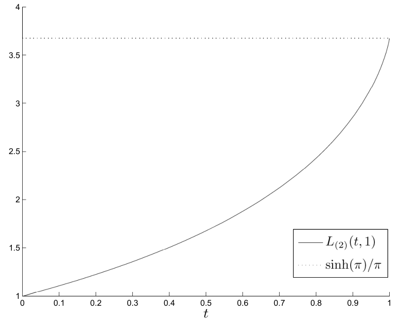
Refer to caption
Figure 2. Plot of ℒ(2)​(t,1)\mathcal{L}_{(2)}(t,1) versus tt

(recall the 1/t1/t factors in (25) are absorbed into Haar integrators). A simulation diagram for this realization suitable for Matlab’s Simulink simulation software is shown Figure 1. Setting θ=1\theta=1 and using Simulink’s default integration routine ode45 (Dormand-Prince method [10]) with a variable step size lower bounded by 10−810^{-8}, Figure 2 was generated showing ℒ(2)​(t,1)=F(x0​x1)∗​[Li0]​(t)\mathcal{L}_{(2)}(t,1)=F_{(x_{0}x_{1})^{\ast}}[\mathrm{Li}_{0}](t) as a function of tt. In particular, it was found numerically that ℒ(2)​(1,1)≈3.6695\mathcal{L}_{(2)}(1,1)\approx 3.6695, which compares favorably to the theoretical value derived from (5):

ℒ(2)​(1,1)=∑n=0∞ζ⁡({2}n)=∑n=0∞π2​n+1(2​n+1)n=sinh⁡(π)π=3.6761.\mathcal{L}_{(2)}(1,1)=\sum_{n=0}^{\infty}\zeta(\{2\}^{n})=\sum_{n=0}^{\infty}\frac{\pi^{2n+1}}{(2n+1)^{n}}=\frac{\sinh(\pi)}{\pi}=3.6761.

Better estimates can be found by more carefully addressing the singularities at the boundary conditions t=0t=0 and t=1t=1 in the Haar integrators.

Example 3.

In order to validate (8), the identity (9) is checked numerically. Since the generating functions ℒ(4)\mathcal{L}_{(4)} and ℒ(3,1)\mathcal{L}_{(3,1)} are periodic, Theorem 4 applies. For 𝐬=(4)\mathbf{s}=(4) the corresponding bilinear realization is

N0=N0​(4)=[0100001000010000],N1=N1​(4)=[000000000000θ4000],z⁡(0)=CT=[1000].N_{0}=N_{0}(4)=\left[\begin{array}[]{cccc}0&1&0&0\\ 0&0&1&0\\ 0&0&0&1\\ 0&0&0&0\end{array}\right],\;\;N_{1}=N_{1}(4)=\left[\begin{array}[]{cccc}0&0&0&0\\ 0&0&0&0\\ 0&0&0&0\\ \theta^{4}&0&0&0\end{array}\right],\;\;z(0)=C^{T}=\left[\begin{array}[]{c}1\\ 0\\ 0\\ 0\end{array}\right].
Refer to caption
Figure 3. Plot of ℒ(4)​(t,θ)−ℒ(3,1)​(t,2​θ)\mathcal{L}_{(4)}(t,\theta)-\mathcal{L}_{(3,1)}(t,\sqrt{2}\theta) versus tt for different values of θ\theta

For 𝐬=(3,1)\mathbf{s}=(3,1) the bilinear realization is

N0=[0100001000000000],N1=[000000000001θ4000],z⁡(0)=CT=[1000].N_{0}=\left[\begin{array}[]{ccc|c}0&1&0&0\\ 0&0&1&0\\ 0&0&0&0\\ \hline\cr 0&0&0&0\end{array}\right],\;\;N_{1}=\left[\begin{array}[]{c|ccc}0&0&0&0\\ 0&0&0&0\\ 0&0&0&1\\ \hline\cr\theta^{4}&0&0&0\end{array}\right],\;\;z(0)=C^{T}=\left[\begin{array}[]{c}1\\ 0\\ 0\\ 0\end{array}\right].

These two dynamical systems were simulated using Haar integrators in Simulink and the difference (9) was computed as a function of tt as shown in Figure 3. As expected, this difference is very close to zero when t=1t=1 no matter how the parameter θ\theta is selected. This is pretty convincing numerical evidence supporting (8), which as discussed in the introduction is known to be true.

Example 4.

Now the method is applied to the generating functions behind the Hoffman conjecture (10). In this case, each multiple polylogarithm has non-periodic components, so Theorem 6 has to be applied three times. The realization for ℒ(2,1,{2},3)​(t,θ)\mathcal{L}_{(2,1,\{2\},3)}(t,\theta) was presented in Example 1. Following a similar approach, the realization for ℒ({2},2,2,2)​(t,θ)\mathcal{L}_{(\{2\},2,2,2)}(t,\theta) and ℒ({2},3,3)​(t,θ)\mathcal{L}_{(\{2\},3,3)}(t,\theta) are, respectively,

N0=[0100000000000000010000000000000001000000000000000],N1=[0000000θ201000000000000000100000000000000010000000],z⁡(0)=[1000001],CT=[1000000]N_{0}=\left[\begin{array}[]{cc|cccc|c}0&1&0&0&0&0&0\\ 0&0&0&0&0&0&0\\ \hline\cr 0&0&0&1&0&0&0\\ 0&0&0&0&0&0&0\\ 0&0&0&0&0&1&0\\ 0&0&0&0&0&0&0\\ \hline\cr 0&0&0&0&0&0&0\end{array}\right],\;N_{1}=\left[\begin{array}[]{cc|cccc|c}0&0&0&0&0&0&0\\ \theta^{2}&0&1&0&0&0&0\\ \hline\cr 0&0&0&0&0&0&0\\ 0&0&0&0&1&0&0\\ 0&0&0&0&0&0&0\\ 0&0&0&0&0&0&1\\ \hline\cr 0&0&0&0&0&0&0\end{array}\right],\;z(0)=\left[\begin{array}[]{c}1\\ 0\\ \hline\cr 0\\ 0\\ 0\\ 0\\ \hline\cr 1\end{array}\right],\;C^{T}=\left[\begin{array}[]{c}1\\ 0\\ \hline\cr 0\\ 0\\ 0\\ 0\\ \hline\cr 0\end{array}\right]

and

N0=[0100000001000000000000000100000001000000000000000],N1=[0000000θ200000000010000000000000000000000010000000],z⁡(0)=[1000001],CT=[1000000].N_{0}=\left[\begin{array}[]{cc|cccc|c}0&1&0&0&0&0&0\\ 0&0&1&0&0&0&0\\ \hline\cr 0&0&0&0&0&0&0\\ 0&0&0&0&1&0&0\\ 0&0&0&0&0&1&0\\ 0&0&0&0&0&0&0\\ \hline\cr 0&0&0&0&0&0&0\end{array}\right],\;N_{1}=\left[\begin{array}[]{cc|cccc|c}0&0&0&0&0&0&0\\ \theta^{2}&0&0&0&0&0&0\\ \hline\cr 0&0&0&1&0&0&0\\ 0&0&0&0&0&0&0\\ 0&0&0&0&0&0&0\\ 0&0&0&0&0&0&1\\ \hline\cr 0&0&0&0&0&0&0\end{array}\right],\;z(0)=\left[\begin{array}[]{c}1\\ 0\\ \hline\cr 0\\ 0\\ 0\\ 0\\ \hline\cr 1\end{array}\right],\;C^{T}=\left[\begin{array}[]{c}1\\ 0\\ \hline\cr 0\\ 0\\ 0\\ 0\\ \hline\cr 0\end{array}\right].
Refer to caption
Figure 4. Plot of ℒ({2},2,2,2)​(t,θ)+2​ℒ({2},3,3)​(t,θ)−ℒ(2,1,{2},3)​(t,θ)\mathcal{L}_{(\{2\},2,2,2)}(t,\theta)+2\mathcal{L}_{(\{2\},3,3)}(t,\theta)-\mathcal{L}_{(2,1,\{2\},3)}(t,\theta) versus tt for different values of θ\theta

.

These dynamical systems were simulated to estimate numerically the left-hand side of (11) as shown in Figure 4. As in the previous example, the case where t=1t=1 is of primary interest. This value is again very close to zero for every choice of θ\theta tested. It is highly likely therefore that the Hoffman conjecture is true.

5. Conclusions

A systematic way was given to numerically evaluate the generating function of periodic multiple polylogarithm using Chen–Fliess series with rational generating series. The method involved mapping the corresponding Chen–Fliess series to a bilinear dynamical system, which could then be simulated numerically using Haar integration. A standard form for such a realization was given, and the method was generalized to the case where the multiple polylogarithm could have non-periodic components. The method was also described in the setting of dendriform algebras. Finally, the technique was used to numerically validate the Hoffman conjecture.

Acknowledgements

The first author is supported by Ramón y Cajal research grant RYC-2010-06995 from the Spanish government. The second author was supported by grant SEV-2011-0087 from the Severo Ochoa Excellence Program at the Instituto de Ciencias Matemáticas in Madrid, Spain. This research was also supported by a grant from the BBVA Foundation.

References

  • [1] T. Aoki, Y. Kombu, and Y. Ohno, A generating function for sums of multiple zeta values and its applications, Proc. AMS, 136 (2008) 387––395.
  • [2] J. Berstel and C. Reutenauer, Noncommutative Rational Series with Applications, Cambridge University Press, Cambridge, UK, 2010.
  • [3] J. M. Borwein, D. M. Bradley, D. J. Broadhurst, and P. Lisonek, Combinatorial aspects of multiple zeta values, Electron. J. Combin., 5 (1998) R38 (12 pp).
  • [4] J. M. Borwein, D. M. Bradley, D. J. Broadhurst, and P. Lisonek, Special values of multidimensional polylogarithms, Trans. Amer. Math. Soc., 353 (2001) 907–941.
  • [5] D. Bowman and D. M. Bradley, Multiple polylogarithms: A brief survey, in Q-series with Applications to Combinatorics, Number Theory, and Physics: A Conference on Q-series with Applications to Combinatorics, Number Theory, and Physics, B. C. Berndt and K. Ono, Eds., AMS, Providence, RI, 2001, pp. 71–92.
  • [6] J. M. Borwein and W. Zudilin, Math honours: Multiple zeta values, available at https://carma.newcastle. edu.au/MZVs/mzv.pdf.
  • [7] R. W. Brockett, On the algebraic structure of bilinear systems, in Theory and Applications of Variable Structure Systems, R. Mohler and R. Ruberti, Eds., Academic Press, New York, 1972, pp. 153–168.
  • [8] P. D’Alessandro, A. Isidori, and A. Ruberti, Realization and structure theory of bilinear dynamical systems, SIAM J. Control, 12 (1974) 517–535.
  • [9] H. T. Dorissen, Canonical forms for bilinear systems, Systems Control Lett., 13 (1989) 153–160.
  • [10] J. R. Dormand and P. J. Prince, A family of embedded Runge-Kutta formulae, J. Comput. Appl. Math., 6 (1980), 19–26.
  • [11] L. A. Duffaut Espinosa, W. S. Gray, and K. Ebrahimi-Fard, Dendriform-Tree Setting for Fully Non-commutative Fliess Operators, Proc. 53rd IEEE Conference on Decision and Control, Los Angeles, CA, 2014, pp. 4814–4819. arXiv:1409.0059v1 [math.CO]
  • [12] L. A. Duffaut Espinosa, W. S. Gray, and K. Ebrahimi-Fard, Dendriform-Tree Setting for Fully Non-commutative Fliess Operators, IMA J. Math. Control Inform., to appear.
  • [13] K. Ebrahimi-Fard and D. Manchon, Dendriform equations, J. Algebra, 322 (2009) 4053–4079.
  • [14] D. L. Elliott, Bilinear Control Systems, Springer, Dordrecht, 2009.
  • [15] M. Fliess, Fonctionnelles causales non linéaires et indéterminées non commutatives, Bull. Soc. Math. France, 109 (1981) 3–40.
  • [16] W. S. Gray and Y. Wang, Fliess operators on LpL_{p} spaces: Convergence and continuity, Systems Control Lett., 46 (2002) 67–74.
  • [17] V. Hoseaux, G. Jacob, N. E. Oussous, and M. Petitot, A Complete Maple package for noncommutative rational power series, in Computer Mathematics: Proceedings of the Sixth Asian Symposium, Beijing, China, Z. Li and W. Y. Sit, Eds., World Scientific, 2003, pp. 174–188.
  • [18] K. Ihara, M. Kaneko, and D. Zagier, Derivation and double shuffle relations for multiple zeta values, Compositio Math., 142 (2006) 307–338.
  • [19] H. J. Sussmann, Minimal realizations and canonical forms for bilinear systems, J. Franklin Inst., 301 (1976) 593–604.
  • [20] I. M. Winter-Arboleda, W. S. Gray, and L. A. Duffaut Espinosa, Fractional Fliess operators: Two approaches, Proc. 49th Conf. Information Sciences and Systems, Baltimore, MD, 2015.
  • [21] M. Zakrzewski and H. Żoładek, Linear differential equations and multiple zeta-values. I. Zeta(2), Fund. Math., 210 (2010) 207–242.
  • [22]  , Linear differential equations and multiple zeta-values. II. A generalization of the WKB method, J. Math. Anal. Appl., 383 (2011) 55–70.
  • [23]  , Linear differential equations and multiple zeta-values. III. Zeta(3), J. Math. Phys., 53 013507 (2012).
  • [24] H. Żoładek, Note on multiple zeta-values, Bul. Acad. Ştiinţe Repub. Mold. Mat., 43 (2003) 78–82.
  • [25] W. Zudilin, Algebraic relations for multiple zeta values, Russian Math. Surveys, 58 (2003) 1–29.