Optimal regularized inverse matrices
for
inverse problems
Abstract
In this paper, we consider optimal low-rank regularized inverse matrix approximations and their applications to inverse problems. We give an explicit solution to a generalized rank-constrained regularized inverse approximation problem, where the key novelties are that we allow for updates to existing approximations and we can incorporate additional probability distribution information. Since computing optimal regularized inverse matrices under rank constraints can be challenging, especially for problems where matrices are large and sparse or are only accessable via function call, we propose an efficient rank-update approach that decomposes the problem into a sequence of smaller rank problems. Using examples from image deblurring, we demonstrate that more accurate solutions to inverse problems can be achieved by using rank-updates to existing regularized inverse approximations. Furthermore, we show the potential benefits of using optimal regularized inverse matrix updates for solving perturbed tomographic reconstruction problems.
Keywords: ill-posed inverse problems, low-rank matrix approximation, regularization, Bayes risk
AMS: 65F22, 15A09, 15A29
1 Introduction
Optimal low-rank inverse approximations play a critical role in many scientific applications such as matrix completion, machine learning, and data analysis [38, 14, 26]. Recent theoretical and computational developments on regularized low-rank inverse matrices have enabled new applications, such as for solving inverse problems [9]. In this paper, we develop theoretical results for a general case for finding optimal regularized inverse matrices (ORIMs), and we propose novel uses of these matrices for solving linear ill-posed inverse problems of the form,
| (1) |
where is the desired solution, models the forward process, is additive noise, and is the observed data. We assume that is very large and sparse, or that cannot be formed explicitly, but matrix vector multiplications with are feasible (e.g., can be an object or function handle). Furthermore, we are interested in ill-posed inverse problems, whereby small errors in the data may result in large errors in the solution [19, 23, 37], and regularization is needed to stabilize the solution.
Next, we provide a brief introduction to regularization and ORIMs, followed by a summary of the main contributions of this work. Various forms of regularization have been proposed in the literature, including variational methods [31, 35] and iterative regularization, where early termination of an iterative methods provides a regularized solution [21, 20]. Optimal regularized inverse matrices have been proposed for solving inverse problems and have been studied in both the Bayes and empirical Bayes framework [8, 6, 9]. Let be an initial approximation matrix (e.g., in previous works). Then treating and as random variables, the goal is to find a matrix that gives a small reconstruction error. That is, should be small for some given error measure . In this paper, we consider to be the squared Euclidean norm, and we seek an optimal matrix that minimizes the expected value of the errors with respect to the joint distribution of and . Hence, the problem of finding an ORIM can be formulated as
| (2) |
This problem is often referred to as a Bayes risk minimization problem [4, 36]. Especially for large scale problems, it may be advisable to include further constraints on such as sparsity, symmetry, block or cyclic structure, or low-rank structure. Here, we will focus on matrices of low-rank. Once computed, ORIM has mainly been used to efficiently solve linear inverse problems in an online phase as data becomes available and requires therefore only a matrix-vector multiplication .
Overview of our contributions
First, we derive a closed-form solution for problem (2) under rank constraints with uniqueness conditions. The two key novelties are that we include matrix , thereby allowing for updates to existing regularized inverse matrices, and we incorporate additional information regarding the distribution of . More specifically, we allow non-zero mean for the distribution of and show that our results reduce to previous results in [9] that assume zero mean and . These extension are not trivial and require a different approach than [9] for the proof. Second, we describe an efficient rank-update approach for computing a global minimizer of (2) under rank constraints, that is related to but different than the approach described in [7] where training data was used as a substitute for knowledge of the forward model. We demonstrate the efficiency and accuracy of the rank-update approach, compared to standard SVD-based methods, for solving a sequence of ill-posed problems.
Third, we propose novel uses of ORIM updates in the context of solving inverse problems. An example from image deblurring demonstrates that updates to existing regularized inverse matrix approximations such as the Tikhonov reconstruction matrix can lead to more accurate solutions. Also, we use an example from tomographic image reconstruction to show that ORIM updates can be used to efficiently and accurately solve perturbed inverse problems. This contribution has significant implications for further research development, ranging from use within nonlinear optimization schemes to preconditioner updates.
The key benefits of using ORIMs for solution updates and for solving inverse problems are that (1) we approximate the regularized inverse directly, so reconstruction or application requires only a matrix-vector multiplication rather than a linear solve; (2) our matrix inherently incorporates regularization; (3) ORIMs and ORIM updates can be computed for any general rectangular matrix , even if is only available via a function call, making it ideal for large-scale problems.
The paper is organized as follows. In Section 2, we provide preliminaries to establish notation and summarize important results from the literature. Then, in Section 3, we derive a closed form solution to problem (2) under rank constraints and provide uniqueness conditions (see Theorem 3.3 for the main result). For large-scale problems, computing an ORIM according to Theorem 3.3 may be computationally prohibitive, so in Section 4, we describe a rank-update approach for efficient computation. Finally, in Section 5 we provide numerical examples from image processing that demonstrate the benefits of ORIM updates. Conclusions and discussions are provided in Section 6.
2 Background
In this section, we begin with preliminaries to establish notation.
Given a matrix with rank , let denote the singular value decomposition (SVD) of , where and are orthogonal matrices that contain the left and right singular vectors of , respectively. Diagonal matrix contains the singular values and zeros on its main diagonal. The truncated SVD approximation of rank of is denoted by where and contain the first vectors of and respectively, and is the principal submatrix of . The TSVD approximation is unique if and only if . Furthermore, the Moore-Penrose pseudoinverse of is given by .
Next we show that the problem of finding an optimal regularized inverse matrix (ORIM) (i.e., a solution to (2)) is equivalent to solving a matrix approximation problem. That is, assuming and are random variables, the goal is to find a matrix such that we minimize the expected value of the squared 2-norm error, i.e., , where
is often referred to as the Bayes risk.
Lets further assume that and are independent random variables with , the covariance matrix is symmetric positive definite, , and . First, due to the independence of and and since , we can rewrite the Bayes risk as
Then using the property of the quadratic form [33], , where denotes the trace, is symmetric, and ,
with being any symmetric factorization, e.g., Cholesky factorization. Using the cyclic property of the trace leads to
where denotes the Frobenius norm. Next we rewrite in terms of only one Frobenius norm. Let , then using the identities of the Frobenius and the vector 2-norm, as well as applying Kronecker product properties, we get
| (3) |
Thus, minimizing the Bayes risk in problem (2) is equivalent to minimizing (3). Notice that so far we have not imposed any constraints on . Although various constraints can be imposed on , here we consider to be of low-rank, i.e., for some . Hence the low-rank matrix approximation problem of interest in this paper is
| (4) |
We will provide a closed form solution for (4) in Section 3, but it is important to remark that special cases of this problem have been previously studied in the literature. For example, a solution for the case where and was provided in [9] that uses the generalized SVD of . If, in addition, we assume then an optimal regularized inverse matrix of at most rank reduces to a truncated-Tikhonov matrix [9],
| (5) |
where . Moreover, this is the unique global minimizer for
| (6) |
if and only if .
3 Low-rank optimization problem
The goal of this section is to derive the unique global minimizer for problem (4), under suitable conditions. We actually consider a more general problem, as stated in Theorem 3.3, where with Our proof uses a special case of Theorem 2.1 from Friedland & Torokhti [16] that is provided here for completeness.
Theorem 3.1.
Let matrices and with be given. Then
is a solution to the minimization problem
having a minimal . This solution is unique if and only if either
or
Proof.
See [16]. ∎
To get to our main result we first provide the following Lemma.
Lemma 3.2.
Let with and parameter , nonzero if . Let further with for and for . Then the SVD of is given by , where
with arbitrary and satisfying and
Proof.
Let the SVD of be given. First, notice that the singular values , where defines the -th eigenvalue of the matrix with . Since the eigenvalue decomposition of is given by
| (7) |
we have
with , where
and
Notice that, is invertible if or . By equation (7) the left singular vectors of correspond to the left singular vectors of , i.e., . As for the right singular vectors let
with , and . Then
and and . The matrices and are any matrices satisfying and or equivalently . ∎
Next, we provide a main result of our paper.
Theorem 3.3.
Given matrices , , and , with , , let index and parameter , nonzero if . Define . If , then a global minimizer of the problem
| (8) |
is given by
| (9) |
where symmetric matrix has eigenvalue decomposition with eigenvalues ordered so that for , and contains the first columns of . Moreover, is the unique global minimizer of (8) if and only if .
Proof.
We will use Theorem 3.1 where and . Let
with
denote the generalized SVD of and let be defined by with its SVD given by . Then , where and . Using Lemma 3.2, the SVD of is given by
with
and appropriately defined and . Notice that is invertible and , if either or . Also acknowledge that . Thus, the pseudoinverse of is given by
and
Let , then
| (10) |
Notice that , since by assumption. Then, let symmetric matrix have eigenvalue decomposition with eigenvalues ordered so that for . Next we proceed to get an SVD of ,
with
where and remaining matrices are defined accordingly. Then equating the SVD of with (10) and using a similar argument as in Lemma 3.2, we get
and
Since (the principal submatrix of ) is invertible, the transpose of the first columns of have the form,
and the best rank approximation of is given by
Finally, using Theorem 3.1 we find that all global minimizers of with rank at most can be written as
where is a unique global minimizer of (8) if and only if since this condition makes the choice of unique. ∎
4 Efficient methods to compute ORIM
The computational cost to compute a global minimizer according to Theorem 3.3 requires the computation of a GSVD of , an SVD of , and a partial eigenvalue decomposition of . For large-scale problems this may be computational prohibitive, so we seek an alternative approach to efficiently compute ORIM . In the following we decompose the optimization problem into smaller subproblems and use efficient methods to solve the subproblems. The optimality of our update approach is verified by the following corollary of Theorem 3.3.
Corollary.
The significance of the corollary is as follows. Assume we are given a rank approximation and we are interested in updating our approximation to a rank approximation . To calculate the optimal rank approximation , we just need to solve a rank optimization problem of the form (11) and then update the solution, . Thus, computing a rank ORIM matrix can be achieved by solving a sequence of smaller rank problems and updating the solutions. Algorithm 1 describes such an rank-1 update approach.
The main question in Algorithm 1 is how to efficiently solve the optimization problem in line 3. First, we reformulate the rank-1 constraint by letting where and and defining and . Then , and the optimization problem in line 3 of Algorithm 1 reads
|
|
(12) |
Although standard optimization methods could be used, care must be taken since this quartic problem is of dimension and ill-posed since the decomposition is not unique. Notice that for fixed , optimization problem (12) is quadratic and convex in and vise versa. Thus, we propose to use an alternating direction optimization approach. Assume , , and , then the partial optimization problems resulting from (12) are ensured to have unique minimizers
| (13) |
and
Notice that computing in (13) only requires matrix-vector products, while computing requires a linear solve. Since decomposition is not unique, we propose to select the computationally convenient decomposition where and . This results in a simplified formula for , i.e.,
| (14) |
Noticing that (14) is just the normal equations solution to the following least squares problem,
| (15) |
we propose to use a computationally efficient least squares solver such as LSQR [29, 30], where various methods can be used to exploit the fact that the coefficient matrix remains constant [5, 3]. In addition, quasi Newton methods may improve efficiency by taking advantage of a good initial guess and a good approximation on the inverse Hessian [28], but such comparisons are beyond the scope of this paper.
The alternating direction approach to compute a rank-1 update is provided in Algorithm 2.
In summary, our proposed method to compute low-rank ORIM combines Algorithms 1 and 2. An efficient Matlab implementation can be found at the following website:
\urlhttps://github.com/juliannechung/ORIM.git
Before providing illustrations and examples of our method, we make a few remarks regarding numerical implementation.
- 1.
Storage. Algorithmically need never be constructed, as we only require matrices and . This decomposition is storage preserving as long as and is ideal for problems where is too large to compute or can only be accessed via function call.
- 2.
Stopping criteria. For Algorithm 1, the specific rank for may be user-defined, but oftentimes such information is not available a priori. However, the rank-1 update approach allows us to track the improvement in the function value from rank to rank . Then an approximation of rank is deemed sufficient when , where our default tolerance is . Standard stopping criteria [17] can be used for Algorithm 2. In particular, we track improvement in the function values , track changes in the arguments and , and set a maximum iteration. Our default tolerance is .
- 3.
Efficient function evaluations. Rather than computing the function value from scratch at each iteration (e.g., for determining stopping criteria), efficient updates can be done by observing that
where . Since function evaluations are only relevant for the stopping criteria, they can be discarded, if desired, or approximated using trace estimators [1].
- 4.
Initialization. Equation (13) requires an initial guess for . One uninformed choice may be , and another option is to select orthogonal to , i.e., with chosen at random.
- 5.
Symmetry. If and are symmetric, our rank-1 update approach could be used to compute a symmetric ORIM , but the alternating direction approach should be replaced by an appropriate method for minimizing a quartic in .
- 6.
Covariance matrix. Since in our rank update approach only occurs in the product and since , our algorithm can work directly with the covariance matrix. Thus, a symmetric factorization does not need to be computed, which is important for various classes of covariance kernels [32].
5 Numerical Results
In this section, we provide three experiments that not only highlight the benefits of ORIM updates but also demonstrate new approaches for solving inverse problems that use ORIM updates. In Experiment 1, we use an inverse heat equation to investigate the efficiency and accuracy of our update approach. Then in Experiment 2, we use an image deblurring example to show that more accurate solutions to inverse problems can be achieved by using ORIM rank-updates to existing regularized inverse matrices. Lastly, in Experiment 3, we show that ORIM updates can be used in scenarios where perturbed inverse problems need to be solved efficiently and accurately.
5.1 Experiment 1: Efficiency of ORIM rank update approach
The goal of this example is to highlight our new result in Theorem 3.3 and to verify the accuracy and efficiency of the update approach described in Section 4. We consider a discretized (ill-posed) inverse heat equation derived from a Volterra integral equation of the first kind on with kernel , where . Coefficient matrix is and is significantly ill-posed for . We generate using the Regularization Tools package [22].
As a first study, we compare ORIM with other commonly used regularized inverse matrices. Notice that is fully determined by , and .
For this illustration, we select and to be realizations of random matrices whose entries are i.i.d. standard normal , and we select and . Then we compute ORIM as in Equation (9) for various ranks and plot the function values in Figure 1. For comparison, we also provide function values for other commonly used rank- reconstruction matrices, including the TSVD matrix, the truncated Tikhonov matrix (5) (TTik), and the matrix provided from Theorem 1 of [9], here referred to as ORIM0. Notice that TTik and ORIM0 matrices are just special cases of ORIM where and for TTik and and for ORIM0. Figure 1 shows that, as expected, the function values for ORIM are smallest for all computed ranks.
We also verified our proposed rank-update approach by comparing function values computed with the rank update approach to those from Theorem 3.3. We observed that the relative absolute errors remained below for all computed ranks , making the plot of the function values for the update approach indistinguishable from the solid line in Figure 1. Thus, we omit it for clarity of presentation.
Next, we illustrate the efficiency of our rank update approach for solving a sequence of ill-posed inverse problems. Such scenarios commonly occur in nonlinear optimization problems such as variable projection methods where nonlinear parameters are moderately changing during the optimization process [28, 18]. Consider again the inverse heat equation, and assume that we are given a sequence of matrices , where the matrices depend nonlinearly on parameter , and we are interested in solving a sequence of problems, for various .
For each problem in the sequence, one could compute a Tikhonov solution , where
but this approach requires an SVD of for each . We consider an alternate approach, where the SVD is computed once for a fixed and then ORIM updates are used to obtain improved regularized inverse matrices for other ’s. This approach relies on the fact that small perturbations in lead to small rank updates in its inverse [34].
Again for the inverse heat equation we use and and choose and . We select equidistant values for , , and let be the Tikhonov reconstruction matrix corresponding to . Then for all other problems in the sequence, we compute reconstructions as
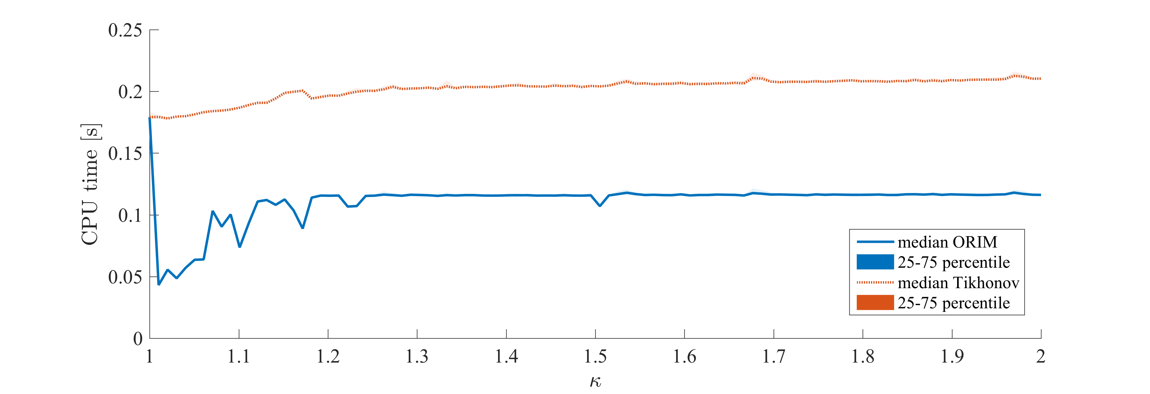
where , where and are the low rank ORIM updates corresponding to . We use a tolerance . In Figure 2, we report computational timings for the ORIM rank update approach, compared to the SVD, and in Figure 3 we provide corresponding relative reconstruction errors, computed as , where is and approximation of (here, and ). We observe that the ORIM update approach requires approximately half the required CPU time compared to the SVD, and the ORIM update approach can produce relative reconstruction errors that are comparable to and even slightly better than Tikhonov. However, we also note potential disadvantages of our approach. In particular, the SVD can be more efficient for small , although ORIM updates are significantly faster for larger problems (results not shown). Also, using different noise levels in each problem or taking larger changes in may result in higher CPU times and/or higher reconstruction errors for the update approach. We assume that the noise levels and problems are not changing significantly.

5.2 Experiment 2: ORIM Updates to Tikhonov
Here we consider a classic image deblurring problem, where the model is given in (1) where represents the desired image, models the blurring process, and is the blurred, observed image. The true image was taken to be the -th slice of the 3D MRI image dataset that is provided in MATLAB, which is pixels. We assume spatially invariant blur, where the point spread function (PSF) is a box-car blur. We assume reflexive boundary conditions for the image. Since the PSF is doubly symmetric, blur matrix is highly structured and its singular value decomposition is given by , where here and represent the 2D discrete cosine transform (DCT) matrix and inverse 2D DCT matrix respectively [24]. Here we use the RestoreTools package [27]. Noise was generated from a normal distribution, with zero mean, and scaled such that the noise level was . The true and observed images, along with the PSF, are provided in Figure 4.
 |
 |
 |
| (a) True image | (b) Observed, blurred image | (c) Point spread function |
As an initial regularized inverse approximation, we use a Tikhonov reconstruction matrix, , where regularization parameter was selected to provide minimal reconstruction error. That is, we used , which corresponded to the minimum of error function, . Although this approach uses the true image (which is not known in practice), our goal here is to demonstrate the improvement that can be obtained using the rank-update approach. In practice, a standard regularization parameter selection method such as the generalized cross-validation could be used, which for this problem gave . The Tikhonov reconstruction, , is provided in Figure 5(a) along with the computed relative reconstruction error.
Next we consider various ORIM updates to and evaluate corresponding reconstructions. For the mean vector , we use the image shown in Figure 5(b), which was obtained by averaging images slices 8–22 of the MRI stack (omitting slice 15, the image of interest). For efficient computations and simplicity, we assume is diagonal with variances proportional to , we choose, ; the matrix is defined accordingly. We compute ORIM updates to according to Algorithm 1 for the following cases of :
| (16) |
We refer to these matrix updates as , , and respectively, where is a rank-1 matrix and and are matrices of rank . Image reconstructions were obtained via matrix-vector multiplication,
and are provided in Figure 5(c)–(e). Corresponding relative reconstruction errors are also provided.
 |
 |
| (a) Tikhonov, , | (b) Mean image, |
 |
 |
 |
| (c) , | (d) , | (e) , |
Furthermore, absolute error images (in inverted colormap so that black corresponds to larger reconstruction error) in Figure 6 show that the errors for the ORIM updated solution have smaller and more localized errors than the initial Tikhonov reconstruction.
 |
 |
| (a) Tikhonov | (b) |
We repeated this experiment times, each time with a different noise realization in and provide the distribution of the corresponding relative reconstruction errors in Figure 7. Additionally, for each of these approaches, we provide the average reconstruction error, along with the standard deviation over all noise realizations in Table 1. It is evident from these experiments that ORIM rank-updates to the Tikhonov reconstruction matrix can lead to reconstructions with smaller relative errors and allows users to easily incorporate prior knowledge regarding the distributions of and .

| mean standard deviation | |
|---|---|
| Tikhonov | |
| ORIM update, | |
| ORIM update, | |
| ORIM update, |
We then applied our reconstruction matrices, to the other images in the MRI stack and provide the relative reconstruction errors in Figure 8. We observe that in general, all of the reconstruction matrices provide fairly good reconstructions, with smaller relative errors corresponding to images that are most similar to the mean image. Some of the true images were indeed included in the mean image. Regardless, our goal here is to illustrate that ORIM update matrices can be effective and efficient, if a good mean image and/or covariance matrix are provided. Other covariance matrices can be easily incorporated in this framework, but comparisons are beyond the scope of this work.
5.3 Experiment 3: ORIM updates for perturbed problems
Last, we consider an example where ORIM updates to existing regularized inverse matrices can be used to efficiently solve perturbed problems. That is, consider a linear inverse problem such as (1) where a good regularized inverse matrix denoted by can be obtained. Now, suppose is modified slightly (e.g., due to equipment setup or a change in model parameters), and a perturbed linear inverse problem
| (17) |
must be solved. We will show that as long as the perturbation is not too large, a good solution to the perturbed problem can be obtained using low-rank ORIM updates to . This is similar to the scenario described in Experiment 1, but here we use an example from 2D tomographic imaging, where the goal is to estimate an image or object , given measured projection data. The Radon transform can be used to model the forward process, where the Radon transform of is given by
| (18) |
where is the Dirac delta function. Figure 9 illustrates the basic tomographic process.

The goal of the inverse problem is to compute a (discretized) reconstruction of the image , given projection data that is collected at various angles around the object. The projection data, when stored as an image, gives the sinogram. In Figure 10 (a), we provide the true image which is a image of the Shepp-Logan phantom, and two sinograms are provided in Figure 10 (b) and (c), where the rows of the image contain projection data at various angles. In particular, for this example, we take projection images at degree intervals from to degrees (i.e., the sinogram contains rows). In order to deal with boundary artifacts, we pad the original image with zeros.
 |
 |
 |
| (a) True image | (b) Sinogram 1 | (c) Sinogram 2 |
The discrete tomographic reconstruction problem can be modeled as (1) where represents the (vectorized) desired image, models the tomographic process, and is the (vectorized) observed sinogram. For this example, we construct
where is a sparse matrix that represents rotation of the image for the -th angle, whose entries were computed using bilinear interpolation as described in [10, 11], and is a Kronecker product that approximates the integration operation. It is worth mentioning that in typical tomography problems, is never created, but rather accessed via projection and backprojection operations [15]. Our methods also work for scenarios where represents a function call or object, but our current approach allows us to to build the sparse matrix directly. White noise is added to the problem at relative noise level .
Since has no obvious structure to exploit, we use iterative reconstruction methods to get an initial reconstruction matrix. This mimics a growing trend in tomography where reconstruction methods have shifted from filtered back projection approaches to iterative reconstruction methods [25, 2]. Furthermore, these iterative approaches are ideal for problems such as limited angle tomogography or tomosynthesis, where the goal is to obtain high quality images while reducing the amount of radiation to the patient [13, 12]. In this paper, we define a regularized inverse matrix in terms of a partial Golub-Kahan bidiagonalization. That is, given a matrix and vector the Golub-Kahan process iteratively transforms matrix to upper-bidiagonal form , with initializations , and . After steps of the Golub-Kahan bidiagonalization process, we have matrices , , and bidiagonal matrix
such that
| (19) |
It is worth noting that in exact arithmetic, the -th LSQR [29, 30] iterate is given by . Thus, we define to be a regularized inverse matrix for the original problem, where corresponds to minimal reconstruction error for the original problem. See Figure 11 for the relative error plot for the original problem.
The goal of this illustration is to show that a low-rank ORIM update to can be used to solve a perturbed problem. Thus, we created a perturbed problem (17), where and were created with slightly shifted projection angles. Again, we take projection images at degree intervals, but this time the angles ranged from to degrees. The corresponding sinogram is given in Figure 10(c). A first approach would be to use to reconstruct the perturbed data: . This reconstruction is provided in the top left corner of Figure 12, and it is evident that this is not a very good reconstruction. After a rank-4 update to , where , and , we get a significantly better reconstruction (middle column of Figure 12). For comparison purposes, we provide in the last column the best LSQR reconstruction for the perturbed problem (i.e., corresponding to minimal reconstruction error). Relative reconstruction errors are provided, and corresponding absolute error images are presented on the same scale and with inverted colormap.
Initial, ORIM, LSQR,


6 Conclusions
In this paper, we provide an explicit solution for a generalized rank-constrained matrix inverse approximation problem. We define the solution to be an optimal regularized inverse matrix (ORIM), where we include regularization terms, rank constraints, and a more general weighting matrix. Two main distinctions from previous results are that we can include updates to an existing matrix inverse approximation, and in the Bayes risk minimization framework, we can incorporate additional information regarding the probability distribution of For large scale problems, obtaining an ORIM according to Theorem 3.3 can be computationally prohibitive, so we described an efficient rank-update approach that decomposes the optimization problem into smaller rank subproblems and uses gradient-based methods that can exploit linearity. Using examples from image processing, we showed that ORIM updates can be used to compute more accurate solutions to inverse problems and can be used to efficiently solve perturbed systems, which opens the door to new applications and investigations. In particular, our current research is on incorporating ORIM updates within nonlinear optimization schemes such as variable projection methods, as well as on investigating its use for updating preconditioners for slightly changing systems.
References
- [1] H. Avron and S. Toledo, Randomized algorithms for estimating the trace of an implicit symmetric positive semi-definite matrix, Journal of the ACM (JACM), 58 (2011), pp. 8:1–8:17.
- [2] M. Beister, D. Kolditz, and W. A. Kalender, Iterative reconstruction methods in x-ray ct, Physica medica, 28 (2012), pp. 94–108.
- [3] M. Benzi, Preconditioning techniques for large linear systems: a survey, Journal of Computational Physics, 182 (2002), pp. 418–477.
- [4] B. Carlin and T. Louis, Bayes and Empirical Bayes Methods for Data Analysis, Chapman and Hall/CRC, Boca Raton, 2 ed., 2000.
- [5] K. Chen, Matrix Preconditioning Techniques and Applications, vol. 19, Cambridge University Press, Cambridge, 2005.
- [6] J. Chung and M. Chung, Computing optimal low-rank matrix approximations for image processing, in IEEE Proceedings of the Asilomar Conference on Signals, Systems, and Computers. November 3-6, 2013, Pacific Grove, CA, USA, 2013.
- [7] J. Chung and M. Chung, An efficient approach for computing optimal low-rank regularized inverse matrices, Inverse Problems, 30 (2014), pp. 1–19.
- [8] J. Chung, M. Chung, and D. O’Leary, Designing optimal filters for ill-posed inverse problems, SIAM Journal on Scientific Computing, 33 (2011), pp. 3132–3152.
- [9] J. Chung, M. Chung, and D. P. O’Leary, Optimal regularized low rank inverse approximation, Linear Algebra and its Applications, 468 (2015), pp. 260–269.
- [10] J. Chung, E. Haber, and J. G. Nagy, Numerical methods for coupled super-resolution, Inverse Problems, 22 (2006), pp. 1261–1272.
- [11] J. Chung and J. Nagy, An efficient iterative approach for large-scale separable nonlinear inverse problems, SIAM Journal on Scientific Computing, 31 (2010), pp. 4654–4674.
- [12] J. Chung, J. Nagy, and I. Sechopoulos, Numerical algorithms for polyenergetic digital breast tomosynthesis reconstruction, SIAM Journal on Imaging Sciences, 3 (2010), pp. 133–152.
- [13] J. T. Dobbins III and D. J. Godfrey, Digital x-ray tomosynthesis: current state of the art and clinical potential, Physics in medicine and biology, 48 (2003), p. R65.
- [14] P. Drineas, R. Kannan, and M. Mahoney, Fast Monte Carlo algorithms for matrices II: Computing a low-rank approximation to a matrix, SIAM Journal on Computing, 36 (2007), pp. 158–183.
- [15] T. G. Feeman, Mathematics of Medical Imaging, Springer, 2015.
- [16] S. Friedland and A. Torokhti, Generalized rank-constrained matrix approximations, SIAM Journal on Matrix Analysis and Applications, 29 (2007), pp. 656–659.
- [17] P. Gill, W. Murray, and M. Wright, Practical Optimization, Emerald Group Publishing, Bingley, UK, 1981.
- [18] G. Golub and V. Pereyra, The differentiation of pseudo-inverses and nonlinear least squares whose variables separate, SIAM J. Numer. Anal., 10 (1973), pp. 413–432.
- [19] J. Hadamard, Lectures on Cauchy’s Problem in Linear Differential Equations, Yale University Press, New Haven, 1923.
- [20] M. Hanke, Conjugate Gradient Type Methods for Ill-Posed Problems, Pitman Research Notes in Mathematics, Longman Scientific & Technical, Harlow, Essex, 1995.
- [21] M. Hanke and P. Hansen, Regularization methods for large-scale problems, Surveys on Mathematics for Industry, 3 (1993), pp. 253–315.
- [22] P. Hansen, Regularization tools: A MATLAB package for analysis and solution of discrete ill-posed problems, Numerical Algorithms, 6 (1994), pp. 1–35.
- [23] P. Hansen, Discrete Inverse Problems: Insight and Algorithms, SIAM, Philadelphia, 2010.
- [24] P. Hansen, J. Nagy, and D. O’Leary, Deblurring Images: Matrices, Spectra and Filtering, SIAM, Philadelphia, 2006.
- [25] J. Hsieh, Computed tomography: principles, design, artifacts, and recent advances, SPIE Bellingham, WA, 2009.
- [26] I. Markovsky, Low Rank Approximation: Algorithms, Implementation, Applications, Springer, New York, 2012.
- [27] J. Nagy, K. Palmer, and L. Perrone, Iterative methods for image deblurring: A Matlab object oriented approach, Numerical Algorithms, 36 (2004), pp. 73–93.
- [28] J. Nocedal and S. Wright, Numerical Optimization, Springer, New York, 1999.
- [29] C. Paige and M. Saunders, LSQR: An algorithm for sparse linear equations and sparse least squares, ACM Transactions on Mathematical Software, 8 (1982), pp. 43–71.
- [30] C. C. Paige and M. A. Saunders, Algorithm 583, LSQR: Sparse linear equations and least-squares problems, ACM Trans. Math. Soft., 8 (1982), pp. 195–209.
- [31] L. Rudin, S. Osher, and E. Fatemi, Nonlinear total variation based noise removal algorithms, Physica D, 60 (1992), pp. 259–268.
- [32] A. K. Saibaba, S. Ambikasaran, J. Yue Li, P. K. Kitanidis, and E. F. Darve, Application of hierarchical matrices to linear inverse problems in geostatistics, Oil and Gas Science and Technology-Revue de l’IFP-Institut Francais du Petrole, 67 (2012), p. 857.
- [33] G. A. F. Seber and A. J. Lee, Linear Regression Analysis, vol. 936, John Wiley & Sons, San Francisco, 2012.
- [34] G. W. Stewart, Matrix Algorithms: Volume 2. Eigensystems, vol. 2, SIAM, Philadelphia, 2001.
- [35] A. Tikhonov and V. Arsenin, Solutions of Ill-posed Problems, Winston, 1977.
- [36] V. Vapnik, Statistical Learning Theory, Wiley, San Francisco, 1998.
- [37] C. R. Vogel, Computational Methods for Inverse Problems (Frontiers in Applied Mathematics), SIAM, Philadelphia, 1987.
- [38] J. Ye, Generalized low rank approximations of matrices, Machine Learning, 61 (2005), pp. 167–191.