Four-dimensional black holes with scalar hair in nonlinear electrodynamics
Abstract
We consider a gravitating system consisting of a scalar field minimally coupled to gravity with a self-interacting potential and a U(1) nonlinear electromagnetic field. Solving analytically and numerically the coupled system for both power-law and Born-Infeld type electrodynamics, we find charged hairy black hole solutions. Then, we study the thermodynamics of these solutions and we find that at a low temperature the topological charged black hole with scalar hair is thermodynamically preferred, whereas the topological charged black hole without scalar hair is thermodynamically preferred at a high temperature for power-law electrodynamics. Interestingly enough, these phase transitions occur at a fixed critical temperature and do not depend on the exponent of the nonlinearity electrodynamics.
I Introduction
Hairy black holes are interesting solutions to Einstein’s Theory of Gravity and also to certain types of Modified Gravity Theories. The first attempts to couple a scalar field to gravity was done in an asymptotically flat spacetime finding hairy black hole solutions [1], but it was realized that these solutions were not physically acceptable as the scalar field was divergent on the horizon and stability analysis showed that they were unstable [2]. Also, asymptotically flat black holes with scalar field minimally coupled to gravity were found in [3, 4], which evade the no hair theorems by allowing partially negative self-interacting potential, which is in conflict with the dominant energy condition. Some of these solutions were found to be stable for some parameter range [4]. On the other hand, by introducing a cosmological constant, hairy black hole solutions with a minimally coupled scalar field and a self-interaction potential in asymptotically dS space were found, but unstable [5, 6]. Also, a hairy black hole configuration was reported for scalar field non-minimally coupled to gravity [7], but a perturbation analysis showed the instability of the solution [8, 9]. In the case of a negative cosmological constant, stable solutions were found numerically for spherical geometries [10, 11] and an exact solution in asymptotically AdS space with hyperbolic geometry was presented in [12]. A study of general properties of black holes with scalar hair with spherical symmetry can be found in Ref. [13]. Further hairy solutions were reported in [14, 15, 16, 17, 18, 19, 20, 21, 22] with various properties. Furthermore, charged hairy solutions were also found, for instance in [23], a topological black hole dressed with a conformally coupled scalar field and electric charge was studied. An electrically charged black hole solution with a scalar field minimally coupled to gravity and electromagnetism was presented in [24]. Recently, for a gravitating system consisting of a scalar field minimally coupled to gravity with a self-interacting potential and U(1) electromagnetic field, exact charged hairy black hole solutions with the scalar field which is regular outside the event horizon have been found in [25, 26, 27]. Also, new hairy black hole solutions, boson stars and numerical rotating hairy black hole solutions were discussed [28, 29, 30, 31, 32, 33], as well as time-dependent hairy black holes [34, 35]. For a review of hairy black holes we refer the reader to [36].
In this work, we extend our previous work [18, 25] and we consider a gravitating system consisting of a scalar field minimally coupled to gravity with a self-interacting potential and U(1) nonlinear electromagnetic field. Then, we obtain black hole solutions for power-law and Born-Infeld type electrodynamics and we study the thermodynamics and the phase transitions between hairy charged black holes dressed with a scalar field and no hairy charged black holes, focusing on the effects of the nonlinearity of the Maxwell source. The interest in nonlinear electrodynamics arises with the order to eliminate the problem of infinite energy of the electron by Born and Infeld [37]. Also, nonlinear electrodynamics emerge in the modern context of the low-energy limit of heterotic string theory [38, 39, 40], and play an important role in the construction of regular black hole solutions [41, 42, 43, 44, 45, 46]. Some black holes/branes solutions in a nonlinear electromagnetic field have been investigated for instance in [47, 48, 49, 50, 51, 52, 53, 54] and references therein. The thermodynamics of Einstein-Born-Infeld black holes with a negative cosmological constant was studied in [55] and for a power-law electrodynamic in [56], where the authors showed that a set of small black holes are locally stable by computing the heat capacity and the electrical permittivity. The thermodynamics of Gauss-Bonnet black holes for a power-law electrodynamic was studied in [57]. On the other hand, higher dimensional black hole solutions to Einstein-dilaton theory coupled to Maxwell field were found in [58, 59] and black hole solutions to Einstein-dilaton theory coupled to Born-Infeld and power-law electrodynamics were found in [60, 61].
The phase transitions have been of great interest since the discovery of a phase transition by Hawking and Page in a four-dimensional Schwarzschild AdS background [62]. Witten [63] has extended this four-dimensional transition to arbitrary dimension and provided a natural explanation of a confinement/deconfinement transition on the boundary field theory via the AdS/CFT correspondence. However, phase transitions have recently garnered a great deal of attention motivated mainly by the relationship between the phase transitions and holographic superconductivity [64, 65] in the context of the AdS/CFT correspondence. Furthermore, the effects of nonlinear electrodynamics on the properties of the holographic superconductors have recently been investigated [66, 67, 68, 69, 70, 71, 72, 73, 74, 75]. It is known that these phase transitions can be obtained by considering black holes as states in a same grand canonical ensemble and by comparing the free energy associated with each of them. So, it is necessary to find the conserved charge of the theory. It is worth mentioning that the phase transition phenomena have been analyzed and classified by exploiting Ehrenfest’s scheme [76, 77, 78, 79]. Another point of view to study phase transitions is to consider Bragg-Williams’ construction of a free energy function [80]. Also, it was shown that if the space is flat, then the Reissner-Nordström black hole is thermodynamically preferred, whereas if the space is AdS the hairy charged black hole is thermodynamically preferred at a low temperature [25].
II Four-dimensional black holes with scalar hair in nonlinear electrodynamics
The four-dimensional Einstein-Hilbert action with a scalar field minimally coupled to curvature having a self-interacting potential in the presence of a nonlinear electromagnetic field is
| (1) |
where , with the Newton constant and an arbitrary function of the electromagnetic invariant . The resulting field equations from the above action are
| (2) |
where the energy-momentum tensors and for the scalar and electromagnetic fields are
| (3) |
respectively. Using Eqs. (2) and (3) we obtain the equivalent equation
| (4) |
Now, if we consider the following metric ansatz
| (5) |
where is the metric of the spatial 2 section, which can have a positive, negative or zero curvature, and is the scalar potential of the electromagnetic field. We find the following three independent differential equations
| (6) |
| (7) |
| (8) |
where parameterizes the curvature of the spatial 2-section. So, if we eliminate the potential from the above equations we obtain
| (9) |
| (10) |
In the following, we will work in units where . By considering the scalar field studied in [25],
| (11) |
where is a parameter controlling the behavior of the scalar field and it has the dimension of length, from Eqs. (9) and (11) we determine the function , which reads
| (12) |
Also, from the Maxwell equations
| (13) |
we obtain the following relation
| (14) |
where is an integration constant. We can also determine the metric function replacing (12) and (14) in (10)
| (15) | ||||
To find hairy black hole solutions the differential equations have to be supplemented with the Klein-Gordon equation of the scalar field, which in general coordinates reads
whose solution for the self-interacting potential is
| (16) |
In the following sections we will consider two specific electromagnetic Lagrangians : Power-law and Born-Infeld type electrodynamics.
II.1 Power-law electrodynamics
In this section we consider power-law electrodynamics characterized by the following Lagrangians [81]
| (17) |
where is a rational number and the absolute value ensures that any configuration of electric and magnetic fields can be described by these Lagrangians. One could also consider the Lagrangian without the absolute value and the exponent restricted to being an integer or a rational number with an odd denominator [82]. The sign of the coupling constant will be chosen such that the energy density of the electromagnetic field is positive; that is, the minus component of the electromagnetic energy-momentum tensor must be positive
| (18) |
This condition is guaranteed in the following cases: and or and . In what follows we focus our attention on purely electric field configurations.
From Maxwell equations (14) we obtain
| (19) |
where is an integration constant related to by . So
| (20) |
The integration constant will be chosen in such a way the electric potential goes to zero asymptotically for , and is given by
| (21) |
Thus, for the electric potential behaves as:
| (22) |
where denotes terms that goes to zero at large distances. Eq. (22) shows that the field tends to zero at infinity for and diverges at infinity for and . However, the above solution is not valid for with being an integer. Fortunately, in that case we obtain analytical solutions that we present in the Appendix. We can also determine the metric function replacing (20) in (15). We find
| (23) | ||||
where
| (24) |
and the following redefinition of the integration constant have been taken into account:
| (25) |
and the scalar field potential can be written as
| (26) | ||||
where we have defined
| (27) | ||||
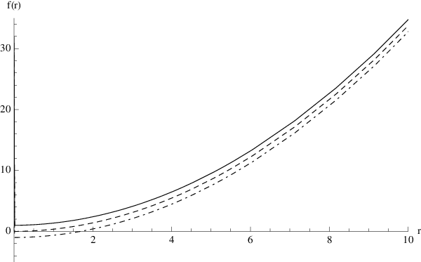
The integral above apparently depends on ; however, it can be shown numerically that the integral does not depend on ; so, in the last line of the above expression we have set for simplicity. Therefore, the potential does not depend on the parameter . We have used the reverse type procedure to obtain the potential, chosen in a way that the solution found from the remaining equations of motion with a metric ansatz and an electric field also solves the Klein-Gordon equation. Then, we can investigate whether our system has a charged hairy black hole solution. In Fig. 1 we plot the behavior of the metric function and the potential in Fig. 2, for a choice of parameters , , , , and . Also, in Fig. 3 we plot the potential for other choices of the parameters. The metric function changes sign for low values of , signaling the presence of a horizon, while the potential tends to () as can be seen in Figs. 2 and 3. We observe a different behavior of the potential, while it is bounded from below in Fig. 3, this does not occur in Fig. 2. It is worth to mention that potentials with similar behavior have been considered for instance in [15, 18, 25, 27]. However, note that in Fig. 3 the shift of the minimum of the potential depends on the parameter . Additionally, in Fig. 4 we plot the metric function for other choices of the parameters, and we observe that for certain values of the parameters the metric can describe a black hole with two horizons, and . Moreover, the metric can describe an extremal black hole with degenerate horizons when . Note that the full range of the coordinate covers all the values of from the center , where , to infinity [13]. So, for positive, the coordinate is in the range , while for negative the range is . Finally, we have checked the behavior of the Kretschmann scalar . Fig. 5 shows that the Kretschmann scalar (with ) is singular at the center , which is an essential property of these solutions, and the singularity is located in the dynamic region () for the numerical values considered (see Fig. 1). Furthermore, there is no curvature singularity outside the horizon; therefore, the metric (23) can describe a charged hairy black hole solution for certain values of the parameters.


Eq. (23) has an analytical solution for given by
| (28) | ||||
The electric potential is
| (29) |
which goes to zero at infinity, and the self-interacting potential of the scalar field is
| (30) | ||||
This solution is a special case of more general analytical solutions that we show in the Appendix. In Fig. 6 we show the behavior of for and different values of .
II.2 Born-Infeld type electrodynamics
In this section we consider a Born-Infeld type Lagrangian given by
| (31) |
where is the Born-Infeld coupling. In the limit the Maxwell electrodynamics are recovered and in the limit this Lagrangian vanishes. By inserting (31) in (14), we obtain straightforwardly the electric field
| (32) |
Then, by performing the change of variable , the scalar potential reads
| (33) |
where
| (34) |
Therefore, the solution for the scalar potential is
| (35) |
where denotes the -Weierstrass elliptic function, with the Weierstrass invariants and given in (34). In Fig. 7 we plot for , and .

The metric function reads
| (36) | ||||
where we have taken into account the following redefinition:
| (37) |
and the potential can be written as
| (38) | ||||
where we have defined
| (39) | ||||
Expression (39) apparently depends on the parameter ; however, it can be shown numerically that these expressions do not depend on ; for this reason, we have set in (39) for simplicity. Therefore, the potential does not depend on the parameter .
Then, we can investigate whether our system has a charged hairy black hole solution. In Fig. 8 we plot the behavior of the metric function and the potential in Fig. 9, for a choice of parameters , , , and . The metric function changes sign for low values of signaling the presence of a horizon, while the potential tends to (), as can be seen in Fig. 9. Additionally, in Fig. 10 we plot the metric function for other choices of the parameters, and we observe that for certain values of the parameters the metric can describe a black hole with two horizons, and . Moreover, the metric can describe an extremal black hole with degenerate horizons when . It is worth mentioning that in Fig. 10 we have set . As we mentioned in the previous section, for negative the full range of the coordinate is , and corresponds to the center. It can be shown that the scalar field and the Kretschmann scalar both diverge at the center , which is an essential property of these solutions, and the singularity can be located either in a static region () as the dot-dashed and dashed lines illustrate in Fig. 10 or in the dynamic region () as the dotted lines show in Fig. 10. Additionally, in Fig. 11 we have plotted the behavior of the Kretschmann scalar for , and it is shown that it is singular at the center . The numerical results also show that there is no curvature singularity outside the horizon; therefore, the metric (36) can describe a charged hairy black hole solution for certain values of the parameters.


III Thermodynamics
In this section we will study the thermodynamics of the hairy black hole solutions found. To compute the conserved charges we will apply the Euclidean formalism, we will work in the coordinate, in which the metric (5) can be written in the following form:
| (40) |
where
| (41) |
and where corresponds to the metric function evaluated at . In these coordinates the scalar field is given by
| (42) |
Now, we go to the Euclidean time , and for the Euclidean metric associated with (40), Maxwell equation (13) yields
| (43) |
where here and in the following the prime ′ denotes a derivative with respect to . So, to apply the Euclidean formalism we consider the following action:
| (44) |
where
| (45) |
is the reduced Hamiltonian which satisfies the constraint and
| (46) |
which satisfies . By using Maxwell equation (43) we can show that is a constant. Furthermore, is a surface term, is the period of Euclidean time and finally is the area of the spatial 2 section. We now compute the action when the field equations hold. The condition that the permitted geometries should not have conical singularities at the event horizon imposes
| (47) |
So, by using the grand canonical ensemble we can fix the temperature and the electric potential . Then, the variation of the surface term yields
| (48) |
where
| (49) |
| (50) |
| (51) |
For the variation of the fields at large distances we must be careful with the integral appearing in the metric function (15). It can be shown numerically that when tends to zero at infinity (for in power-law electrodynamics and in Born-Infeld type electrodynamics) the integral does not contribute to the conserved charges, and the variation of the fields at large distances yields
| (52) |
| (53) |
| (54) |
On the other hand, when the electric potential diverges at infinity (for in power-law electrodynamics) the variation of the integral in the metric function (15) diverges too. However, it can be verified numerically that it cancels out exactly with the contribution coming from . So, we can have well defined conserved charges in that cases.
The variation of the fields at the horizon yields
| (55) |
| (56) |
| (57) |
Therefore
| (58) |
Thus, as the Euclidean action is related to the free energy through we obtain
| (59) |
Then, this relation makes it possible to identify the mass (), the entropy () and the electric charge () as
| (60) |
Thus, for power-law electrodynamics the electric charge is given by
| (61) |
and for the Born-Infeld type electrodynamics the electric charge is
| (62) |
Having the temperature, mass, entropy and electric charge it is possible to study phase transitions between the nonlinearly charged black holes with scalar hair and nonlinearly charged black holes without hair. For this analysis it is convenient to write the temperature of four-dimensional charged black holes with scalar hair (with ) as
| (63) | ||||
On the other hand, in the absence of a scalar field, the field equations have as a solution topological nonlinearly charged black holes, which correspond to the metric presented in Eq. (15) of Ref. [61] by setting the parameter and . The non-hairy black hole we consider here is also a generalization of the metric considered in [56], where a thermodynamic study of spherically symmetric black holes charged with power-law electrodynamics but with no cosmological constant was performed. The solution is
| (64) | ||||
The temperature, entropy, mass and electric charge are given respectively by
| (65) | ||||
where
| (66) |
So, the horizon radius can be written as a function of the temperature and of the electric potential. Now, in order to find phase transitions, we must consider both black holes in the same grand canonical ensemble, i.e., at the same and . Making and equal for both black holes and by considering the free energy
| (67) |
we plot the difference of the free energies for the nonlinearly charged black hole () and the nonlinearly charged black hole with scalar hair (), as a function of the temperature in Figs. 12 and 13. In Fig. 12 we show that there is a second-order phase transition at the fixed critical temperature for low values of , and the topological nonlinearly charged hairy black hole dominates for temperatures lower than the critical, whereas for temperatures higher than the critical the topological nonlinearly charged black hole is thermodynamically preferred. In Fig. 13 we show that there is not phase transitions for high values of and the charged black hole without scalar hair is thermodynamically preferred. It is worth mentioning that since and are related, the temperature and the electric potential are not independent; thus, we can express the free energy as a function of or only. This is similar to what happens in [83] for a charged hairy black hole in a linear electrodynamic.


IV Conclusions
We have considered a gravitating system consisting of a scalar field minimally coupled to gravity with a self-interacting potential and a U(1) nonlinear electromagnetic field. We solved the coupled field equations with a profile of the scalar field which falls sufficiently fast outside the black hole horizon. For a range of values of the scalar field parameter, which characterizes its behavior, we found numerically charged hairy black hole solutions in power-law and Born-Infeld type electrodynamics, with the scalar field regular everywhere outside and on the event horizon. Also, in the case of power-law electrodynamics, we found analytical hairy black hole solutions for some special values of the exponent in the range . Then, we studied the thermodynamics for both electrodynamics and phase transitions of our black hole solutions in power-law electrodynamics, and we showed that there is a second-order phase transition for low values of . Moreover, at a low temperature, the topological nonlinearly charged hairy black hole is thermodynamically preferred, whereas the topological charged black hole without scalar hair is thermodynamically preferred at a high temperature for power-law electrodynamics. Interestingly enough, these phase transitions occur at a fixed critical temperature and do not depend on the exponent of the nonlinearity electrodynamics. On the other hand, we showed that there is not phase transitions for high values of . This picture is consistent with the findings of the application of the AdS/CFT correspondence to condensed matter systems. In these systems there is a critical temperature below which the system undergoes a phase transition to a hairy black hole configuration at a low temperature. This corresponds in the boundary field theory to the formation of a condensation of the scalar field.
Acknowledgements.
We would like to thank the anonymous referee for valuable comments which help us to improve the quality of our paper. This work was partially funded by Comisión Nacional de Ciencias y Tecnología through FONDECYT grants 11140674 (PAG), by Dirección de Investigación y Desarrollo de la Universidad de La Serena (Y.V.) and partially supported by grants from Comisión Nacional de Investigación Científica y Tecnológica CONICYT, Doctorado Nacional 2016 (21160784) (J.B.O.). P. A. G. and J. B. O. acknowledge the hospitality of the Universidad de La Serena, where part of this work was carried out. P.A.G. acknowledges the hospitality of the National Technical University of Athens.Appendix A Analytical solutions
In this appendix we present some analytical hairy black hole solutions with power-law electrodynamics for some particular values of the exponent . For , with being an integer number, so , the electric field is given by
| (68) |
where we have defined
| (69) | ||||
So, using this expression, we find that the metric function is given by
| (70) | ||||
where we have defined
| (71) |
On the other hand, for , with being an integer number, so , the electric field is given by
| (72) |
where
| (73) | ||||
and the metric function is
| (74) | ||||
where
| (75) |
References
- [1]
N. Bocharova, K. Bronnikov and V. Melnikov, Vestn. Mosk.
Univ. Fiz. Astron. 6, 706 (1970);
J. D. Bekenstein, Annals Phys. 82, 535 (1974);
J. D. Bekenstein, “Black Holes With Scalar Charge,” Annals Phys. 91, 75 (1975). - [2] K. A. Bronnikov and Y. N. Kireyev, “Instability of black holes with scalar charge,” Phys. Lett. A 67, 95 (1978).
- [3] O. Bechmann and O. Lechtenfeld, Class. Quant. Grav. 12, 1473 (1995) [gr-qc/9502011].
- [4] H. Dennhardt and O. Lechtenfeld, Int. J. Mod. Phys. A 13, 741 (1998) [gr-qc/9612062].
- [5] K. G. Zloshchastiev, Phys. Rev. Lett. 94, 121101 (2005) [hep-th/0408163].
- [6] T. Torii, K. Maeda and M. Narita, “No-scalar hair conjecture in asymptotic de Sitter spacetime,” Phys. Rev. D 59, 064027 (1999) [arXiv:gr-qc/9809036].
- [7] C. Martinez, R. Troncoso and J. Zanelli, “De Sitter black hole with a conformally coupled scalar field in four-dimensions,” Phys. Rev. D 67, 024008 (2003) [hep-th/0205319].
- [8] T. J. T. Harper, P. A. Thomas, E. Winstanley and P. M. Young, “Instability of a four-dimensional de Sitter black hole with a conformally coupled scalar field,” Phys. Rev. D 70, 064023 (2004) [gr-qc/0312104].
- [9] G. Dotti, R. J. Gleiser and C. Martinez, “Static black hole solutions with a self interacting conformally coupled scalar field,” Phys. Rev. D 77, 104035 (2008) [arXiv:0710.1735 [hep-th]].
- [10] T. Torii, K. Maeda and M. Narita, “Scalar hair on the black hole in asymptotically anti-de Sitter spacetime,” Phys. Rev. D 64, 044007 (2001).
- [11] E. Winstanley, “On the existence of conformally coupled scalar field hair for black holes in (anti-)de Sitter space,” Found. Phys. 33, 111 (2003) [arXiv:gr-qc/0205092].
- [12] C. Martinez, R. Troncoso and J. Zanelli, “Exact black hole solution with a minimally coupled scalar field,” Phys. Rev. D 70, 084035 (2004) [hep-th/0406111].
- [13] K. A. Bronnikov, Phys. Rev. D 64, 064013 (2001) [gr-qc/0104092].
- [14] A. Anabalon, “Exact Black Holes and Universality in the Backreaction of non-linear Sigma Models with a potential in (A)dS4,” JHEP 1206, 127 (2012) [arXiv:1204.2720 [hep-th]].
- [15] A. Anabalon and J. Oliva, “Exact Hairy Black Holes and their Modification to the Universal Law of Gravitation,” Phys. Rev. D 86, 107501 (2012) [arXiv:1205.6012 [gr-qc]].
- [16] A. Anabalon and A. Cisterna, “Asymptotically (anti) de Sitter Black Holes and Wormholes with a Self Interacting Scalar Field in Four Dimensions,” Phys. Rev. D 85, 084035 (2012) [arXiv:1201.2008 [hep-th]].
- [17] Y. Bardoux, M. M. Caldarelli and C. Charmousis, “Conformally coupled scalar black holes admit a flat horizon due to axionic charge,” JHEP 1209, 008 (2012) [arXiv:1205.4025 [hep-th]].
- [18] P. A. Gonzlez, E. Papantonopoulos, J. Saavedra and Y. Vsquez, JHEP 1312 (2013) 021 [arXiv:1309.2161 [gr-qc]].
- [19] T. Kolyvaris, G. Koutsoumbas, E. Papantonopoulos and G. Siopsis, “Scalar Hair from a Derivative Coupling of a Scalar Field to the Einstein Tensor,” Class. Quant. Grav. 29, 205011 (2012) [arXiv:1111.0263 [gr-qc]].
- [20] T. Kolyvaris, G. Koutsoumbas, E. Papantonopoulos and G. Siopsis, “Phase Transition to a Hairy Black Hole in Asymptotically Flat Spacetime,” JHEP 1311, 133 (2013) [arXiv:1308.5280 [hep-th]].
- [21] A. Anabalon, A. Cisterna and J. Oliva, Phys. Rev. D 89, 084050 (2014) [arXiv:1312.3597 [gr-qc]].
- [22] A. Cisterna and C. Erices, Phys. Rev. D 89, 084038 (2014) [arXiv:1401.4479 [gr-qc]].
- [23] C. Martinez, J. P. Staforelli and R. Troncoso, Phys. Rev. D 74, 044028 (2006) [hep-th/0512022].
- [24] C. Martinez and R. Troncoso, Phys. Rev. D 74, 064007 (2006) [hep-th/0606130].
- [25] P. A. Gonzalez, E. Papantonopoulos, J. Saavedra and Y. Vasquez, JHEP 1411, 011 (2014) [arXiv:1408.7009 [gr-qc]].
- [26] W. Xu and D. C. Zou, arXiv:1408.1998 [hep-th].
- [27] Z. Y. Fan and H. Lu, JHEP 1509, 060 (2015) [arXiv:1507.04369 [hep-th]].
- [28] O. J. C. Dias, G. T. Horowitz and J. E. Santos, “Black holes with only one Killing field,” JHEP 1107, 115 (2011) [arXiv:1105.4167 [hep-th]].
- [29] S. Stotyn, M. Park, P. McGrath and R. B. Mann, “Black Holes and Boson Stars with One Killing Field in Arbitrary Odd Dimensions,” Phys. Rev. D 85, 044036 (2012) [arXiv:1110.2223 [hep-th]].
- [30] O. J. C. Dias, P. Figueras, S. Minwalla, P. Mitra, R. Monteiro and J. E. Santos, “Hairy black holes and solitons in global ,” JHEP 1208, 117 (2012) [arXiv:1112.4447 [hep-th]].
- [31] B. Kleihaus, J. Kunz, E. Radu and B. Subagyo, “Axially symmetric static scalar solitons and black holes with scalar hair,” Phys. Lett. B 725, 489 (2013) [arXiv:1306.4616 [gr-qc]].
- [32] C. A. R. Herdeiro and E. Radu, “Kerr black holes with scalar hair,” Phys. Rev. Lett. 112, 221101 (2014) [arXiv:1403.2757 [gr-qc]].
- [33] C. A. R. Herdeiro and E. Radu, “A new spin on black hole hair,” arXiv:1405.3696 [gr-qc].
- [34] X. Zhang and H. Lu, Phys. Lett. B 736, 455 (2014) [arXiv:1403.6874 [hep-th]].
- [35] H. L and X. Zhang, JHEP 1407, 099 (2014) [arXiv:1404.7603 [hep-th]].
- [36] M. S. Volkov, arXiv:1601.08230 [gr-qc].
- [37] M. Born and L. Infeld, Proc. Roy. Soc. Lond. A 144, 425 (1934).
- [38] Y. Kats, L. Motl and M. Padi, JHEP 0712, 068 (2007) [hep-th/0606100].
- [39] D. Anninos and G. Pastras, JHEP 0907, 030 (2009) [arXiv:0807.3478 [hep-th]].
- [40] R. G. Cai, Z. Y. Nie and Y. W. Sun, Phys. Rev. D 78, 126007 (2008) [arXiv:0811.1665 [hep-th]].
- [41] E. Ayon-Beato and A. Garcia, Phys. Rev. Lett. 80, 5056 (1998) [gr-qc/9911046].
- [42] E. Ayon-Beato and A. Garcia, Phys. Lett. B 464, 25 (1999) [hep-th/9911174].
- [43] M. Cataldo and A. Garcia, Phys. Rev. D 61, 084003 (2000) [hep-th/0004177].
- [44] K. A. Bronnikov, Phys. Rev. D 63, 044005 (2001) [gr-qc/0006014].
- [45] A. Burinskii and S. R. Hildebrandt, Phys. Rev. D 65, 104017 (2002) [hep-th/0202066].
- [46] J. Matyjasek, Phys. Rev. D 70, 047504 (2004) [gr-qc/0403109].
- [47] R. G. Cai, D. W. Pang and A. Wang, Phys. Rev. D 70, 124034 (2004) [hep-th/0410158].
- [48] T. K. Dey, Phys. Lett. B 595, 484 (2004) [hep-th/0406169].
- [49] M. Aiello, R. Ferraro and G. Giribet, Phys. Rev. D 70, 104014 (2004) [gr-qc/0408078].
- [50] S. H. Hendi, Phys. Lett. B 690, 220 (2010) [arXiv:0907.2520 [gr-qc]].
- [51] S. H. Hendi, Eur. Phys. J. C 69, 281 (2010) [arXiv:1008.0168 [hep-th]].
- [52] S. H. Hendi, Annals Phys. 333, 282 (2013) [arXiv:1405.5359 [gr-qc]].
- [53] S. H. Hendi, B. E. Panah and S. Panahiyan, JHEP 1511, 157 (2015) [arXiv:1508.01311 [hep-th]].
- [54] S. H. Hendi, S. Panahiyan, B. E. Panah and M. Momennia, Eur. Phys. J. C 76, no. 3, 150 (2016).
- [55] O. Miskovic and R. Olea, Phys. Rev. D 77, 124048 (2008) [arXiv:0802.2081 [hep-th]].
- [56] H. A. Gonzalez, M. Hassaine and C. Martinez, Phys. Rev. D 80, 104008 (2009) [arXiv:0909.1365 [hep-th]].
- [57] S. H. Hendi and B. E. Panah, Phys. Lett. B 684, 77 (2010) [arXiv:1008.0102 [hep-th]].
- [58] A. Sheykhi, M. H. Dehghani and S. H. Hendi, Phys. Rev. D 81, 084040 (2010) [arXiv:0912.4199 [hep-th]].
- [59] S. H. Hendi, A. Sheykhi, S. Panahiyan and B. Eslam Panah, Phys. Rev. D 92, no. 6, 064028 (2015) [arXiv:1509.08593 [hep-th]].
- [60] M. H. Dehghani, S. H. Hendi, A. Sheykhi and H. Rastegar Sedehi, JCAP 0702, 020 (2007) [hep-th/0611288].
- [61] M. K. Zangeneh, A. Sheykhi and M. H. Dehghani, Phys. Rev. D 91, no. 4, 044035 (2015) [arXiv:1505.01103 [gr-qc]].
- [62] S. W. Hawking and D. N. Page, Commun. Math. Phys. 87, 577 (1983)
- [63] E. Witten, Adv. Theor. Math. Phys. 2 (1998) 505 [hep-th/9803131].
- [64] S. S. Gubser, Phys. Rev. D 78 (2008) 065034 [arXiv:0801.2977 [hep-th]].
- [65] S. A. Hartnoll, C. P. Herzog and G. T. Horowitz, Phys. Rev. Lett. 101 (2008) 031601 [arXiv:0803.3295 [hep-th]].
- [66] J. Jing, Q. Pan and S. Chen, JHEP 1111, 045 (2011) [arXiv:1106.5181 [hep-th]].
- [67] Z. Zhao, Q. Pan, S. Chen and J. Jing, Nucl. Phys. B 871, 98 (2013) [arXiv:1212.6693].
- [68] D. Roychowdhury, Phys. Rev. D 86, 106009 (2012) [arXiv:1211.0904 [hep-th]].
- [69] S. Gangopadhyay, Mod. Phys. Lett. A 29, 1450088 (2014) [arXiv:1311.4416 [hep-th]].
- [70] A. Dey, S. Mahapatra and T. Sarkar, JHEP 1406, 147 (2014) [arXiv:1404.2190 [hep-th]].
- [71] A. Dey, S. Mahapatra and T. Sarkar, JHEP 1412, 135 (2014) [arXiv:1409.5309 [hep-th]].
- [72] C. Lai, Q. Pan, J. Jing and Y. Wang, Phys. Lett. B 749, 437 (2015) [arXiv:1508.05926 [hep-th]].
- [73] D. Ghorai and S. Gangopadhyay, arXiv:1511.02444 [hep-th].
- [74] Y. Liu, Y. Gong and B. Wang, JHEP 1602, 116 (2016) [arXiv:1505.03603 [hep-ph]].
- [75] A. Sheykhi, H. R. Salahi and A. Montakhab, arXiv:1603.00075 [gr-qc].
- [76] R. Banerjee, S. Ghosh and D. Roychowdhury, Phys. Lett. B 696 (2011) 156 [arXiv:1008.2644 [gr-qc]].
- [77] R. Banerjee, S. K. Modak and S. Samanta, Phys. Rev. D 84 (2011) 064024 [arXiv:1005.4832 [hep-th]].
- [78] R. Banerjee and D. Roychowdhury, JHEP 1111 (2011) 004 [arXiv:1109.2433 [gr-qc]].
- [79] R. Banerjee, S. K. Modak and D. Roychowdhury, JHEP 1210 (2012) 125 [arXiv:1106.3877 [gr-qc]].
- [80] S. Banerjee, S. K. Chakrabarti, S. Mukherji and B. Panda, Int. J. Mod. Phys. A 26 (2011) 3469 [arXiv:1012.3256 [hep-th]].
- [81] O. Gurtug, S. H. Mazharimousavi and M. Halilsoy, Phys. Rev. D 85, 104004 (2012) [arXiv:1010.2340 [gr-qc]].
- [82] M. Hassaine and C. Martinez, Class. Quant. Grav. 25, 195023 (2008) [arXiv:0803.2946 [hep-th]].
- [83] C. Martinez and A. Montecinos, “Phase transitions in charged topological black holes dressed with a scalar hair,” Phys. Rev. D 82 (2010) 127501 [arXiv:1009.5681 [hep-th]].