跳到论文正文
W Papers独立论文阅读器 arXiv:1603.05540 论文正文 计算阅读时间 · 0%
引用这篇论文根据当前论文元数据生成,正式投稿前建议核对。


License: arXiv.org perpetual non-exclusive license
arXiv:1603.05540v1 [cs.IT] 17 Mar 2016

Conferencing in Wyner’s Asymmetric Interference Network: Effect of Number of Rounds

Michèle Wigger    Roy Timo    Shlomo Shamai (Shitz) ††thanks: The results in this paper were partly presented at the 2015 IEEE Information Theory Workshop, Jerusalem, Israel.
M.˜Wigger is with the Signal and Information Processing Laboratory at Telecom ParisTech, michele.wigger@telecom-paristech.fr. R.˜Timo is with the Institute for Communications Engineering at the Technische Universität München, roy.timo@tum.de. S.˜Shamai is with the Department of Electrical Engineering, Technion Israel Institute of Technology, sshlomo@ee.technion.ac.il.
S. Shamai was supported by the Israel Science Foundation (ISF) and the FP7 Network of Excellence in Wireless COMmunications NEWCOM#. M. Wigger was supported by the city of Paris under the program “Emergences.” R.˜Timo was supported by the Alexander von Humboldt Foundation. Some of the material in this paper was presented at the IEEE Information Theory Workshop (ITW), Jerusalem, Israel, April, 2015.
Abstract

Our goal is to study the effect of the number of conferencing rounds on the capacity of large interference networks. We do this at hand of the per-user multiplexing gain (MG) of Wyner’s soft-handoff model with dedicated conferencing links between neighbouring transmitters and receivers. We present upper and lower bounds on the per-user MG of this network, which depend on the capacities of the transmitter- and receiver- conferencing links and on the number of allowed conferencing rounds. The bounds are tight when: the prelogs of the conferencing links are small or high; there is only transmitter conferencing or only receiver conferencing; or some symmetry conditions between transmitter-conferencing and receiver-conferencing hold. We also determine the per-user MG of the network when the number of conferencing rounds is unlimited.

Our results show that for small conferencing prelogs ≲1/6\lesssim 1/6, a single conferencing round suffices to attain the maximum per-user MG when the number of conferencing rounds is unconstrained. In contrast, when the prelogs are large, then every additional conferencing round increases the maximum per-user MG.

I Introduction

We study a communication network where transmitters and receivers can cooperate over dedicated links that do not interfere with the main communication over the network. We analyse how the performance over a communication network depends on the number of interactive communication rounds that are allowed to take place over the conferencing (cooperation) links. Protocols with only few conferencing rounds are advantageous in practice because they can also be implemented when the conferencing communication is subject to stringent latency constraints or when the cooperative devices are limited in storage and computational capabilities.

Willems seminal work [1] shows that a single conferencing round—during which the transmitters exchange parts of their messages—is optimal when the network is a two-user discrete memoryless multi-access channel (MAC). The same applies also to the two-user memoryless Gaussian MAC [4]; the three-user Gaussian or discrete memoryless MAC where the transmitters cooperate over “public links” that are observed by all transmitters [9]; and for the compound discrete memoryless MAC [19]. For the three-user memoryless Gaussian MAC with “private” conferencing links where each transmitter can send cooperation information only to its left-neighbour, two conferencing rounds—during which the transmitters share and relay parts of their messages—are sum-rate optimal at high signal-to-noise ratio (SNR) [8].

A single conferencing round is also optimal for the physically degraded two-user discrete memoryless broadcast channel (BC) with conferencing receivers [11]. For general broadcast channels this does not seem to be the case, and Dabora and Servetto proposed an interactive two-round conferencing protocol [11]. Interactive two-round conferencing protocols have also been proposed for two-user discrete memoryless BCs for scenarios where both receivers are interested in the same message or where only one of the two receivers has a message to decode [18].

Conferencing has been studied in many other scenarios, e.g., [15, 16, 17, 14, 12, 13, 18] generally restricting attention to small networks and to one or two conferencing rounds.

In this work we consider a large interference network with an arbitrary large number KK of transmitters and receivers and we analyze on how the performance over the network depends on the number of allowed conferencing rounds between transmitters and between receivers.

Specifically, we consider Wyner’s asymmetric soft-handoff model [29, 28, 32] in Figure 1 where the KK transmitters and KK receivers are aligned on opposite grids and each transmitted signal is received at its corresponding receiver and the receiver to its right. Each transmitter and each receiver can cooperate with its immediate left and right-neighbours over non-interfering dedicated conferencing links of capacities μTx⋅12​log⁡(1+SNR){\mu}_{\textnormal{Tx}}\cdot\frac{1}{2}\log(1+\textnormal{SNR}) and μRx⋅12​log⁡(1+SNR){\mu}_{\textnormal{Rx}}\cdot\frac{1}{2}\log(1+\textnormal{SNR}), where SNR stands for signal-to-noise ratio. Cooperation between transmitters can take place over at most κTx\kappa_{\textnormal{Tx}} rounds and conferencing between receivers over at most κRx\kappa_{\textnormal{Rx}} rounds. For the setup in Figure 1 this makes that information about a transmitter’s message can propagate only to its κTx{\kappa_{\text{Tx}}} left- and right-neighbours, and information about a receiver’s output signal can propagate only to its κRx{\kappa_{\text{Rx}}} left- and right-neighbours.

Our measure of performance is the high-SNR sum-capacity of the Wyner network, more specifically, the asymptotic per-user multiplexing gain (MG). We propose upper and lower bounds on the per-user MG (Theorems 1 and 2), which depend on the conferencing prelogs μTx{\mu}_{\textnormal{Tx}} and μRx{\mu}_{\textnormal{Rx}} and on the number of allowed conferencing rounds κTx{\kappa_{\text{Tx}}} and κRx{\kappa_{\text{Rx}}}. Our bounds coincide when:

  • •

    conferencing prelogs μTx{\mu}_{\textnormal{Tx}} and μRx{\mu}_{\textnormal{Rx}} are below given thresholds that depend on the number of allowed conferencing rounds κTx{\kappa_{\text{Tx}}} and κRx{\kappa_{\text{Rx}}} (Corollary 1);

  • •

    conferencing prelogs μTx{\mu}_{\textnormal{Tx}} and μRx{\mu}_{\textnormal{Rx}} exceed given thresholds that again depend on the number of allowed conferencing rounds κTx{\kappa_{\text{Tx}}} and κRx{\kappa_{\text{Rx}}} (Corollary 2);

  • •

    only transmitters can cooperate or only receivers can cooperate, i.e., μRx=0{\mu}_{\textnormal{Rx}}=0 or μTx=0{\mu}_{\textnormal{Tx}}=0 (Corollary 3); and

  • •

    the symmetry condition μTxκTx=μRxκRx\frac{{\mu}_{\textnormal{Tx}}}{{\kappa_{\text{Tx}}}}=\frac{{\mu}_{\textnormal{Rx}}}{{\kappa_{\text{Rx}}}} between transmitter and receiver conferencing holds (Corollary 4).

For comparison, we also derive the per-user MG when the number of conferencing rounds is not limited (Theorem 3).

Our results show that for small conferencing prelogs, in particular for μTx,μRx≤1/6{\mu}_{\textnormal{Tx}},{\mu}_{\textnormal{Rx}}\leq 1/6, a single conferencing round at transmitters and receivers allows to achieve the same per-user MG as when the number of conferencing rounds is unconstrained. In contrast, for large conferencing prelogs, the maximum per-user MG increases with every additional conferencing round. In particular, with κTx{\kappa_{\text{Tx}}} transmit and κRx{\kappa_{\text{Rx}}} receive conferencing rounds, the per-user MG saturates at 2​κTx+2​κRx+12​κTx+2​κRx+2\frac{2{\kappa_{\text{Tx}}}+2{\kappa_{\text{Rx}}}+1}{2{\kappa_{\text{Tx}}}+2{\kappa_{\text{Rx}}}+2} for large values of μTx{\mu}_{\textnormal{Tx}} and μRx{\mu}_{\textnormal{Rx}}.

To the best of our knowledge, these results are the first to quantify the impact of the number of conferencing rounds on the capacity of a network.

In interference networks, both transmitter cooperation and receiver cooperation allow to mitigate interference [12, 13, 22, 19, 21, 20, 31, 25, 26]. Recently, Ntranos, Maddah-Ali, and Caire [22] proposed the following cooperation protocol for interference mitigation in large Gaussian networks: transmitters share quantised versions of their transmit signals and receivers share parts of their decoded messages. (This is different from many previous works where transmitters share parts of their messages and receivers share quantised versions of their received signals.) Knowledge about other transmitters’ input signals allows the transmitters to mitigate the interference caused by these signals using dirty-paper coding. Similarly, knowledge of decoded messages allows receivers to reconstruct interferences and subtract them from received signals.

A drawback of these interference mitigation techniques is the delay in communication and the propagation of interference they induce. Specifically, each transmitter kk has to wait until it has obtained the quantisation information about the transmit signals it wishes to mitigate, before it can construct its own input signal XknX_{k}^{n} and send quantisation information about it to its other neighbours. In a similar way, each receiver has to wait until it obtains the decoded messages pertaining to some of the transmitters that interfere its output signals, before it can decode its own message and send parts of it to its other neighbours.

Our coding scheme presented in this paper is inspired by the Ntranos, Maddah-Ali, and Caire [22] protocol explained above. (Transmitters share quantised versions of transmit signals and receivers share parts of decoded messages.) The constraints on the number of cooperation rounds κTx{\kappa_{\text{Tx}}} and κRx{\kappa_{\text{Rx}}} however require the following two major changes:

  • •

    Since the transmitters and receivers cannot wait infinitely long before producing their cooperation messages, the protocol can only be applied over subsets of the network. This necessitates to periodically silence transmitters in the network, which decomposes the network into smaller subnets.

  • •

    The interest is to switch off as few transmitters as possible and thus to make the subnets as large as possible. To this end, a sophisticated combination of the described transmitter and receiver interference-mitigation techniques is required. We also introduce slight variations of these techniques that can exploit the cooperation links from the transmitters to their left neighbours and from the receivers to their left neighbours.

For the case κTx=κRx=1{\kappa_{\text{Tx}}}={\kappa_{\text{Rx}}}=1, the performance of our schemes can also be achieved using conferencing protocols where the transmitters share parts of their messages and receivers share quantisation information about their receive signals. The advantage of these protocols is that they do not necessitate codebook knowledge during the conferencing phase and can thus be implemented in oblivious scenarios.

I-A Notation

We denote the integers by ℤ{\mathbb{Z}}, the positive integers by ℤ+{\mathbb{Z}^{+}}, and the real numbers by ℝ{\mathbb{R}}. Random variables are identified by uppercase letters, e.g. WW, their alphabets by matching calligraphic font, e.g. 𝒲{\mathcal{W}}, and elements of an alphabet by lowercase letters, e.g. w∈𝒲w\in{\mathcal{W}}. The Cartesian product of 𝒲{\mathcal{W}} and 𝒲′{\mathcal{W}}^{\prime} is 𝒲×𝒲′{\mathcal{W}}\times{\mathcal{W}}^{\prime}, and the nn-fold Cartesian product of 𝒲{\mathcal{W}} is 𝒲n{\mathcal{W}}^{n}. For any nn-tuple of random variables W1,…,WnW_{1},\ldots,W_{n} we use the shorthand notation Wn:=(W1,…,Wn)W^{n}:=(W_{1},\ldots,W_{n}).

Given two nn-dimensional vectors an,bn∈ℝn{a}^{n},{b}^{n}\in{\mathbb{R}}^{n}, let ‖an‖\|a^{n}\| denote the standard norm of ana^{n} in Euclidean space, and let <an,bn><a^{n},b^{n}> denote the standard inner product of ana^{n} and bnb^{n}. Let further ∠⁡(an,bn)\angle({a}^{n},{b}^{n}) denote the angle between the two vectors:

∠⁡(an,bn):=arccos⁡<an,bn>‖an‖​‖bn‖,\angle(a^{n},b^{n}):=\arccos\frac{<a^{n},b^{n}>}{\|a^{n}\|\|b^{n}\|},

where arccos\arccos denotes the arc-cosine function.

I-B Organisation of Paper

The rest of this paper is organised as follows. Section II describes the problem setup. Section III states the main results of the paper. Proofs of the results are presented in Sections VI–IV: Section VI proves the achievability of our Theorem 2; Section V proves our converse Theorem 1; and Section IV proves the converse to Theorem 3.

II Problem Setup

II-A Channel Model and Transmit Power Constraint

Consider a wireless communications system with KK pairs of transmitters and receivers, labeled by k∈{1,…,K}k\in{\{1,\ldots,K\}}. Assume that the transmitters and receivers are each equipped with a single antenna, and that all channel inputs and outputs are real valued. We imagine a network with short-range interference, à la [28, 29, 30, 31], so that the signal sent by transmitter kk is only observed by receivers kk and k+1k+1. Specifically, the time-tt channel output at receiver kk is

Yk,t=Xk,t+αk​Xk−1,t+Zk,t,Y_{k,t}=X_{k,t}+\alpha_{k}X_{k-1,t}+Z_{k,t}, (1)

where Xk,tX_{k,t} and Xk−1,tX_{k-1,t} are the symbols sent by transmitters kk and k−1k-1 at time tt respectively; {Zk,t}\{Z_{k,t}\} are independent and identically distributed (i.i.d.) standard Gaussians for all kk and tt; αk≠0\alpha_{k}\neq 0 is a fixed real number; and X0,t=0X_{0,t}=0 for all tt. A small segment of this short-range interference model is depicted in Figure 1.

Refer to caption
Fig. 1: Wyner’s asymmetric interference network with rate-limited noiseless cooperation links between neighbouring transmitters and neighbouring receivers.

Each and every transmitter k∈{1,…,K}k\in{\{1,\ldots,K\}} is required to reliably communicate a source message MkM_{k} to its corresponding receiver kk. The source message MkM_{k} is uniformly distributed on

ℳk:={1,…,⌊2n​Rk⌋}\mathcal{M}_{k}:={\{1,\ldots,\lfloor 2^{nR_{k}}\rfloor\}}

where nn denotes the blocklength and RkR_{k} the rate of transmission of source message MkM_{k}. All source messages are independent of each other and of all channel noises. An average block-power constraint P>0P>0 is imposed on the transmitted signals:

1n​∑t=1nXk,t2≤P,a.s.,∀k∈{1,…,K}.\frac{1}{n}\sum_{t=1}^{n}X_{k,t}^{2}\leq P,\quad\text{a.s.},\quad\forall\ k\in{\{1,\ldots,K\}}. (2)

II-B Overview of Conferencing and Communications Phases

A key feature of this work is that we include rate-limited local cooperation between neighbouring transmitters and neighbouring receivers over dedicated conferencing links. Specifically, we suppose that the communications process consists of the following four phases.

  1. 1.

    Tx-Conferencing Phase: The source messages (M1​M2​…​MK)(M_{1}\ M_{2}\ \ldots\ M_{K}) are revealed to their respective transmitters, and each transmitter exchanges conferencing messages with its two direct neighbours over dedicated noiseless channels. Each of these conferencing channels has a maximum rate budget of n​RTxn{R_{\textnormal{Tx}}} bits. We let the rate budget RTx{R_{\textnormal{Tx}}} scale with the transmit power constraint PP as

    RTx:=μTx​12​log⁡(1+P),{R_{\textnormal{Tx}}}:={\mu}_{\textnormal{Tx}}\ \frac{1}{2}\log(1+P), (3)

    where μTx∈[0,∞){\mu}_{\textnormal{Tx}}\in[0,\infty) is fixed and called the Tx-prelog conferencing constant.

  2. 2.

    Cooperative Communications Phase: The transmitters communicate their source messages over the memoryless interference channel (1). Transmitter kk’s channel inputs are a function of its source message MkM_{k} and the conferencing messages it received during the Tx-conferencing phase.

  3. 3.

    Rx-Conferencing Phase: The receivers observe their channel outputs, and they exchange conferencing messages with their immediate neighbours over dedicated noiseless channels. Each of these conferencing channels has a maximum rate

    RRx:=μRx​12​log⁡(1+P).{R_{\textnormal{Rx}}}:={\mu}_{\textnormal{Rx}}\ \frac{1}{2}\log(1+P). (4)

    Here μRx∈[0,∞){\mu}_{\textnormal{Rx}}\in[0,\infty) is fixed and called the Rx-prelog conferencing constant.

  4. 4.

    Decoding Phase: The receivers decode their desired source messages from the channel outputs and conferencing messages received during the Rx-conferencing phase.

Remark 1

In the above problem formulation, the Tx-conferencing phase takes place before the communications phase, and the Rx-conferencing phase takes place before the decoding phase. The conferencing phases, however, should not be considered as strictly separated from the communications and decoding phases. In fact, a transmitter might compute and store its transmit signal already during the Tx-conferencing phase. Similarly, a receiver might compute and store its decoded message already during the Rx-conferencing phase. This allows transmitters (resp. receivers) to exchange parts of their transmit signals (resp. decoded messages) over the conferencing links with their neighbours.

We now describe the four communication phases more formally.

II-C Tx-Conferencing Phase with κTx{\kappa_{\text{Tx}}} Rounds

To model systems with tight latency, computational complexity or storage space constraints, we shall focus on the case where the number of Tx- and Rx-conferencing rounds are limited to (finite) κTx∈ℤ+{\kappa_{\text{Tx}}}\in{\mathbb{Z}^{+}} and κRx∈ℤ+{\kappa_{\text{Rx}}}\in{\mathbb{Z}^{+}} respectively. (Later, for comparison, we will also consider the case of unlimited conferencing rounds.)

The Tx-conferencing phases consists of κTx{\kappa_{\text{Tx}}} rounds: In round j=1,2,…,κTxj=1,2,\ldots,{\kappa_{\text{Tx}}}, transmitter kk sends a conferencing message Uk→k′(j)U_{k\to k^{\prime}}^{\hskip-0.56905pt\scriptscriptstyle(\hskip-0.56905ptj\hskip-0.56905pt)} to its neighbouring transmitters k−1k-1 and k+1k+1. Here,

Uk→k′(j):=ϕk,k′(j)​(Mk​Uk−1→k(1)​Uk+1→k(1)​Uk−1→k(2)​Uk+1→k(2)​…​Uk−1→k(j−1)​Uk+1→k(j−1)),U_{k\to k^{\prime}}^{\hskip-0.56905pt\scriptscriptstyle(\hskip-0.56905ptj\hskip-0.56905pt)}:=\phi_{k,k^{\prime}}^{(j)}\Big(M_{k}\ U^{\hskip-0.56905pt\scriptscriptstyle(\hskip-0.56905pt1\hskip-0.56905pt)}_{k-1\to k}\ U^{\hskip-0.56905pt\scriptscriptstyle(\hskip-0.56905pt1\hskip-0.56905pt)}_{k+1\to k}\ U^{\hskip-0.56905pt\scriptscriptstyle(\hskip-0.56905pt2\hskip-0.56905pt)}_{k-1\to k}\ U^{\hskip-0.56905pt\scriptscriptstyle(\hskip-0.56905pt2\hskip-0.56905pt)}_{k+1\to k}\ \ldots\ U^{\hskip-0.56905pt\scriptscriptstyle(\hskip-0.56905ptj-1\hskip-0.56905pt)}_{k-1\to k}\ U^{\hskip-0.56905pt\scriptscriptstyle(\hskip-0.56905ptj-1\hskip-0.56905pt)}_{k+1\to k}\Big),

where

ϕk,k′(j):ℳk×∏j′=1j−1∏k~∈{k−1,k+1}{1,…,⌊2n​RTx,k~→k(j′)⌋}⟶{1,…,⌊2n​RTx,k→k′(j)⌋}\phi_{k,k^{\prime}}^{\hskip-0.56905pt\scriptscriptstyle(\hskip-0.56905ptj\hskip-0.56905pt)}:\mathcal{M}_{k}\times\prod_{j^{\prime}=1}^{j-1}\prod_{\tilde{k}\in\{k-1,k+1\}}{\Big\{1,\ldots,\big\lfloor 2^{n{R^{\hskip-0.56905pt\scriptscriptstyle(\hskip-0.56905ptj^{\prime}\hskip-0.56905pt)}_{\text{Tx},\tilde{k}\to k}}}\Big\rfloor\Big\}}\longrightarrow{\Big\{1,\ldots,\big\lfloor 2^{n{R^{\hskip-0.56905pt\scriptscriptstyle(\hskip-0.56905ptj\hskip-0.56905pt)}_{\text{Tx},k\to k^{\prime}}}}\Big\rfloor\Big\}} (5)

and we understand U0→1(j)U^{\hskip-0.56905pt\scriptscriptstyle(\hskip-0.56905ptj\hskip-0.56905pt)}_{0\to 1} and UK+1→K(j)U^{\hskip-0.56905pt\scriptscriptstyle(\hskip-0.56905ptj\hskip-0.56905pt)}_{K+1\to K} to be degenerate random variables (constants) with

RTx,0→1(j)=RTx,K+1→K(j)=0,∀j∈{1,…,κTx}.{R^{\hskip-0.56905pt\scriptscriptstyle(\hskip-0.56905ptj\hskip-0.56905pt)}_{\text{Tx},0\to 1}}={R^{\hskip-0.56905pt\scriptscriptstyle(\hskip-0.56905ptj\hskip-0.56905pt)}_{\text{Tx},K+1\to K}}=0,\quad\forall j\in\{1,\ldots,{\kappa_{\text{Tx}}}\}.

The total rate from transmitter kk to each one of its neighbours may not exceed the rate budget:

∑j=1κTxRTx,k→k′(j)≤RTx\sum_{j=1}^{\kappa_{\text{Tx}}}{R^{\hskip-0.56905pt\scriptscriptstyle(\hskip-0.56905ptj\hskip-0.56905pt)}_{\text{Tx},k\to k^{\prime}}}\leq{R_{\textnormal{Tx}}} (6)

for all k′∈{k−1,k+1}k^{\prime}\in\{k-1,k+1\} and k∈{1,…,K}k\in{\{1,\ldots,K\}}.

II-D Cooperative-Communication Phase

The channel codeword sent by transmitter kk,

Xkn=(Xk,1​Xk,2​…​Xk,n),X_{k}^{n}=(X_{k,1}\ X_{k,2}\ \ldots\ X_{k,n}),

is a function of its source message MkM_{k} and the conferencing messages it received during the Tx-conferencing phase. Specifically

Xkn:=ϕk,k′(j)​(Mk​Uk−1→k(1)​Uk+1→k(1)​Uk−1→k(2)​Uk+1→k(2)​…​Uk−1→k(κTx)​Uk+1→k(κTx)),X_{k}^{n}:=\phi_{k,k^{\prime}}^{(j)}\Big(M_{k}\ U^{\hskip-0.56905pt\scriptscriptstyle(\hskip-0.56905pt1\hskip-0.56905pt)}_{k-1\to k}\ U^{\hskip-0.56905pt\scriptscriptstyle(\hskip-0.56905pt1\hskip-0.56905pt)}_{k+1\to k}\ U^{\hskip-0.56905pt\scriptscriptstyle(\hskip-0.56905pt2\hskip-0.56905pt)}_{k-1\to k}\ U^{\hskip-0.56905pt\scriptscriptstyle(\hskip-0.56905pt2\hskip-0.56905pt)}_{k+1\to k}\ \ldots\ U^{\hskip-0.56905pt\scriptscriptstyle(\hskip-0.56905pt{\kappa_{\text{Tx}}}\hskip-0.56905pt)}_{k-1\to k}\ U^{\hskip-0.56905pt\scriptscriptstyle(\hskip-0.56905pt{\kappa_{\text{Tx}}}\hskip-0.56905pt)}_{k+1\to k}\Big),

and

fk:ℳk×∏j=1κTx∏k′∈{k−1,k+1}{1,…,⌊2n​RTx,k′→k(j)⌋}→ℝn.f_{k}:\mathcal{M}_{k}\times\prod_{j=1}^{{\kappa_{\text{Tx}}}}\ \prod_{k^{\prime}\in\{k-1,k+1\}}{\Big\{1,\ldots,\big\lfloor 2^{n{R^{\hskip-0.56905pt\scriptscriptstyle(\hskip-0.56905ptj\hskip-0.56905pt)}_{\text{Tx},k^{\prime}\to k}}}\Big\rfloor\Big\}}\rightarrow\mathbb{R}^{n}. (7)

II-E Rx-Conferencing Phase with κRx{\kappa_{\text{Rx}}} Rounds

The Rx-conferencing phase takes place after all the channel outputs have been observed by the receivers. Let

Ykn=(Yk,1​Yk,2​…​Yk,n)Y_{k}^{n}=(Y_{k,1}\ Y_{k,2}\ \ldots\ Y_{k,n})

denote the channel outputs observed at receiver kk.

The Rx-conferencing phase consists of κRx{\kappa_{\text{Rx}}} rounds: In round jj, receiver kk sends a conferencing message Vk→k′(j)V_{k\to k^{\prime}}^{\hskip-0.56905pt\scriptscriptstyle(\hskip-0.56905ptj\hskip-0.56905pt)} to its neighbour receiver k′k^{\prime}, for k′∈{k−1,k+1}k^{\prime}\in\{k-1,k+1\}. Here

Vk→k′(j):=ϕk,k′(j)​(Ykn​Vk−1→k(1)​Vk+1→k(1)​Vk−1→k(2)​Vk+1→k(2)​…​Vk−1→k(j−1)​Vk+1→k(j−1)),V_{k\to k^{\prime}}^{\hskip-0.56905pt\scriptscriptstyle(\hskip-0.56905ptj\hskip-0.56905pt)}:=\phi_{k,k^{\prime}}^{\hskip-0.56905pt\scriptscriptstyle(\hskip-0.56905ptj\hskip-0.56905pt)}\Big(Y_{k}^{n}\ V^{\hskip-0.56905pt\scriptscriptstyle(\hskip-0.56905pt1\hskip-0.56905pt)}_{k-1\to k}\ V^{\hskip-0.56905pt\scriptscriptstyle(\hskip-0.56905pt1\hskip-0.56905pt)}_{k+1\to k}\ V^{\hskip-0.56905pt\scriptscriptstyle(\hskip-0.56905pt2\hskip-0.56905pt)}_{k-1\to k}\ V^{\hskip-0.56905pt\scriptscriptstyle(\hskip-0.56905pt2\hskip-0.56905pt)}_{k+1\to k}\ \ldots\ V^{\hskip-0.56905pt\scriptscriptstyle(\hskip-0.56905ptj-1\hskip-0.56905pt)}_{k-1\to k}\ V^{\hskip-0.56905pt\scriptscriptstyle(\hskip-0.56905ptj-1\hskip-0.56905pt)}_{k+1\to k}\Big),

where

ψk,k′(j):ℝn×∏j′=1j−1∏k~∈{k−1,k+1}{1,…,⌊2n​RRx,k~→k(j′)⌋}⟶{1,…,⌊2n​RRx,k→k′(j)⌋}\psi_{k,k^{\prime}}^{(j)}:\mathbb{R}^{n}\times\prod_{j^{\prime}=1}^{j-1}\prod_{\tilde{k}\in\{k-1,k+1\}}{\Big\{1,\ldots,\Big\lfloor 2^{n{R^{\hskip-0.56905pt\scriptscriptstyle(\hskip-0.56905ptj^{\prime}\hskip-0.56905pt)}_{\text{Rx},\tilde{k}\to k}}}\Big\rfloor\Big\}}\longrightarrow{\Big\{1,\ldots,\Big\lfloor 2^{n{R^{\hskip-0.56905pt\scriptscriptstyle(\hskip-0.56905ptj\hskip-0.56905pt)}_{\text{Rx},k\to k^{\prime}}}}\Big\rfloor\Big\}} (8)

and we understand V0→1(j)V^{\hskip-0.56905pt\scriptscriptstyle(\hskip-0.56905ptj\hskip-0.56905pt)}_{0\to 1} and VK+1→K(j)V^{\hskip-0.56905pt\scriptscriptstyle(\hskip-0.56905ptj\hskip-0.56905pt)}_{K+1\to K} to be degenerate random variables (constants) with

RRx,0→1(j)=RRx,K+1→K(j)=0,∀j∈{1,…,κRx}.{R^{\hskip-0.56905pt\scriptscriptstyle(\hskip-0.56905ptj\hskip-0.56905pt)}_{\text{Rx},0\to 1}}={R^{\hskip-0.56905pt\scriptscriptstyle(\hskip-0.56905ptj\hskip-0.56905pt)}_{\text{Rx},K+1\to K}}=0,\quad\forall j\in\{1,\ldots,{\kappa_{\text{Rx}}}\}.

We require that the total rate from receiver kk to its immediate neighbours does not exceed the rate budget,

∑j=1κRxRRx,k→k′(j)≤RRx,∀k′∈{k−1,k+1}.\sum_{j=1}^{\kappa_{\text{Rx}}}{R^{(j)}_{\text{Rx},k\to k^{\prime}}}\leq{R_{\textnormal{Rx}}},\qquad\forall\ k^{\prime}\in\{k-1,k+1\}. (9)

II-F Decoding Phase

Receiver kk estimates the source message MkM_{k} by

M^k:=gk(j)​(Ykn​Vk−1→k(1)​Vk+1→k(1)​Vk−1→k(2)​Vk+1→k(2)​…​Vk−1→k(κRx)​Vk+1→k(κRx)){\hat{M}}_{k}:=g_{k}^{\hskip-0.56905pt\scriptscriptstyle(\hskip-0.56905ptj\hskip-0.56905pt)}\Big(Y_{k}^{n}\ V^{\hskip-0.56905pt\scriptscriptstyle(\hskip-0.56905pt1\hskip-0.56905pt)}_{k-1\to k}\ V^{\hskip-0.56905pt\scriptscriptstyle(\hskip-0.56905pt1\hskip-0.56905pt)}_{k+1\to k}\ V^{\hskip-0.56905pt\scriptscriptstyle(\hskip-0.56905pt2\hskip-0.56905pt)}_{k-1\to k}\ V^{\hskip-0.56905pt\scriptscriptstyle(\hskip-0.56905pt2\hskip-0.56905pt)}_{k+1\to k}\ \ldots\ V^{\hskip-0.56905pt\scriptscriptstyle(\hskip-0.56905pt{\kappa_{\text{Rx}}}\hskip-0.56905pt)}_{k-1\to k}\ V^{\hskip-0.56905pt\scriptscriptstyle(\hskip-0.56905pt{\kappa_{\text{Rx}}}\hskip-0.56905pt)}_{k+1\to k}\Big)

where

gk:ℝn×∏j′=1κRx∏k′∈{k−1,k+1}{1,…,⌊2n​RRx,k′→k(j′)⌋}→ℳk.g_{k}:\mathbb{R}^{n}\times\prod_{j^{\prime}=1}^{{\kappa_{\text{Rx}}}}\prod_{k^{\prime}\in\{k-1,k+1\}}{\Big\{1,\ldots,\Big\lfloor 2^{n{R^{\hskip-0.56905pt\scriptscriptstyle(\hskip-0.56905ptj^{\prime}\hskip-0.56905pt)}_{\text{Rx},k^{\prime}\to k}}}\Big\rfloor\Big\}}\rightarrow\mathcal{M}_{k}. (10)

II-G Capacity, Sum Capacity and Per-User Multiplexing Gain

For brevity, let

𝜿=(κTx​κRx),𝝁=(μTx​μRx)​ and ​𝑹=(R1​…​RK).{\boldsymbol{\kappa}}=({\kappa_{\text{Tx}}}\ {\kappa_{\text{Rx}}}),\quad{\boldsymbol{\mu}}=({\mu}_{\textnormal{Tx}}\ {\mu}_{\textnormal{Rx}})\;\;\text{ and }\;\;{\boldsymbol{R}}=(R_{1}\ \ldots\ R_{K}).

We call the collection of encoders and decoders in (5), (7), (8) and (10) an (n,𝑹,𝜿,𝝁,P)(n,{\boldsymbol{R}},{\boldsymbol{\kappa}},{\boldsymbol{\mu}},P)-code. For given 𝜿{\boldsymbol{\kappa}}, 𝝁{\boldsymbol{\mu}} and PP: We say that a rate tuple 𝑹{\boldsymbol{R}} is (𝜿,𝝁,P)({\boldsymbol{\kappa}},{\boldsymbol{\mu}},P)-achievable if for every ϵ>0\epsilon>0 there exists a sufficiently large blocklength nn and an (n,𝑹,𝜿,𝝁,P)(n,{\boldsymbol{R}},{\boldsymbol{\kappa}},{\boldsymbol{\mu}},P)-code with

ℙ[(M^1…M^K)≠(M1…MK)]≤ϵ.{\mathbb{P}}\big[({\hat{M}}_{1}\ \ldots\ {\hat{M}}_{K})\neq(M_{1}\ \ldots\ M_{K})\big]\leq\epsilon.

The capacity region 𝖢⁡(𝜿,𝝁,𝖯)\sf{C}({\boldsymbol{\kappa}},{\boldsymbol{\mu}},P) is the closure of the set of all (𝜿,𝝁,P)({\boldsymbol{\kappa}},{\boldsymbol{\mu}},P)-achievable rate tuples, and the sum capacity is

𝖢Σ​(𝜿,𝝁,𝖯):=max⁡∑𝗄=𝟣𝖪𝗥∈𝖢⁡(𝜿,𝝁,𝖯)⁡𝖱𝗄.\sf{C}_{\Sigma}({\boldsymbol{\kappa}},{\boldsymbol{\mu}},P):=\max_{{\boldsymbol{R}}\in\sf{C}({\boldsymbol{\kappa}},{\boldsymbol{\mu}},P)}\ \sum_{k=1}^{K}R_{k}.
Definition 1

The per-user multiplexing gain (MG) is

𝖲⁡(𝜿,𝝁):=lim¯K→∞⁡lim¯P→∞⁡𝖢Σ​(𝜿,𝝁,𝖯)K⋅12​log⁡P,{\sf{S}}({\boldsymbol{\kappa}},{\boldsymbol{\mu}}):=\varlimsup_{K\rightarrow\infty}\;\varlimsup_{P\rightarrow\infty}\;\frac{\sf{C}_{\Sigma}({\boldsymbol{\kappa}},{\boldsymbol{\mu}},P)}{K\cdot\frac{1}{2}\log P},

for 𝛋∈ℤ+×ℤ+{\boldsymbol{\kappa}}\in{\mathbb{Z}^{+}}\times{\mathbb{Z}^{+}} and 𝛍∈[0,∞)×[0,∞){\boldsymbol{\mu}}\in[0,\infty)\times[0,\infty).

The main problem of interest in this paper is to determine 𝖲⁡(𝜿,𝝁){\sf{S}}({\boldsymbol{\kappa}},{\boldsymbol{\mu}}). In Section III, we give upper and lower bounds on 𝖲⁡(𝜿,𝝁){\sf{S}}({\boldsymbol{\kappa}},{\boldsymbol{\mu}}) and show that these bounds coincide in many cases. The next proposition summarises some basic properties of the per-user MG, and we omit its proof.

Proposition 1
  1. 1.

    𝖲⁡(𝜿,𝝁){\sf{S}}({\boldsymbol{\kappa}},{\boldsymbol{\mu}}) is nondecreasing in 𝜿{\boldsymbol{\kappa}} and 𝝁{\boldsymbol{\mu}} and upper bounded by 11.

  2. 2.

    If μTx=0{\mu}_{\textnormal{Tx}}=0, then 𝖲⁡(𝜿,𝝁){\sf{S}}({\boldsymbol{\kappa}},{\boldsymbol{\mu}}) does not depend on κTx{\kappa_{\text{Tx}}}:

    𝖲⁡(0,κRx,0,μRx)=𝖲⁡(1,κRx,0,μRx)=⋯{\sf{S}}(0,{\kappa_{\text{Rx}}},0,{\mu}_{\textnormal{Rx}})={\sf{S}}(1,{\kappa_{\text{Rx}}},0,{\mu}_{\textnormal{Rx}})=\cdots

    for all κRx∈ℤ+{\kappa_{\text{Rx}}}\in{\mathbb{Z}^{+}} and μRx∈[0,∞){\mu}_{\textnormal{Rx}}\in[0,\infty).
    Similarly, if μRx=0{\mu}_{\textnormal{Rx}}=0, then 𝖲⁡(𝜿,𝝁){\sf{S}}({\boldsymbol{\kappa}},{\boldsymbol{\mu}}) does not depend on κRx{\kappa_{\text{Rx}}}:

    𝖲⁡(κTx,0,μTx,0)=𝖲⁡(κTx,1,μTx,0)=⋯{\sf{S}}({\kappa_{\text{Tx}}},0,{\mu}_{\textnormal{Tx}},0)={\sf{S}}({\kappa_{\text{Tx}}},1,{\mu}_{\textnormal{Tx}},0)=\cdots

    for all κTx∈ℤ+{\kappa_{\text{Tx}}}\in{\mathbb{Z}^{+}} and μTx∈[0,∞){\mu}_{\textnormal{Tx}}\in[0,\infty).

  3. 3.

    If 𝝁=(0,0){\boldsymbol{\mu}}=(0,0), then

    𝖲⁡(κTx,κRx,0,0)=12{\sf{S}}({\kappa_{\text{Tx}}},{\kappa_{\text{Rx}}},0,0)=\frac{1}{2}

    for all (κTx,κRx)∈ℤ+×ℤ+({\kappa_{\text{Tx}}},{\kappa_{\text{Rx}}})\in{\mathbb{Z}^{+}}\times{\mathbb{Z}^{+}}.

II-H Conferencing with Unlimited Rounds

To help put our results 𝖲⁡(𝜿,𝝁){\sf{S}}({\boldsymbol{\kappa}},{\boldsymbol{\mu}}) in context, we will also consider the case of unlimited Tx- and Rx-conferencing rounds. The per-user MG with unlimited conferencing is defined in the same way as above, except now κTx{\kappa_{\text{Tx}}} and κRx{\kappa_{\text{Rx}}} are infinite11 1 For a given blocklength nn scheme, it however suffices to choose κTx≤2​K​n​RTx{\kappa_{\text{Tx}}}\leq 2KnR_{\textnormal{Tx}} and κRx≤2​K​n​RRx{\kappa_{\text{Rx}}}\leq 2KnR_{\textnormal{Rx}}, because each of the KK transmitters can send at most n​RTxnR_{\textnormal{Tx}} bits over each of the two links to its left and right, and similarly each of the KK receivers can send at most n​RRxnR_{\textnormal{Rx}} bits over each of the two links to its left and right.. Let 𝖲∞​(𝝁){\sf{S}}_{\infty}({\boldsymbol{\mu}}) denote the per-user MG with unlimited conferencing. The next proposition summarises some basic properties of 𝖲∞​(𝝁){\sf{S}}_{\infty}({\boldsymbol{\mu}}), and we omit its proof.

Proposition 2
  1. 1.

    𝖲∞​(𝝁){\sf{S}}_{\infty}({\boldsymbol{\mu}}) is nondecreasing in 𝝁{\boldsymbol{\mu}}.

  2. 2.

    For all 𝜿∈ℤ+×ℤ+{\boldsymbol{\kappa}}\in{\mathbb{Z}^{+}}\times{\mathbb{Z}^{+}} and 𝝁∈[0,∞)×[0,∞){\boldsymbol{\mu}}\in[0,\infty)\times[0,\infty):

    12≤𝖲⁡(𝜿,𝝁)≤𝖲∞​(𝝁)≤1\frac{1}{2}\leq{\sf{S}}({\boldsymbol{\kappa}},{\boldsymbol{\mu}})\leq{\sf{S}}_{\infty}({\boldsymbol{\mu}})\leq 1

III Main Results

III-A Converse: Conferencing with Finite Rounds

Our first theorem gives a converse (upper) bound on the per-user MG 𝖲⁡(𝜿,𝝁){\sf{S}}({\boldsymbol{\kappa}},{\boldsymbol{\mu}}).

Theorem 1

For all 𝛋=(κTx​κRx)∈ℤ+×ℤ+{\boldsymbol{\kappa}}=({\kappa_{\text{Tx}}}\ {\kappa_{\text{Rx}}})\in{\mathbb{Z}^{+}}\times{\mathbb{Z}^{+}} and 𝛍=(μTx​μRx)∈[0,∞)×[0,∞){\boldsymbol{\mu}}=({\mu}_{\textnormal{Tx}}\ {\mu}_{\textnormal{Rx}})\in[0,\infty)\times[0,\infty), we have

𝖲⁡(𝜿,𝝁)≤min⁡{2​μTx+2​μRx+12,2​κTx+2​κRx+12​κTx+2​κRx+2}.{\sf{S}}({\boldsymbol{\kappa}},{\boldsymbol{\mu}})\leq\min\left\{\frac{2{\mu}_{\textnormal{Tx}}+2{\mu}_{\textnormal{Rx}}+1}{2}\,,\,\frac{2{\kappa_{\text{Tx}}}+2{\kappa_{\text{Rx}}}+1}{2{\kappa_{\text{Tx}}}+2{\kappa_{\text{Rx}}}+2}\right\}. (11)

If μTx=0{\mu}_{\textnormal{Tx}}=0, then

𝖲⁡(𝜿,𝝁)≤min⁡{2​μRx+12,2​κRx+12​κRx+2}.{\sf{S}}({\boldsymbol{\kappa}},{\boldsymbol{\mu}})\leq\min\left\{\frac{2{\mu}_{\textnormal{Rx}}+1}{2}\,,\,\frac{2{\kappa_{\text{Rx}}}+1}{2{\kappa_{\text{Rx}}}+2}\right\}. (12)

If μRx=0{\mu}_{\textnormal{Rx}}=0, then

𝖲⁡(𝜿,𝝁)≤min⁡{2​μTx+12,2​κTx+12​κTx+2}.{\sf{S}}({\boldsymbol{\kappa}},{\boldsymbol{\mu}})\leq\min\left\{\frac{2{\mu}_{\textnormal{Tx}}+1}{2}\,,\,\frac{2{\kappa_{\text{Tx}}}+1}{2{\kappa_{\text{Tx}}}+2}\right\}. (13)
Proof:

Theorem 1 is proved in Section V. ∎

III-B Achievability: Conferencing with Finite Rounds

The next theorem gives an achievable (lower) bound on the per-user MG 𝖲⁡(𝜿,𝝁){\sf{S}}({\boldsymbol{\kappa}},{\boldsymbol{\mu}}). Its expression depends on the following two quantities

πTx:=μTxκTxandπRx:=μRxκRx.\pi_{\textnormal{Tx}}:=\frac{{\mu}_{\textnormal{Tx}}}{{\kappa_{\text{Tx}}}}\quad\text{and}\quad\pi_{\textnormal{Rx}}:=\frac{{\mu}_{\textnormal{Rx}}}{{\kappa_{\text{Rx}}}}. (14)

Define 𝖲𝖠𝖼𝗁:ℤ+×ℤ+×[0,∞)×[0,∞)→[0,1]{\sf{S}_{\sf{Ach}}}:{\mathbb{Z}^{+}}\times{\mathbb{Z}^{+}}\times[0,\infty)\times[0,\infty)\to[0,1] as follows:

  • •

    If πRx=πTx\pi_{\textnormal{Rx}}=\pi_{\textnormal{Tx}}, let

    𝖲𝖠𝖼𝗁​(𝜿,𝝁):={2​μTx+2​μRx+12if2​μTx+2​μRx+2​πTx≤12​κTx+2​κRx+12​κTx+2​κRx+2otherwise.{\sf{S}_{\sf{Ach}}}({\boldsymbol{\kappa}},{\boldsymbol{\mu}}):=\begin{cases}\dfrac{2{\mu}_{\textnormal{Tx}}+2{\mu}_{\textnormal{Rx}}+1}{2}&\text{if}\quad 2{\mu}_{\textnormal{Tx}}+2{\mu}_{\textnormal{Rx}}+2\pi_{\textnormal{Tx}}\leq 1\\[12.0pt] \dfrac{2{\kappa_{\text{Tx}}}+2{\kappa_{\text{Rx}}}+1}{2{\kappa_{\text{Tx}}}+2{\kappa_{\text{Rx}}}+2}&\text{otherwise.}\end{cases} (15a)
  • •

    If πRx<πTx\pi_{\textnormal{Rx}}<\pi_{\textnormal{Tx}}, let

    𝖲𝖠𝖼𝗁​(𝜿,𝝁):={2​μTx+2​μRx+12if2​μTx+2​μRx+2​πTx≤12​κTx+2​κRx+12​κTx+2​κRx+2if2​μTx​(πRxπTx)+2​μRx+2​πRx>12​κTx+2​μRx+12​κTx+2otherwise.{\sf{S}_{\sf{Ach}}}({\boldsymbol{\kappa}},{\boldsymbol{\mu}}):=\begin{cases}\dfrac{2{\mu}_{\textnormal{Tx}}+2{\mu}_{\textnormal{Rx}}+1}{2}&\text{if}\quad 2{\mu}_{\textnormal{Tx}}+2{\mu}_{\textnormal{Rx}}+2\pi_{\textnormal{Tx}}\leq 1\\[12.0pt] \dfrac{2{\kappa_{\text{Tx}}}+2{\kappa_{\text{Rx}}}+1}{2{\kappa_{\text{Tx}}}+2{\kappa_{\text{Rx}}}+2}&\text{if}\quad 2{\mu}_{\textnormal{Tx}}\left(\dfrac{\pi_{\textnormal{Rx}}}{\pi_{\textnormal{Tx}}}\right)+2{\mu}_{\textnormal{Rx}}+2\pi_{\textnormal{Rx}}>1\\[12.0pt] \dfrac{2{\kappa_{\text{Tx}}}+2{\mu}_{\textnormal{Rx}}+1}{2{\kappa_{\text{Tx}}}+2}&\textnormal{otherwise}.\end{cases} (15b)
  • •

    If πRx>πTx\pi_{\textnormal{Rx}}>\pi_{\textnormal{Tx}}, let

    𝖲𝖠𝖼𝗁​(𝜿,𝝁):={2​μTx+2​μRx+12if2​μTx+2​μRx+2​πRx≤12​κTx+2​κRx+12​κTx+2​κRx+2if2​μTx+2​μRx​(πTxπRx)+2​πTx>12​κRx+2​μTx+12​κRx+2otherwise.{\sf{S}_{\sf{Ach}}}({\boldsymbol{\kappa}},{\boldsymbol{\mu}}):=\begin{cases}\dfrac{2{\mu}_{\textnormal{Tx}}+2{\mu}_{\textnormal{Rx}}+1}{2}&\text{if}\quad 2{\mu}_{\textnormal{Tx}}+2{\mu}_{\textnormal{Rx}}+2\pi_{\textnormal{Rx}}\leq 1\\[12.0pt] \dfrac{2{\kappa_{\text{Tx}}}+2{\kappa_{\text{Rx}}}+1}{2{\kappa_{\text{Tx}}}+2{\kappa_{\text{Rx}}}+2}&\text{if}\quad 2{\mu}_{\textnormal{Tx}}+2{\mu}_{\textnormal{Rx}}\left(\dfrac{\pi_{\textnormal{Tx}}}{\pi_{\textnormal{Rx}}}\right)+2\pi_{\textnormal{Tx}}>1\\[12.0pt] \dfrac{2{\kappa_{\text{Rx}}}+2{\mu}_{\textnormal{Tx}}+1}{2{\kappa_{\text{Rx}}}+2}&\textnormal{otherwise}.\end{cases} (15c)
Theorem 2

For all 𝛋∈ℤ+×ℤ+{\boldsymbol{\kappa}}\in{\mathbb{Z}^{+}}\times{\mathbb{Z}^{+}} and 𝛍∈[0,∞)×[0,∞){\boldsymbol{\mu}}\in[0,\infty)\times[0,\infty), we have

𝖲⁡(𝜿,𝝁)≥𝖲𝖠𝖼𝗁​(𝜿,𝝁).{\sf{S}}({\boldsymbol{\kappa}},{\boldsymbol{\mu}})\geq{\sf{S}_{\sf{Ach}}}({\boldsymbol{\kappa}},{\boldsymbol{\mu}}).
Proof:

Theorem 2 is proved in Section IV. ∎

Remark 2

The coding scheme that we present in Section IV requires that the codebooks are known during the Tx- and Rx-conferencing phases. When κTx=κRx=1{\kappa_{\text{Tx}}}={\kappa_{\text{Rx}}}=1, then it is possible to find a coding scheme achieving 𝖲𝖠𝖼𝗁​(𝛋,𝛍){\sf{S}_{\sf{Ach}}}({\boldsymbol{\kappa}},{\boldsymbol{\mu}}) where the conferencing phases do not use knowledge about codebooks. Our results for κTx=κRx=1{\kappa_{\text{Tx}}}={\kappa_{\text{Rx}}}=1 thus continue to hold also in oblivious setups. The scheme in Section IV needs to be changed as follows: Instead of sending quantised versions of transmit signals over the Tx-conferencing links, the transmitters conference source messages, and instead of sending decoded sources messages over the Rx-conferencing links, the receivers send quantised versions of their receive signals. (Details omitted.)

III-C Conferencing with Unlimited Number of Rounds

Now consider the case where the number of conferencing rounds is unconstrained. The next theorem determines the exact per-user MG.

Theorem 3
𝖲∞​(𝝁)=min⁡{1,1+2​μTx+2​μRx2}{\sf{S}}_{\infty}({\boldsymbol{\mu}})=\min\left\{1\,,\,\frac{1+2{\mu}_{\textnormal{Tx}}+2{\mu}_{\textnormal{Rx}}}{2}\right\} (16)

for all 𝛍∈[0,∞)×[0,∞){\boldsymbol{\mu}}\in[0,\infty)\times[0,\infty).

Proof:

The proof of Theorem 3 consists of a direct part proving

𝖲∞​(𝝁)≥min⁡{1,1+2​μTx+2​μRx2}{\sf{S}}_{\infty}({\boldsymbol{\mu}})\geq\min\left\{1\,,\,\frac{1+2{\mu}_{\textnormal{Tx}}+2{\mu}_{\textnormal{Rx}}}{2}\right\} (17)

and a converse part proving

𝖲∞​(𝝁)≤min⁡{1,1+2​μTx+2​μRx2}.{\sf{S}}_{\infty}({\boldsymbol{\mu}})\leq\min\left\{1\,,\,\frac{1+2{\mu}_{\textnormal{Tx}}+2{\mu}_{\textnormal{Rx}}}{2}\right\}. (18)

The converse part is proved in Section VI.

The direct part follows from Theorem 2 and from continuity considerations. Specifically, for

μTx+μRx<12,{\mu}_{\textnormal{Tx}}+{\mu}_{\textnormal{Rx}}<\frac{1}{2}, (19)

the desired per-user MG of 1+2​μTx+2​μRx2\frac{1+2{\mu}_{\textnormal{Tx}}+2{\mu}_{\textnormal{Rx}}}{2} is achievable by Theorem 2 when one chooses the number of conferencing rounds κTx{\kappa_{\text{Tx}}} and κRx{\kappa_{\text{Rx}}} sufficiently large so that 2​μTx+2​μRx+2​min⁡{μTxκTx,μRxκRx}<12{\mu}_{\textnormal{Tx}}+2{\mu}_{\textnormal{Rx}}+2\min\Big\{\frac{{\mu}_{\textnormal{Tx}}}{\kappa_{\textnormal{Tx}}},\,\frac{{\mu}_{\textnormal{Rx}}}{\kappa_{\textnormal{Rx}}}\Big\}<1. (Since here the number of conferencing rounds is unlimited, we can choose κTx\kappa_{\textnormal{Tx}} and κRx\kappa_{\textnormal{Rx}} as large as we wish.) Moreover, since the per-user MG is non-decreasing in μTx{\mu}_{\textnormal{Tx}} and μRx{\mu}_{\textnormal{Rx}} (see Proposition 1) a per-user MG of 11 must be achievable whenever

μTx+μRx≥12.{\mu}_{\textnormal{Tx}}+{\mu}_{\textnormal{Rx}}\geq\frac{1}{2}.

∎

III-D Discussion and Corollaries to Theorems 1, 2 and 3

Fig. 2: The achievable (lower) bound 𝖲𝖠𝖼𝗁​(𝜿,𝝁){\sf{S}_{\sf{Ach}}}({\boldsymbol{\kappa}},{\boldsymbol{\mu}}) in (15) on the per-user MG 𝖲⁡(𝜿,𝝁){\sf{S}}({\boldsymbol{\kappa}},{\boldsymbol{\mu}}) for the case with equal Tx- and Rx-conferencing rounds 𝜿=(κ,κ){\boldsymbol{\kappa}}=(\kappa,\kappa) and unbalanced Tx and Rx prelog conferencing contraints μTx=2​μRx{\mu}_{\textnormal{Tx}}=2{\mu}_{\textnormal{Rx}}. The asymptotic per-user MG for unlimited conferencing rounds 𝖲∞​(𝝁){\sf{S}}_{\infty}({\boldsymbol{\mu}}), as described in Theorem 3, is also shown.

We start with an example.

Example 1

Let

𝜿=(κ,κ)​ and ​𝝁=(μ,μ/2).{\boldsymbol{\kappa}}=(\kappa,\kappa)\text{ and }{\boldsymbol{\mu}}=(\mu,\mu/2).

In this case, the achievable bound from Theorem 2, 𝖲𝖠𝖼𝗁​(κ,κ,μ,μ/2){\sf{S}_{\sf{Ach}}}(\kappa,\kappa,\mu,\mu/2), is given by (15b). Figure 2 plots (15b) as a function of μ\mu for κ=1,2\kappa=1,2 and 33 conferencing rounds. The figure also shows the per-user MG with unlimited conferencing rounds from Theorem 3,

𝖲∞​(μ,μ2)={3​μ+12 if ​0≤μ≤131otherwise.{\sf{S}}_{\infty}\left(\mu,\frac{\mu}{2}\right)=\left\{\begin{array}[]{cl}\dfrac{3\mu+1}{2}&\text{ if }0\leq\mu\leq\dfrac{1}{3}\\[10.0pt] 1&\text{otherwise}.\end{array}\right.

If the prelog constant μ\mu is small, then it can be seen from Figure 2 that a single conferencing round achieves the same per-user MG as multiple (even unlimited) rounds; that is, for all μ∈[0,1/5]\mu\in[0,1/5]

𝖲∞​(μ,μ2)=𝖲𝖠𝖼𝗁​(1,1,μ,μ2)=𝖲𝖠𝖼𝗁​(2,2,μ,μ2)=….{\sf{S}}_{\infty}\left(\mu,\frac{\mu}{2}\right)={\sf{S}_{\sf{Ach}}}\left(1,1,\mu,\frac{\mu}{2}\right)={\sf{S}_{\sf{Ach}}}\left(2,2,\mu,\frac{\mu}{2}\right)=\ldots.

This idea extends to more general setups: Finitely many conferencing rounds are optimal whenever the prelog conferencing constants are sufficiently small.

Fig. 3: An illustration of the small 𝛍{\boldsymbol{\mu}} regions of Corollary 1, where a single, two or three conferencing rounds suffice. The topmost line indicates the values of μTx,μRx{\mu}_{\textnormal{Tx}},{\mu}_{\textnormal{Rx}} where the per-user MG saturates at 1 in the case of unlimited conferencing rounds.
Corollary 1 (Small μ{\boldsymbol{\mu}} regions)

Fix the number of Tx- and Rx-conferencing rounds 𝛋=(κTx,κRx){\boldsymbol{\kappa}}=({\kappa_{\text{Tx}}},{\kappa_{\text{Rx}}}). If the prelog conferencing constants 𝛍=(μTx,μRx){\boldsymbol{\mu}}=({\mu}_{\textnormal{Tx}},{\mu}_{\textnormal{Rx}}) are small (depending on 𝛋{\boldsymbol{\kappa}}), namely,

2​μTx+2​μRx+2​max⁡{μTxκTx,μRxκRx}≤1,2{\mu}_{\textnormal{Tx}}+2{\mu}_{\textnormal{Rx}}+2\max\left\{\frac{{\mu}_{\textnormal{Tx}}}{{\kappa_{\text{Tx}}}},\frac{{\mu}_{\textnormal{Rx}}}{{\kappa_{\text{Rx}}}}\right\}\leq 1,

then 𝛋{\boldsymbol{\kappa}} conferencing rounds achieve the same performance as unlimited conferencing rounds; that is,

𝖲⁡(𝜿,𝝁)=𝖲⁡(𝜿′,𝝁)=𝖲∞​(𝝁)=1+2​μTx+2​μRx2{\sf{S}}({\boldsymbol{\kappa}},{\boldsymbol{\mu}})={\sf{S}}({\boldsymbol{\kappa}}^{\prime},{\boldsymbol{\mu}})={\sf{S}}_{\infty}({\boldsymbol{\mu}})=\frac{1+2{\mu}_{\textnormal{Tx}}+2{\mu}_{\textnormal{Rx}}}{2} (20)

for all 𝛋′∈ℤ+×ℤ+{\boldsymbol{\kappa}}^{\prime}\in{\mathbb{Z}^{+}}\times{\mathbb{Z}^{+}} with κTx≤κTx′{\kappa_{\text{Tx}}}\leq{\kappa_{\text{Tx}}}^{\prime} and κRx≤κRx′{\kappa_{\text{Rx}}}\leq{\kappa_{\text{Rx}}}^{\prime}.

Proof:

Corollary 1 follows directly from Theorems 1 and 2. ∎

Figure 3 illustrates the regions of small 𝝁{\boldsymbol{\mu}}s indicated in Corollary 1 where a small number of conferencing rounds yields the same per-user MG as an unlimited number of rounds. Specifically, the first line (2​μTx+2​μRx+max⁡{μTx,μRx}≤12{\mu}_{\textnormal{Tx}}+2{\mu}_{\textnormal{Rx}}+\max\{{\mu}_{\textnormal{Tx}},{\mu}_{\textnormal{Rx}}\}\leq 1) depicts the boundary of the small 𝝁{\boldsymbol{\mu}} region where one-shot conferencing (κ=1\kappa=1) is optimal, i.e., achieves the same per-user MG as unlimited-rounds conferencing. The second line (2​μTx+2​μRx+max⁡{μTx,μRx}≤12{\mu}_{\textnormal{Tx}}+2{\mu}_{\textnormal{Rx}}+\max\{{\mu}_{\textnormal{Tx}},{\mu}_{\textnormal{Rx}}\}\leq 1) depicts the boundary of the small 𝝁{\boldsymbol{\mu}} region where two-round conferencing (κ=2\kappa=2) is optimal, and the third line (2​μTx+2​μRx+(2/3)​max⁡{μTx,μRx}≤12{\mu}_{\textnormal{Tx}}+2{\mu}_{\textnormal{Rx}}+(2/3)\max\{{\mu}_{\textnormal{Tx}},{\mu}_{\textnormal{Rx}}\}\leq 1) depicts the boundary of the small 𝝁{\boldsymbol{\mu}} region where three-round conferencing (κ=3\kappa=3) is optimal. The top-most line depicts the 𝝁{\boldsymbol{\mu}} values for which in case of unlimited conferencing rounds the per-user MG saturates at 1. The blue dashed line (μTx=2​μRx=μ{\mu}_{\textnormal{Tx}}=2{\mu}_{\textnormal{Rx}}=\mu) corresponds to the example in figure 2: its crossing point with the 2​μTx+2​μRx+max⁡{μTx,μRx}≤12{\mu}_{\textnormal{Tx}}+2{\mu}_{\textnormal{Rx}}+\max\{{\mu}_{\textnormal{Tx}},{\mu}_{\textnormal{Rx}}\}\leq 1-line, for example, shows that κ=1\kappa=1 is optimal for all μ∈[0,1/5]\mu\in[0,1/5].

We now switch to the large 𝛍{\boldsymbol{\mu}} regime. Consider again example 1 and Figure 2. For μ>κ/(2​κ+1)\mu>\kappa/(2\kappa+1), where the achievable lower bound in (15b) meets the upper bound in Theorem 1 and therefore

𝖲⁡(κ,κ,μ,μ2)=4​κ+14​κ+2.{\sf{S}}\left(\kappa,\kappa,\mu,\frac{\mu}{2}\right)=\frac{4\kappa+1}{4\kappa+2}.

We can see that in this regime 𝖲⁡(κ,κ,μ,μ/2){\sf{S}}(\kappa,\kappa,\mu,\mu/2) is saturated in terms of conferencing prelog μ\mu, but is strictly increasing in κ\kappa, so adding additional conferencing rounds increases the per-user MG.

More generally, the achievable bound in Theorem 2 is optimal whenever 𝝁{\boldsymbol{\mu}} is sufficiently large. The resulting expression for 𝖲𝖠𝖼𝗁​(𝜿,𝝁){\sf{S}_{\sf{Ach}}}({\boldsymbol{\kappa}},{\boldsymbol{\mu}}) moreover exhibits that in this large-𝝁{\boldsymbol{\mu}} regime the per-user MG saturates in 𝝁{\boldsymbol{\mu}} but is strictly increasing in the maximum number of allowed conferencing rounds κTx{\kappa_{\text{Tx}}} and κRx{\kappa_{\text{Rx}}}.

Corollary 2

Fix the number of Tx- and Rx- conferencing rounds 𝛋=(κTx​κRx){\boldsymbol{\kappa}}=({\kappa_{\text{Tx}}}\ {\kappa_{\text{Rx}}}). If the prelog conferencing constants 𝛍=(μTx​μRx){\boldsymbol{\mu}}=({\mu}_{\textnormal{Tx}}\ {\mu}_{\textnormal{Rx}}) are sufficiently large (depending on 𝛋{\boldsymbol{\kappa}}), namely,

μTx⋅min⁡{1,πRxπTx}+μRx⋅min⁡{1,πTxπRx}+min⁡{πTx,πRx}>12,{\mu}_{\textnormal{Tx}}\cdot\min\left\{1,\frac{{\pi}_{\textnormal{Rx}}}{{\pi}_{\textnormal{Tx}}}\right\}+{\mu}_{\textnormal{Rx}}\cdot\min\left\{1,\frac{{\pi}_{\textnormal{Tx}}}{{\pi}_{\textnormal{Rx}}}\right\}+\min\big\{{\pi}_{\textnormal{Tx}},{\pi}_{\textnormal{Rx}}\big\}>\frac{1}{2},

then,

𝖲⁡(𝜿,𝝁)=2​κTx+2​κRx+12​κTx+2​κRx+2.{\sf{S}}({\boldsymbol{\kappa}},{\boldsymbol{\mu}})=\frac{2{\kappa_{\text{Tx}}}+2{\kappa_{\text{Rx}}}+1}{2{\kappa_{\text{Tx}}}+2{\kappa_{\text{Rx}}}+2}. (21)

Intuitively, the right hand side of (21) is smaller than one—irrespective of the available prelogs on the conferencing links—because the interference cancelation techniques that we employ in our coding scheme (see Section IV) cause interference to propagate through the network. This “propagating interference” can be (partially) eliminated only at close Tx/Rx pairs within the range of conferencing. For example, a conference message detailing the interference caused by transmitter 11 can be relayed from transmitter 11 over the Tx-conferencing links as far as transmitter κTx+1{\kappa_{\text{Tx}}}+1, but no further. Our scheme stops interference propagating beyond the conferencing range by selectively “shutting down” transmitters, and these shutdowns cause 𝖲𝖠𝖼𝗁​(𝜿,𝝁){\sf{S}_{\sf{Ach}}}({\boldsymbol{\kappa}},{\boldsymbol{\mu}}) to be strictly less than 11.

Our achievable bound 𝖲𝖠𝖼𝗁​(𝜿,𝝁){\sf{S}_{\sf{Ach}}}({\boldsymbol{\kappa}},{\boldsymbol{\mu}}) in Theorem 2 is also optimal when there is conferencing at the transmitters or receivers, but not both.

Corollary 3
  • If μTx=0{\mu}_{\textnormal{Tx}}=0, then

    𝖲⁡(𝜿,𝝁)={1+2​μRx2,2​μRx+2​πRx≤12​κRx+12​κRx+2,otherwise{\sf{S}}({\boldsymbol{\kappa}},{\boldsymbol{\mu}})=\begin{cases}\dfrac{1+2{\mu}_{\textnormal{Rx}}}{2},&2{\mu}_{\textnormal{Rx}}+2\pi_{\textnormal{Rx}}\leq 1\\[10.0pt] \dfrac{2{\kappa_{\text{Rx}}}+1}{2{\kappa_{\text{Rx}}}+2},&\text{otherwise}\end{cases} (22)

    for all 𝜿∈ℤ+×ℤ+{\boldsymbol{\kappa}}\in{\mathbb{Z}^{+}}\times{\mathbb{Z}^{+}} and μRx∈[0,∞){\mu}_{\textnormal{Rx}}\in[0,\infty).

  • •

    If μRx=0{\mu}_{\textnormal{Rx}}=0, then

    𝖲⁡(𝜿,𝝁)={1+2​μTx2,2​μTx+2​πTx≤12​κTx+12​κTx+2, otherwise.{\sf{S}}({\boldsymbol{\kappa}},{\boldsymbol{\mu}})=\begin{cases}\dfrac{1+2{\mu}_{\textnormal{Tx}}}{2},&2{\mu}_{\textnormal{Tx}}+2\pi_{\textnormal{Tx}}\leq 1\\[10.0pt] \dfrac{2{\kappa_{\text{Tx}}}+1}{2{\kappa_{\text{Tx}}}+2},&\textnormal{ otherwise}.\end{cases} (23)

    for all 𝜿∈ℤ+×ℤ+{\boldsymbol{\kappa}}\in{\mathbb{Z}^{+}}\times{\mathbb{Z}^{+}} and μTx∈[0,∞){\mu}_{\textnormal{Tx}}\in[0,\infty).

For the case of transmitter-conferencing only (μRx=0{\mu}_{\textnormal{Rx}}=0), we observe that:

  • •

    A single conferencing round is optimal whenever μTx≤14{\mu}_{\textnormal{Tx}}\leq\frac{1}{4}.

  • •

    Two conferencing rounds are optimal whenever μTx≤13{\mu}_{\textnormal{Tx}}\leq\frac{1}{3}.

  • •

    Three conferencing rounds are optimal whenever μTx≤38{\mu}_{\textnormal{Tx}}\leq\frac{3}{8}.

  • •

    Generally, κ∈ℤ+\kappa\in\mathbb{Z}^{+} conferencing rounds are optimal whenever μTx≤κ2​(κ+1){\mu}_{\textnormal{Tx}}\leq\frac{\kappa}{2(\kappa+1)}.

Finally, the achievable bound 𝖲𝖠𝖼𝗁​(𝜿,𝝁){\sf{S}_{\sf{Ach}}}({\boldsymbol{\kappa}},{\boldsymbol{\mu}}) is also tight under certain symmetry conditions.

Corollary 4

If πTx=πRx=π\pi_{\textnormal{Tx}}=\pi_{\textnormal{Rx}}=\pi, then

𝖲⁡(𝜿,𝝁)={1+2​μTx+2​μRx2,2​μTx+2​μRx+2​π≤12​κTx+2​κRx+12​κTx+2​κRx+2,otherwise.{\sf{S}}({\boldsymbol{\kappa}},{\boldsymbol{\mu}})=\begin{cases}\dfrac{1+2{\mu}_{\textnormal{Tx}}+2{\mu}_{\textnormal{Rx}}}{2},&2{\mu}_{\textnormal{Tx}}+2{\mu}_{\textnormal{Rx}}+2\pi\leq 1\\[10.0pt] \dfrac{2{\kappa_{\text{Tx}}}+2{\kappa_{\text{Rx}}}+1}{2{\kappa_{\text{Tx}}}+2{\kappa_{\text{Rx}}}+2},&\text{otherwise}.\end{cases} (24)

IV Proof of Theorem 2

IV-A Overview

We now present a coding strategy that achieves 𝖲𝖠𝖼𝗁​(𝜿,𝝁){\sf{S}_{\sf{Ach}}}({\boldsymbol{\kappa}},{\boldsymbol{\mu}}). The strategy will time-share between one, two or three different coding schemes — depending on the particular values of 𝜿{\boldsymbol{\kappa}} and 𝝁{\boldsymbol{\mu}}. To this end, let us divide the blocklength nn in three consecutive periods of lengths N1N_{1}, N2N_{2} and N3N_{3} channel symbols, as shown in Fig. 4, so that n=N1+N2+N3n=N_{1}+N_{2}+N_{3}. Here nn and, therefore, N1N_{1}, N2N_{2} and N3N_{3} can be chosen arbitrarily large.

  • •

    Period 1: During period 1 (the first N1N_{1} channel uses) we will use a scheme that employs both Tx- and Rx-conferencing, assuming that the prelogs μTx{\mu}_{\textnormal{Tx}} and μRx{\mu}_{\textnormal{Rx}} are both positive. If μTx=0{\mu}_{\textnormal{Tx}}=0 or μRx=0{\mu}_{\textnormal{Rx}}=0, then we will remove period 1 by setting N1=0N_{1}=0.

  • •

    Period 2: During period 2 (channel uses N1+1N_{1}+1 to N1+N2N_{1}+N_{2}) we will use a scheme that employs either Tx-conferencing (when πRx<πTx\pi_{\textnormal{Rx}}<\pi_{\textnormal{Tx}}) or Rx-conferencing (when πTx>πRx\pi_{\textnormal{Tx}}>\pi_{\textnormal{Rx}}), but not both. If πRx=πTx\pi_{\textnormal{Rx}}=\pi_{\textnormal{Tx}}, then we will remove period 2 by setting N2=0N_{2}=0.

  • •

    Period 3: During period 3 (the last N3N_{3} channel uses) we will use a scheme that does not employ Tx- or Rx-conferencing.

Fig. 4: Timesharing between Tx and Rx conferencing schemes

We now choose N1N_{1}, N2N_{2} and N3N_{3}, and detail the coding schemes used during each period. To simplify exposition, suppose that

πTx≥πRx,\pi_{\textnormal{Tx}}\geq\pi_{\textnormal{Rx}}, (25)

so that we only use Tx-conferencing during period 2. (The case πTx<πRx\pi_{\textnormal{Tx}}<\pi_{\textnormal{Rx}} can be treated by exchanging the subscripts Tx and Rx everywhere in the following arguments.) Choose

N1\displaystyle N_{1} :=min⁡{n,n​πRx​(2​κTx+2​κRx+2)}\displaystyle:=\min\big\{n,\ n{\pi}_{\textnormal{Rx}}(2{\kappa_{\text{Tx}}}+2{\kappa_{\text{Rx}}}+2)\big\} (26a)
N2\displaystyle N_{2} :=min⁡{n−N1,n⁡(πTx−πRx)​(2​κTx+2)}\displaystyle:=\min\big\{n-N_{1},\ n({\pi}_{\textnormal{Tx}}-{\pi}_{\textnormal{Rx}})(2{\kappa_{\text{Tx}}}+2)\big\} (26b)
N3\displaystyle N_{3} :=n−N1−N2.\displaystyle:=n-N_{1}-N_{2}. (26c)

Period 1: We will timeshare between 2​κTx+2​κRx+22{\kappa_{\text{Tx}}}+2{\kappa_{\text{Rx}}}+2 instances of the coding scheme described in Section IV-B but where we make sure that each (sub)message is sent at a rate not exceeding 12​log⁡(1+P)\frac{1}{2}\log(1+P).22 2 This ensures that also each Rx-conferencing link is used at a rate of at most 12​log⁡(1+P)\frac{1}{2}\log(1+P). Each of these instances is used over an equally long interval, i.e., over ⌊N1/(2​κTx+2​κRx+2)⌋\lfloor N_{1}/(2{\kappa_{\text{Tx}}}+2{\kappa_{\text{Rx}}}+2)\rfloor channel symbols, and employs a different value of the parameter ι∈{1,…,2​κTx+2​κRx+2}{\iota}\in\{1,\ldots,2{\kappa_{\text{Tx}}}+2{\kappa_{\text{Rx}}}+2\}. Varying the parameter ι{\iota} over 1,…,2​κTx+2​κRx+21,\ldots,2{\kappa_{\text{Tx}}}+2{\kappa_{\text{Rx}}}+2 varies the utilised resources (transmit powers and conferencing links) as well as the served Tx/Rx pairs in a round robin manner.

Period 2: We will timeshare between 2​κTx+22{\kappa_{\text{Tx}}}+2 instances of the coding scheme in Section IV-C, where we again make sure that each message is sent at a rate not exceeding 12​log⁡(1+P)\frac{1}{2}\log(1+P).33 3 This again ensures that each Rx-conferencing link is used at a rate of at most 12​log⁡(1+P)\frac{1}{2}\log(1+P). Each of these instances is again used over an equally-long interval, i.e., over ⌊N2/(2​κTx+2)⌋\lfloor N_{2}/(2{\kappa_{\text{Tx}}}+2)\rfloor channel uses, and employs a different value for the parameter ι=1,…,2​κTx+2{\iota}=1,\ldots,2{\kappa_{\text{Tx}}}+2.

Period 3 We will employ the scheme in Section IV-D. No conferencing is used.

We now present the coding schemes that we time-share in the various transmission periods.

IV-B Tx- and Rx-Conferencing in Period 1

Let

β:=2​κTx+2​κRx+2.\beta:=2{\kappa_{\text{Tx}}}+2\kappa_{\textnormal{Rx}}+2.

Choose ι∈{1,…,β}{\iota}\in\{1,\ldots,\beta\} arbitrarily, and define

γ:=⌊K−ι+1β⌋.\gamma:=\left\lfloor\frac{K-{\iota}+1}{\beta}\right\rfloor.

IV-B1 Split the Network into Subnetworks

We first split the network into γ\gamma identical subnets that do not interfere each other. To this end, we will deactivate (silence) every transmitter44 4 Transmitters 1,…,ι−11,\ldots,{\iota}-1 and ι+γ​β,…,K{\iota}+\gamma\beta,\ldots,K have been deactivated to simplify the following presentation. In fact, we could improve the scheme’s performance by, for example, reactivating transmitters 1,3,5,…,i−11,3,5,\ldots,i-1 (each reactivated transmitter can communicate with its receiver over an interference-free Gaussian point-to-point channel). Such reactivations, however, will not improve the scheme’s asymptotic (K→∞K\to\infty) per-user MG. with an index

k∈𝒮:={1,…,ι−1}∪{ι+β−1,ι+2​β−1,…,ι+γ​β−1}∪{ι+γ​β,…,K}.k\in\mathcal{S}:=\{1,\ldots,{\iota}-1\}\cup\{{\iota}+\beta-1,{\iota}+2\beta-1,\ldots,{\iota}+\gamma\beta-1\}\cup\{{\iota}+\gamma\beta,\ldots,K\}.

That means, every silenced transmitter (Tx) k∈𝒮k\in\mathcal{S} sets its channel inputs XknX_{k}^{n} deterministically to 0. Moreover, every such silenced Tx k∈𝒮k\in\mathcal{S} can send and receive conferencing messages only to and from its left-neighbour Tx k−1k-1, but not its right-neighbour Tx k+1k+1. Similarly, each corresponding receiver (Rx) k∈𝒮k\in{\mathcal{S}} can send and receive conferencing messages only to and from its left-neighbour Rx k−1k-1, but not its right-neighbour Rx k+1k+1. According to these assumptions, the various subnets do not interfere and they each consist of (β−1)(\beta-1) active transmitters and β\beta active receivers — an example is illustrated in Figure 5.

Fig. 5: Transmitter and receiver conferencing scheme: The network is decomposed into γ\gamma non-interfering subnets, where each subnet consists of (β−1)(\beta-1) active transmitters and β\beta active receivers. Red nodes represent active transmitters, black nodes represent active receivers, and white nodes represent deactivated transmitters. Example parameters: K=27K=27, ι=1{\iota}=1, β=6\beta=6 and γ=4\gamma=4.

IV-B2 Communication in a Subnet

Since the subnets are identical and do not interfere with one another, we need only describe the coding scheme for subnet 11 (transmitters ι,…,ι+β−2{\iota},\ldots,{\iota}+\beta-2 and receives ι,…,ι+β−1{\iota},\ldots,{\iota}+\beta-1), where we need to communicate source messages

(Mι​Mι+1​…​Mι+β−1).\big(M_{{\iota}}\ M_{{\iota}+1}\ \ldots\ M_{{\iota}+\beta-1}\big). (27)

Source message Mι+β−κRx−1M_{{\iota}+\beta-{\kappa_{\text{Rx}}}-1} will be handled in a special way: We will split it into independent sub-messages

Mι+β−κRx−1=(Mι+β−κRx−1Tx​Mι+β−κRx−1Rx),M_{{\iota}+\beta-{\kappa_{\text{Rx}}}-1}=\big(M_{{\iota}+\beta-{\kappa_{\text{Rx}}}-1}^{\text{Tx}}\ M_{{\iota}+\beta-{\kappa_{\text{Rx}}}-1}^{\text{Rx}}\big), (28)

where Mι+β−κRx−1TxM_{{\iota}+\beta-{\kappa_{\text{Rx}}}-1}^{\text{Tx}} has rate Rι+β−κRx−1TxR_{{\iota}+\beta-{\kappa_{\text{Rx}}}-1}^{\text{Tx}} and Mι+β−κRx−1RxM_{{\iota}+\beta-{\kappa_{\text{Rx}}}-1}^{\text{Rx}} has rate Rι+β−κRx−1RxR_{{\iota}+\beta-{\kappa_{\text{Rx}}}-1}^{\text{Rx}}. We will partition the remaining source messages in (27) into four groups 𝒢1,𝒢2,𝒢3,\mathcal{G}_{1},{\mathcal{G}}_{2},{\mathcal{G}}_{3}, and 𝒢4\mathcal{G}_{4}, see Figure 6. In our scheme, the messages in each group are transmitted using a different strategy. The special source message Mι+β−κRx−1TxM_{{\iota}+\beta-{\kappa_{\text{Rx}}}-1}^{\text{Tx}} is transmitted in the same way as source messages in 𝒢3\mathcal{G}_{3}, and source message Mι+β−κRx−1RxM_{{\iota}+\beta-{\kappa_{\text{Rx}}}-1}^{\text{Rx}} is transmitted in the same way as source messages in 𝒢4\mathcal{G}_{4}.

Fig. 6: An illustration of 𝒢1{\mathcal{G}}_{1}, 𝒢2{\mathcal{G}}_{2}, 𝒢3{\mathcal{G}}_{3} and 𝒢4{\mathcal{G}}_{4} in Subnet 1. The transmitter corresponding to the special source message Mι+κRx+2​κTx+1M_{{\iota}+\kappa_{\textnormal{Rx}}+2{\kappa_{\text{Tx}}}+1} is coloured in blue. The figure also shows the Tx- and Rx-conferencing links that are effectively used in our scheme, and it indicates that the desired communication paths for group 1 and 2 messages are the direct links, and for group 3 and 4 messages the diagonal links.

We next describe how to partition the messages into groups 𝒢1,…,𝒢4{\mathcal{G}}_{1},\ldots,{\mathcal{G}}_{4} and sketch how to communicate the source messages in these groups. The communications are described with more technical details in Appendix A, where we also present an analysis.

  • •

    Group 1 (successive interference cancellation from left to right, see Figure 7): The first group of source messages,

    {Mk:k∈𝒢1}\big\{M_{k}:k\in{\mathcal{G}}_{1}\big\} (29)

    with

    𝒢1:={ι,ι+1,…​ι+κRx},{\mathcal{G}}_{1}:=\big\{{\iota},{\iota}+1,\ldots{\iota}+\kappa_{\textnormal{Rx}}\big\},

    is communicated using point-to-point channel codes with successive interference cancellation from left-to-right at the receivers. Specifically, each Tx k∈𝒢1k\in{\mathcal{G}}_{1} uses a Gaussian point-to-point code of power PP to transmit its source message MkM_{k}. Inputs Xkn​(Mk)X_{k}^{n}(M_{k}) thus only depend on MkM_{k}.

    The decoding procedure is depicted in Figure 7 and described with more technical details in Appendix A-A.

    Recall that we deactivated Tx ι−1{\iota}-1 (the last transmitter in the previous subnet). Rx ι{\iota} (the first receiver in group 1) thus observes channel outputs

    Yιn=Xιn​(Mι)+Zιn,Y_{\iota}^{n}=X_{\iota}^{n}(M_{\iota})+Z_{\iota}^{n}, (30)

    based on which it decodes its desired source message MιM_{\iota}.

    Rx ι{\iota} also describes its decoded source message M^ι\hat{M}_{\iota} over the conferencing link to Rx ι+1{\iota}+1 (its immediate right-neighbour).

    Rx ι+1{\iota}+1 uses this conferencing message to reconstruct αι+1​Xιn​(M^ι)\alpha_{{\iota}+1}X_{{\iota}}^{n}(\hat{M}_{\iota}). It then forms

    Y^ι+1n=Yι+1n−αι+1​Xιn​(M^ι)\hat{Y}_{{\iota}+1}^{n}={Y}_{{\iota}+1}^{n}-\alpha_{{\iota}+1}X_{{\iota}}^{n}(\hat{M}_{\iota})

    and decodes source message Mι+1M_{{\iota}+1} based on this difference. Rx ι+1{\iota}+1 also describes M^ι+1\hat{M}_{{\iota}+1} over the conferencing link to Rx ι+2{\iota}+2 (its immediate right-neighbour).

    Notice that whenever M^ι=Mι\hat{M}_{\iota}=M_{\iota}, Rx ι+1{\iota}+1 decodes Mι+1M_{{\iota}+1} based on the interference-free signal

    Y^ι+1n=Xι+1n​(Mι+1)+Zι+1n.\hat{Y}_{{\iota}+1}^{n}=X_{{\iota}+1}^{n}(M_{{\iota}+1})+Z_{{\iota}+1}^{n}. (31)

    The same procedure is continued for receivers k=∈ι+2,…,ι+κRxk=\in{\iota}+2,\ldots,{\iota}+{\kappa_{\text{Rx}}}. Specifically, each of these receivers performs the following three steps:

    1. 1.

      It reconstructs interference αk​Xk−1n​(M^k−1)\alpha_{k}X_{k-1}^{n}(\hat{M}_{k-1}) using the conferencing message M^k−1\hat{M}_{k-1} obtained from Rx k−1k-1.

    2. 2.

      It forms the presumingly interference-free signal

      Y^kn=Ykn−αk​X^k−1n​(M^k−1),\hat{Y}_{k}^{n}=Y_{k}^{n}-\alpha_{k}\hat{X}_{k-1}^{n}(\hat{M}_{k-1}),

      and it decodes source message MkM_{k} based on this difference.

    3. 3.

      It sends the decoded source message M^k\hat{M}_{k} over the conferencing link to Rx k+1k+1.

      The last receiver ι+κRx{\iota}+{\kappa_{\text{Rx}}} does not send anything over the conferencing link; it skips this third step.

    Notice that the described scheme requires only left-to-right Rx-conferencing; no Tx-conferencing and no right-to-left conferencing. Also, Rx ι+j−1{\iota}+j-1 (the jj-th receiver of group 𝒢1{\mathcal{G}}_{1}), for j∈{1,…,κRx−1}j\in\{1,\ldots,{\kappa_{\text{Rx}}}-1\}, has to wait until it obtains the Rx-conferencing message from its left-neighbour before it can start performing above three steps. It can thus send its own conferencing message M^ι+j−1\hat{M}_{{\iota}+j-1} only in Rx-conferencing round jj.

    Finally, we notice that for each kk, if Rx k−1k-1 has correctly decoded its message, i.e., M^k−1=Mk−1\hat{M}_{k-1}={M}_{k-1}, then Rx kk decodes the source message MkM_{k} based on the interference-free signal Y^kn=Xkn+Zkn\hat{Y}_{k}^{n}=X_{k}^{n}+Z_{k}^{n}. Source messages Mι,…,Mι+κRxM_{\iota},\ldots,M_{{\iota}+{\kappa_{\text{Rx}}}} can thus be decoded with vanishingly small probability of error as n→∞n\to\infty, whenever (see also Lemma 1 in Appendix A-A)

    Rk<12​log⁡(1+P),∀k∈𝒢1R_{k}<\frac{1}{2}\log(1+P),\qquad\forall k\in{\mathcal{G}}_{1} (32)

    and

    RRx>Rk,∀k∈𝒢1.R_{\textnormal{Rx}}>R_{k},\qquad\forall k\in{\mathcal{G}}_{1}. (33)
    Refer to caption
    Fig. 7: Group 1: Left-to-right successive cancellation at the receivers. White circles represent interference cancellation and the black circles represent channel decoding. Top-down arrows represent communications over left-to-right Tx-conferencing links.
  • •

    Group 2 (dirty paper coding from left to right, see Figure 8): The second group of source messages,

    {Mk:k∈𝒢2}\big\{M_{k}\ :k\in{\mathcal{G}}_{2}\big\} (34)

    with

    𝒢2:={ι+κRx+1,ι+κRx+2,…,ι+κRx+κTx},{\mathcal{G}}_{2}:=\{{\iota}+{\kappa_{\text{Rx}}}+1,{\iota}+{\kappa_{\text{Rx}}}+2,\ldots,{\iota}+\kappa_{\textnormal{Rx}}+{\kappa_{\text{Tx}}}\big\},

    will be communicated using dirty paper coding to mitigate the interference from the left. The encoding procedure is depicted in Figure 8 and is explained with more technical details in Appendix A-B.
    Refer to caption
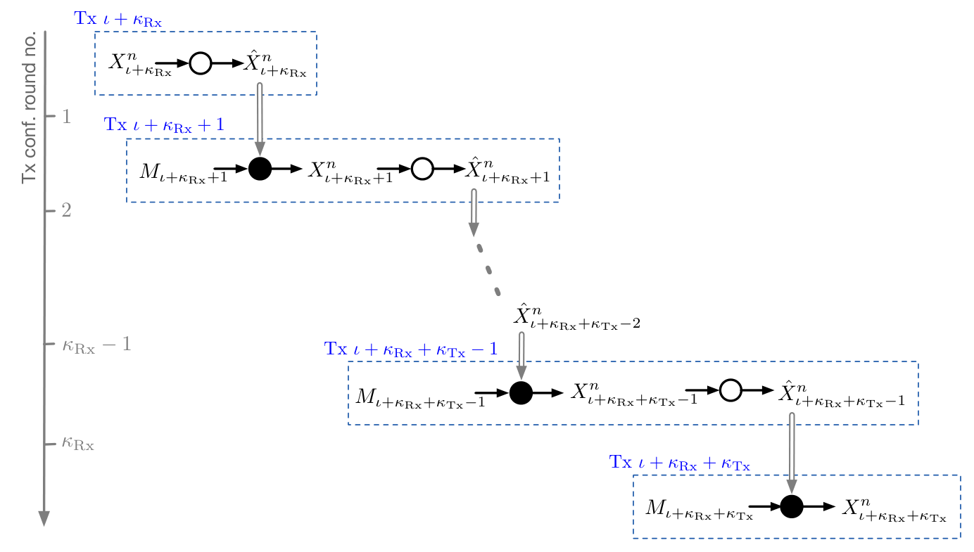
    Fig. 8: Group 2: Tx dirty paper coding from left to right. The dark circles represent dirty paper channel encoders, and the white circles represent vector Gaussian quantisers. Top-down arrows represent communications of quantised input signals over the Tx-conferencing links to right-neighbours.

    To facilitate dirty-paper coding at Tx ι+κRx+1{\iota}+{\kappa_{\text{Rx}}}+1 (the first transmitter in group 2), Tx ι+κRx{\iota}+{\kappa_{\text{Rx}}} (the last transmitter in group 1) quantises its inputs signal Xι+κRxnX_{{\iota}+{\kappa_{\text{Rx}}}}^{n} using a rate-12​log⁡(1+P)\frac{1}{2}\log(1+P) quantiser. It sends the quantisation message to this Tx ι+κRx+1{\iota}+{\kappa_{\text{Rx}}}+1.

    Tx ι+κRx+1{\iota}+{\kappa_{\text{Rx}}}+1 reconstructs the quantised inputs X^ι+κRxn\hat{X}_{{\iota}+{\kappa_{\text{Rx}}}}^{n} and encodes its source message MkM_{k} using a power PP dirty-paper code that eliminates interference αι+κRx+1​X^ι+κRxn\alpha_{{\iota}+{\kappa_{\text{Rx}}}+1}\hat{X}_{{\iota}+{\kappa_{\text{Rx}}}}^{n}.

    Tx ι+κRx+1{\iota}+{\kappa_{\text{Rx}}}+1 also quantises its produced inputs Xι+κRx+1nX_{{\iota}+{\kappa_{\text{Rx}}}+1}^{n} using a rate-12​log⁡(1+P)\frac{1}{2}\log(1+P) quantiser, and sends the quantisation message to Tx ι+κRx+2{\iota}+{\kappa_{\text{Rx}}}+2 (its right-neighbour).

    Rx ι+κRx+1{\iota}+{\kappa_{\text{Rx}}}+1 decodes source message Mι+κRx+1M_{{\iota}+{\kappa_{\text{Rx}}}+1} by applying dirty-paper decoding to its outputs

    Yι+κRx+1n=αι+κRx+1​Xι+κRxn+Xι+κRx+1n+Zι+κRx+1n.Y_{{\iota}+{\kappa_{\text{Rx}}}+1}^{n}=\alpha_{{\iota}+{\kappa_{\text{Rx}}}+1}{X}_{{\iota}+{\kappa_{\text{Rx}}}}^{n}+{X}^{n}_{{\iota}+{\kappa_{\text{Rx}}}+1}+{Z}^{n}_{{\iota}+{\kappa_{\text{Rx}}}+1}.

    Notice that αι+κRx+1​X^ι+κRxn−αι+κRx+1​Xι+κRxn\alpha_{{\iota}+{\kappa_{\text{Rx}}}+1}\hat{X}_{{\iota}+{\kappa_{\text{Rx}}}}^{n}-\alpha_{{\iota}+{\kappa_{\text{Rx}}}+1}{X}_{{\iota}+{\kappa_{\text{Rx}}}}^{n} has variance close to n​αι+κRx+12​PP+1n\alpha_{{\iota}+{\kappa_{\text{Rx}}}+1}^{2}\frac{P}{P+1} and thus for P≫1P\gg 1 the dirty-paper code precancels the predominant part of the interfering signal αι+κRx+1​Xι+κRxn\alpha_{{\iota}+{\kappa_{\text{Rx}}}+1}{X}_{{\iota}+{\kappa_{\text{Rx}}}}^{n}

    The procedure is repeated for transmitters and receivers k=ι+κRx+2,…,ι+κRx+κTxk={\iota}+{\kappa_{\text{Rx}}}+2,\ldots,{\iota}+{\kappa_{\text{Rx}}}+{\kappa_{\text{Tx}}}. Each such Tx kk performs the following three steps:

    1. 1.

      Using the conferencing message from Tx k−1k-1, it reconstructs the quantised signal X^k−1n\hat{X}_{k-1}^{n}.

    2. 2.

      It encodes and transmits its source message MkM_{k} using a power-PP dirty-paper code that eliminates interference αk​X^k−1n\alpha_{k}\hat{X}_{k-1}^{n}.

    3. 3.

      It quantises its input signals XknX_{k}^{n} with a rate-12​log⁡(1+P)\frac{1}{2}\log(1+P) quantiser and sends the produced quantisation message over the conferencing link to Tx k+1k+1.

      Tx ι+κRx+κTx{\iota}+\kappa_{\textnormal{Rx}}+{\kappa_{\text{Tx}}} (the last transmitter in group 𝒢2{\mathcal{G}}_{2}) sends no conferencing message; it skips step 3.

    Each corresponding Rx kk decodes its desired source message MkM_{k} using dirty-paper decoding based on its outputs YknY_{k}^{n}.

    Notice that the described scheme requires only left-to-right Tx-conferencing; no right-to-left Tx-conferencing and no Rx-conferencing. Also, Tx ι+κRx+j{\iota}+{\kappa_{\text{Rx}}}+j, (the jj-th transmitter of group 𝒢2{\mathcal{G}}_{2}), for j∈{1,…,κTx−1}j\in\{1,\ldots,{\kappa_{\text{Tx}}}-1\}, has to wait until it obtains the Tx-conferencing message from its left-neighbour before it can perform above three steps. It can thus send its own Tx-conferencing message to its right-neighbour only in Tx-conferencing round j+1j+1.

    Finally, as we show in detail in Appendix A-B, through a careful design of the vector-quantisers and the dirty-paper codes and when P≫1P\gg 1, the predominant part of the interference αk​Xk−1n\alpha_{k}X_{k-1}^{n} experienced at Rx kk can be precanceled. As a consequence, source messages Mι+κRx+1,…,Mι+κRx+κTxM_{{\iota}+{\kappa_{\text{Rx}}}+1},\ldots,M_{{\iota}+{\kappa_{\text{Rx}}}+{\kappa_{\text{Tx}}}} can be decoded with vanishingly small probability of error as n→∞n\to\infty, whenever (see also Lemma 2 in Appendix A-B)

    Rk<12​log⁡(1+P1+αk2​PP+1),∀k∈𝒢2R_{k}<\frac{1}{2}\log\left(1+\frac{P}{1+\alpha_{k}^{2}\frac{P}{P+1}}\right),\qquad\forall k\in{\mathcal{G}}_{2} (35)

    and

    RTx>12​log⁡(1+P).R_{\textnormal{Tx}}>\frac{1}{2}\log(1+{P}). (36)

Source messages in groups 1 and 2 were transmitted over the “direct” links from a Tx kk to its corresponding Rx kk. The “diagonal” links from a Tx kk to its right-neighbouring Rx k+1k+1 only carried interference that had to be mitigated. In contrast, source messages in groups 3 and 4 are transmitted over the “diagonal” links, whereas the “direct” links carry interference that has to be mitigated. Without conferencing, there exists no desired communication path over the diagonal links, since the source message desired by Rx kk is a priori unknown at its left-neighbour Tx k−1k-1. Setting up such a path requires concatenating the diagonal link from Tx k−1k-1 to Rx kk with a preceding right-to-left Tx-conferencing from Tx kk to Tx k−1k-1 or a subsequent right-to-left Rx-conferencing from Rx kk to Rx k−1k-1, see (44) and (38) ahead.

We now describe transmission of messages in group 4, follows by transmission of messages in group 3.

  • •

    Group 4 (successive interference cancellation from right to left): The fourth group of messages,

    {Mι+β−κRx−1Rx}∪{Mk:k∈𝒢4}\big\{M^{\textnormal{Rx}}_{{\iota}+\beta-{\kappa_{\text{Rx}}}-1}\big\}\cup\big\{M_{k}:k\in{\mathcal{G}}_{4}\big\} (37)

    with

    𝒢4:={ι+β−κRx,…,ι+β−2},{\mathcal{G}}_{4}:=\big\{{\iota}+\beta-{\kappa_{\text{Rx}}},\ldots,{\iota}+\beta-2\},

    is communicated using point-to-point channel codes with right-to-left successive interference cancellation at the decoders. (See Appendix A-C for more technical details.)

    Specifically, each source message MkM_{k}55 5 For ease of notation, in the following paragraph we write simply Mι+β−κRx−1M_{{\iota}+\beta-{\kappa_{\text{Rx}}}-1} for Mι+β−κRx−1RxM_{{\iota}+\beta-{\kappa_{\text{Rx}}}-1}^{\textnormal{Rx}} is sent over the following communication path:

    Tx​k⟶Rx​k+1⟶Rx​k.\textnormal{Tx}~k\;\longrightarrow\;\textnormal{Rx}~{k+1}\;\longrightarrow\;\textnormal{Rx}~k. (38)

    Each Tx k∈𝒢4k\in{\mathcal{G}}_{4} uses a Gaussian point-to-point code of power PP to transmit its source message MkM_{k}.

    Rx ι+β−1{\iota}+\beta-1 (the last receiver in the subnet) observes channel outputs

    Yι+β−1n=αι+β−1​Xι+β−2n​(Mι+β−2)+Zι+β−1n,Y_{{\iota}+\beta-1}^{n}=\alpha_{{\iota}+\beta-1}X_{{\iota}+\beta-2}^{n}(M_{{\iota}+\beta-2})+Z_{{\iota}+\beta-1}^{n}, (39)

    because we silenced its corresponding Tx ι+β−1{{\iota}+\beta-1}. It decodes source message Mι+β−2M_{{{\iota}+\beta-2}} from these channel outputs and describes the decoded message M^ι+β−2\hat{M}_{{\iota}+\beta-2} over the conferencing link to Rx ι+β−2{{\iota}+\beta-2} (its immediate left-neighbour).

    Rx ι+β−2{{\iota}+\beta-2} declares the obtained conferencing message M^ι+β−2\hat{M}_{{\iota}+\beta-2} as its guess of Mι+β−2{M}_{{\iota}+\beta-2}. It further uses the conferencing message to reconstruct Xι+β−2n​(M^ι+β−2)X_{{\iota}+\beta-2}^{n}(\hat{M}_{{\iota}+\beta-2}) and forms

    Y^ι+β−2n=Yι+β−2n−Xι+β−2n​(M^ι+β−2).\hat{Y}_{{\iota}+\beta-2}^{n}={Y}_{{\iota}+\beta-2}^{n}-X_{{\iota}+\beta-2}^{n}(\hat{M}_{{\iota}+\beta-2}).

    Rx ι+β−2{\iota}+\beta-2 finally decodes source message Mι+β−3M_{{\iota}+\beta-3} from this difference and describes M^ι+β−3\hat{M}_{{\iota}+\beta-3} over the conferencing link to Rx ι+β−3{\iota}+\beta-3.

    Whenever M^ι+β−2=Mι+β−2\hat{M}_{{\iota}+\beta-2}={M}_{{\iota}+\beta-2},

    Y^ι+β−2n=αι+β−2​Xι+β−3n​(Mι+β−3)+Zι+β−2n,\hat{Y}_{{\iota}+\beta-2}^{n}=\alpha_{{\iota}+\beta-2}X_{{\iota}+\beta-3}^{n}(M_{{\iota}+\beta-3})+Z_{{\iota}+\beta-2}^{n}, (40)

    and Rx ι+β−2{\iota}+\beta-2 decodes source message Mι+β−3M_{{\iota}+\beta-3} based on an interference-free signal.

    The described procedure is repeated for receivers k=ι+β−3,…,ι+β−κRx−1k={\iota}+\beta-3,\ldots,{\iota}+\beta-{\kappa_{\text{Rx}}}-1 in decreasing order. Specifically, each such Rx kk performs four steps:

    1. 1.

      Using the conferencing message M^k\hat{M}_{k} from Rx k+1k+1, it reconstructs the “interference” Xkn​(M^k)X_{k}^{n}(\hat{M}_{k}).

    2. 2.

      It forms Y^kn:=Ykn−Xkn​(M^k)\hat{Y}_{k}^{n}:=Y_{k}^{n}-{X}_{k}^{n}(\hat{M}_{k}) and decodes source message Mk−1M_{k-1} based on this difference.

    3. 3.

      It sends the decoded source message M^k−1\hat{M}_{k-1} over the conferencing link to Rx k−1k-1.

    4. 4.

      It declares M^k\hat{M}_{k} as its guess of source message MkM_{k}.

    Notice that the described scheme requires only right-to-left Rx-conferencing; no left-to-right Rx-conferencing nor Tx-conferencing. Rx ι+β−1{\iota}+\beta-1 (the last receiver in the subnet) sends its conferencing message M^ι+β−2\hat{M}_{{\iota}+\beta-2} in the first Rx-conferencing round. For each j∈{2,…,κRx}j\in\{2,\ldots,{\kappa_{\text{Rx}}}\}, Rx ι+β−j{\iota}+\beta-j (the jj-th right-most receiver in the subnet) has to wait until it obtains the conferencing message from its right-neighbour before it can start performing above four steps. It can thus send its own conferencing message M^ι+β−j−1\hat{M}_{{\iota}+\beta-j-1} only in Rx-conferencing round jj.

    Finally, we notice that if Rx k+2k+2’s decoding was successful, i.e., M^k+1=Mk+1\hat{M}_{k+1}={M}_{k+1}, then X^k+1n=Xk+1n\hat{X}_{k+1}^{n}=X_{k+1}^{n} and Y^k+1n=αk+1​Xkn+Zk+1n\hat{Y}_{k+1}^{n}=\alpha_{k+1}X_{k}^{n}+Z_{k+1}^{n}, and Rx k+1k+1 can thus decode source message MkM_{k} based on an interference-free signal.

    Consequently, source messages Mι+β−κRx−1Rx,Mι+β−κRx,…,Mι+β−2M_{{\iota}+\beta-{\kappa_{\text{Rx}}}-1}^{\textnormal{Rx}},M_{{\iota}+\beta-{\kappa_{\text{Rx}}}},\ldots,M_{{\iota}+\beta-2} can be decoded with vanishingly small probability of error as n→∞n\to\infty, whenever

    Rk<12​log⁡(1+αk+12​P),k∈𝒢4,R_{k}<\frac{1}{2}\log(1+\alpha_{k+1}^{2}P),\qquad k\in{\mathcal{G}}_{4}, (41a)
    Rι+β−κRx−1Rx<12​log⁡(1+αι+β−κRx2​P),R_{{\iota}+\beta-{\kappa_{\text{Rx}}}-1}^{\textnormal{Rx}}<\frac{1}{2}\log(1+\alpha_{{\iota}+\beta-{\kappa_{\text{Rx}}}}^{2}P), (41b)

    and

    RRx>max⁡{Rι+β−κRx−1Rx,Rι+β−κRx,…,Rι+β−2}.R_{\textnormal{Rx}}>\max\Big\{R_{{\iota}+\beta-{\kappa_{\text{Rx}}}-1}^{\textnormal{Rx}},\ R_{{\iota}+\beta-{\kappa_{\text{Rx}}}},\ \ldots,R_{{\iota}+\beta-2}\Big\}. (42)
  • •

    Group 3 (dirty paper coding from right to left): The third group of messages

    {Mk:k∈𝒢3}∪{Mι+β−κRx−1Tx}\big\{M_{k}:k\in{\mathcal{G}}_{3}\big\}\cup\big\{M^{\textnormal{Tx}}_{{\iota}+\beta-{\kappa_{\text{Rx}}}-1}\big\} (43)

    with

    𝒢3:={ι+β−κRx−κTx,…,ι+β−κRx−2},{\mathcal{G}}_{3}:=\big\{{\iota}+\beta-{\kappa_{\text{Rx}}}-{\kappa_{\text{Tx}}},\ldots,{\iota}+\beta-{\kappa_{\text{Rx}}}-2\big\},

    uses dirty paper coding to mitigate the interference from the right. The desired communication path of a message MkM_{k} is

    Tx​k⟶Tx​k−1⟶Rx​k\textnormal{Tx}~k\;\longrightarrow\;\textnormal{Tx}~k-1\;\longrightarrow\;\textnormal{Rx}~k (44)

    and thus involves Tx-conferencing from right-to-left. More specifically, Tx kk prepares a transmit signal Xk−1nX_{k-1}^{n} that encodes message MkM_{k}. It then describes it over the conferencing link to Tx k−1k-1, which will transmit this signal.

    For simplicity, we temporarily fix k=ι+β−κRx−1k={\iota}+\beta-{\kappa_{\text{Rx}}}-1. In the previous subsection we described how Tx kk (the special transmitter of Figure 6), generated its input signal XknX_{k}^{n} in function of MkRxM_{k}^{\textnormal{Rx}}. Tx kk now also encodes its second message MkTxM_{k}^{\textnormal{Tx}} using a dirty-paper code of power αk2​P2P+1\alpha_{k}^{2}\frac{P^{2}}{P+1} that mitigates its own input signal XknX_{k}^{n}. Denote the produced dirty-paper sequence by ΨDPC,k​(MkRx)\Psi_{\textnormal{DPC},k}\big(M_{k}^{\textnormal{Rx}}\big).

    Tx kk quantises a scaled version of the dirty-paper sequence,

    Φkn:=P+1P​ΨDPC,k​(MkRx)\Phi_{k}^{n}:=\frac{P+1}{P}\Psi_{\textnormal{DPC},k}\big(M_{k}^{\textnormal{Rx}}\big)

    using a rate-12​log⁡(1+P)\frac{1}{2}\log(1+P) quantiser and sends the resulting quantisation message over the conferencing link to Tx k−1k-1 (its left neighbour).

    Tx k−1k-1 reconstructs the quantised sequence Φ^kn\hat{\Phi}_{k}^{n} and transmits

    Xk−1n=αk−1​Φ^knX_{k-1}^{n}=\alpha_{k}^{-1}\hat{\Phi}_{k}^{n}

    over the interference network.

    Rx kk decodes source message MkTxM_{k}^{\textnormal{Tx}} by applying dirty-paper decoding to its outputs YknY_{k}^{n}.

    Notice that if there was no quantisation error,

    Δkn:=Φ^kn−Φkn=0,\Delta_{k}^{n}:=\hat{\Phi}_{k}^{n}-\Phi_{k}^{n}=0, (45)

    then Rx kk would observe outputs

    Ykn=ΨDPC,k​(MkRx)+Xkn+Zkn.Y_{k}^{n}=\Psi_{\textnormal{DPC},k}\big(M_{k}^{\textnormal{Rx}}\big)+X_{k^{n}}+Z_{k}^{n}.

    In this case, since the applied dirty-paper code precancels the “interference” XknX_{k}^{n}, source message MkM_{k} could be transmitted with the same rates as over an interference-free channel.

    Now, zero quantization error (45) is very unlikely. However, when the quantiser is chosen as in Appendix A-D, the normalized variance Var​[1n​Δkn]\textnormal{Var}\big[\frac{1}{n}\Delta_{k}^{n}\big] approaches αk2​1P+1\alpha_{k}^{2}\frac{1}{P+1} and is bounded in PP. Treating the quantisation Δkn\Delta_{k}^{n} simply as an additional noise, will thus not degrade the prelog rate of the source message MkM_{k}. (See Appendix A-D for a more detailed analysis.)

    Let now k=ι+β−κRx−2k={\iota}+\beta-{\kappa_{\text{Rx}}}-2, one less than before.

    Tx kk (which before was Tx k−1k-1) also prepares the transmit signal of its left-neighbour. Specifically, Tx kk encodes its own source message MkM_{k} using a dirty-paper code of power αk2​P2P+1\alpha_{k}^{2}\frac{P^{2}}{P+1} that mitigates its own input signal XknX_{k}^{n}. Let ΨDPC,kn​(Mk)\Psi_{\textnormal{DPC},k}^{n}(M_{k}) denote the produced dirty-paper sequence. Tx kk applies a rate-12​log⁡(1+P)\frac{1}{2}\log(1+P) quantiser to the scaled sequence

    Φkn:=P+1P​ΨDPC,kn​(Mk)\Phi_{k}^{n}:=\frac{P+1}{P}\Psi_{\textnormal{DPC},{k}}^{n}(M_{k})

    and sends the resulting quantisation message to Tx k−1k-1.

    This process is repeated for transmitters and receivers k=ι+β−κRx−3,…,ι+β−κRx−κTxk={\iota}+\beta-{\kappa_{\text{Rx}}}-3,\ldots,{\iota}+\beta-{\kappa_{\text{Rx}}}-{\kappa_{\text{Tx}}} in decreasing order. Each such Tx kk performs the following four steps:66 6 See Appendix A-D for more technical details.

    1. 1.

      Using the conferencing message from Tx k+1k+1, it reconstructs the quantised signal Φ^k+1n\hat{\Phi}_{k+1}^{n}.

    2. 2.

      It transmits Xkn=αk+1−1​Φ^k+1nX_{k}^{n}=\alpha_{k+1}^{-1}\hat{\Phi}_{k+1}^{n} over the network.

    3. 3.

      It encodes source message MkM_{k} using dirty-paper coding of power αk2​P2P+1\alpha_{k}^{2}\frac{P^{2}}{P+1} that mitigates its own inputs XknX_{k}^{n}. It then forms Φkn=P+1P​ΨDPC,kn​(Mk){\Phi}_{k}^{n}=\frac{P+1}{P}\Psi_{\textnormal{DPC},k}^{n}(M_{k}), where ΨDPC,kn​(Mk)\Psi_{\textnormal{DPC},k}^{n}(M_{k}) denotes the produced dirty-paper sequence.

    4. 4.

      It quantises Φkn{\Phi}_{k}^{n} using a rate-12​log⁡(1+P)\frac{1}{2}\log(1+P) quantiser and sends the resulting quantisation bits over the conferencing link to Tx k−1k-1.

    Tx ι+κRx+κTx+1{\iota}+{\kappa_{\text{Rx}}}+{\kappa_{\text{Tx}}}+1 (the left-most transmitter only performs steps 1) and 4), but prepares and sends no conferencing message.

    Each receiver applies dirty-paper decoding to decode its desired message MkM_{k} based on its outputs YknY_{k}^{n}.

    Notice that the described scheme requires right-to-left Tx-conferencing; no left-to-right Tx-conferencing or Rx-conferencing are needed. Special Tx ι+κRx+2​κTx+1{\iota}+{\kappa_{\text{Rx}}}+2{\kappa_{\text{Tx}}}+1 sends its conferencing message in Tx-conferencing round 11. Each Tx ι+β−κRx−ȷ{\iota}+\beta-{\kappa_{\text{Rx}}}-\char 17\relax, for j∈{2,…,κTx−1}j\in\{2,\ldots,{\kappa_{\text{Tx}}}-1\} can send its conferencing message only after receiving the conferencing message from its right-neighbour. Tx ι+β−κRx−ȷ{\iota}+\beta-{\kappa_{\text{Rx}}}-\char 17\relax can thus send its conferencing message only in Tx-conferencing round j+1j+1.

    Finally, as we show in detail in Appendix A-D, through a careful design of the quantisers and the dirty-paper codes, source messages Mι+β−κRx−κTx,…,Mι+β−κRx−1TxM_{{\iota}+\beta-{\kappa_{\text{Rx}}}-{\kappa_{\text{Tx}}}},\ldots,M_{{\iota}+\beta-{\kappa_{\text{Rx}}}-1}^{\textnormal{Tx}} can be decoded with vanishingly small probability of error as n→∞n\to\infty, whenever

    Rk<12​log⁡(1+αk2​P2P+11+αk2​PP+1),k∈𝒢3,\displaystyle R_{k}<\frac{1}{2}\log\left(1+\frac{\alpha_{k}^{2}\frac{P^{2}}{P+1}}{1+\alpha_{k}^{2}\frac{P}{P+1}}\right),\hskip 28.45274ptk\in\mathcal{G}_{3}, (46a)
    Rι+β−κRx−1Tx<12​log⁡(1+P2P+1​αι+β−κRx−121+PP+1​αι+β−κRx−12)R_{{\iota}+\beta-{\kappa_{\text{Rx}}}-1}^{\textnormal{Tx}}<\frac{1}{2}\log\left(1+\frac{\frac{P^{2}}{P+1}\alpha_{{\iota}+\beta-{\kappa_{\text{Rx}}}-1}^{2}}{1+\frac{P}{P+1}\alpha_{{\iota}+\beta-{\kappa_{\text{Rx}}}-1}^{2}}\right) (46b)

    and

    RTx>12​log⁡(1+P).R_{\textnormal{Tx}}>\frac{1}{2}\log(1+{P}). (47)

IV-C Tx-Conferencing in Period 2

If in the previous subsection IV-B we set everywhere κRx=0\kappa_{\textnormal{Rx}}=0, and hence 𝒢1=𝒢4=∅\mathcal{G}_{1}=\mathcal{G}_{4}=\emptyset, we obtain our scheme for period 2 in case of Tx-conferencing only. In this case, there is no need for a message Mι+κTx+2​κRx+1Rx{M}_{{\iota}+{\kappa_{\text{Tx}}}+2{\kappa_{\text{Rx}}}+1}^{\textnormal{Rx}} and we can simply set Mι+κTx+2​κRx+1Tx=Mι+κTx+2​κRx+1{M}_{{\iota}+{\kappa_{\text{Tx}}}+2{\kappa_{\text{Rx}}}+1}^{\textnormal{Tx}}={M}_{{\iota}+{\kappa_{\text{Tx}}}+2{\kappa_{\text{Rx}}}+1}.

IV-D No Conferencing in Period 3

We silence all odd transmitters. This splits the network into a set of ⌈K2⌉\lceil\frac{K}{2}\rceil parallel Gaussian point-to-point channels. We use optimal point-to-point codes over these channels.

IV-E Analysis

IV-E1 Analysis of Period 1

As argued in (32), (35), (41) and (46) (see also lemmas 1–4), in each subnet we can transmit 2​κTx+2​κTx+12{\kappa_{\text{Tx}}}+2{\kappa_{\text{Tx}}}+1 (sub)messages each of MG 1. Thus, over the entire network which consists of γ\gamma subnets, our scheme achieves a MG of

γ⁡(2​κTx+2​κRx+1),\gamma(2{\kappa_{\text{Tx}}}+2\kappa_{\textnormal{Rx}}+1), (48)

and a per-user MG of

𝖲period1=2​κTx+2​κRx+12​κTx+2​κRx+2.{\sf{S}}_{\textnormal{period1}}=\frac{2{\kappa_{\text{Tx}}}+2\kappa_{\textnormal{Rx}}+1}{2{\kappa_{\text{Tx}}}+2\kappa_{\textnormal{Rx}}+2}. (49)

We now analyse the communication over the conferencing links. We have for each subnet g=0,…,γ−1g=0,\ldots,\gamma-1 (see lemmas 1–4),

  • •

    Only the κTx{\kappa_{\text{Tx}}} consecutive transmitters ι+g​β+κRx,…,ι+g​β+κRx+κTx−1{\iota}+g\beta+{\kappa_{\text{Rx}}},\ldots,{\iota}+g\beta+{\kappa_{\text{Rx}}}+{\kappa_{\text{Tx}}}-1 send conferencing messages to their right-neighbours. Each of these messages corresponds to a decoded source message. Since we transmit all source messages at rates below 12​log⁡(1+P)\frac{1}{2}\log(1+P), also the rates of the conferencing messages do not exceed 12​log⁡(1+P)\frac{1}{2}\log(1+P).

  • •

    Only the κTx{\kappa_{\text{Tx}}} consecutive transmitters ι+(g+1)​β−κRx−κTx,…,ι+(g+1)​β−κRx−1{\iota}+(g+1)\beta-{\kappa_{\text{Rx}}}-{\kappa_{\text{Tx}}},\ldots,{\iota}+(g+1)\beta-{\kappa_{\text{Rx}}}-1 send conferencing messages to their left-neighbours. Each of these messages corresponds to a decoded source message. Since we transmit all source messages at rates below 12​log⁡(1+P)\frac{1}{2}\log(1+P), also the rates of the conferencing messages do not exceed 12​log⁡(1+P)\frac{1}{2}\log(1+P).

  • •

    Only the κRx{\kappa_{\text{Rx}}} consecutive receivers ι+g​β,…,ι+g​β+κRx−1{\iota}+g\beta,\ldots,{\iota}+g\beta+{\kappa_{\text{Rx}}}-1 send conferencing messages to their right-neighbours. Each of these messages corresponds to a rate-12​log⁡(1+P)\frac{1}{2}\log(1+P) quantisation message.77 7 More precisely, the rate should be slightly larger than 12​log⁡(1+P)\frac{1}{2}\log(1+P). Through standard continuity considerations one can show that this does not change the set of achievable rates. It is thus a minor technicality, which we ignore.

  • •

    Only the κRx{\kappa_{\text{Rx}}} consecutive receivers ι+(g+1)​β−κRx,…,ι+(g+1)​β−1{\iota}+(g+1)\beta-{\kappa_{\text{Rx}}},\ldots,{\iota}+(g+1)\beta-1 send conferencing messages to their left-neighbours. Each of these messages corresponds to a rate-12​log⁡(1+P)\frac{1}{2}\log(1+P) quantisation message.

We conclude that each Tx-conferencing link is used a κTx2​κTx+2​κRx+2\frac{{\kappa_{\text{Tx}}}}{2{\kappa_{\text{Tx}}}+2{\kappa_{\text{Rx}}}+2}-th of the time and at a total rate not exceeding

μTx,Period1=κTx2​κTx+2​κRx+2⋅12​log⁡(1+P).\mu_{\textnormal{Tx},\textnormal{Period1}}=\frac{{\kappa_{\text{Tx}}}}{2{\kappa_{\text{Tx}}}+2{\kappa_{\text{Rx}}}+2}\cdot\frac{1}{2}\log(1+P). (50)

Similarly, each Rx-conferencing link is used a κRx2​κTx+2​κRx+2\frac{{\kappa_{\text{Rx}}}}{2{\kappa_{\text{Tx}}}+2{\kappa_{\text{Rx}}}+2}-th of the time and at a total rate not exceeding

μRx,Period1=κRx2​κTx+2​κRx+2⋅12​log⁡(1+P).\mu_{\textnormal{Rx},\textnormal{Period1}}=\frac{{\kappa_{\text{Rx}}}}{2{\kappa_{\text{Tx}}}+2{\kappa_{\text{Rx}}}+2}\cdot\frac{1}{2}\log(1+P). (51)

IV-E2 Analysis of Period 2

Specializing the findings of the previous section to κRx=0{\kappa_{\text{Rx}}}=0, the per-user MG achieved in period 2 is

𝖲period2=2​κTx+12​κTx+2.{\sf{S}}_{\textnormal{period2}}=\frac{2{\kappa_{\text{Tx}}}+1}{2{\kappa_{\text{Tx}}}+2}. (52)

The tx-conferencing links are used at rate

μTx,Period2=κTx2​κTx+2⋅12​log⁡(1+P),\mu_{\textnormal{Tx},\textnormal{Period2}}=\frac{{\kappa_{\text{Tx}}}}{2{\kappa_{\text{Tx}}}+2}\cdot\frac{1}{2}\log(1+P), (53)

and the rx-conferencing links are not used at all,

μRx,Period2=0.\mu_{\textnormal{Rx},\textnormal{Period2}}=0. (54)

IV-E3 Analysis of Period 3

During the third period the achieved per-user MG is

𝖲period3=12.{\sf{S}}_{\textnormal{period3}}=\frac{1}{2}. (55)

The conferencing links are not used at all,

μTx,Period3\displaystyle\mu_{\textnormal{Tx},\textnormal{Period3}} =\displaystyle= 0\displaystyle 0 (56)
μRx,Period3\displaystyle\mu_{\textnormal{Rx},\textnormal{Period3}} =\displaystyle= 0.\displaystyle 0. (57)

IV-E4 Analysis of Overall Scheme

We first analyse the communication over the conferencing links. Under assumption (25), there is tx-conferencing in periods 1 and 2. Given the length of the periods in (26), and the tx-conferencing rates in periods 1 and 2, (50) and (53), in total each tx-conferencing link is used at rate not exceeding

 N1n​μTx,period1+N2n​μTx,period2\displaystyle\frac{N_{1}}{n}\mu_{\textnormal{Tx},\textnormal{period1}}+\frac{N_{2}}{n}\mu_{\textnormal{Tx},\textnormal{period2}} (58)
=\displaystyle= (N1n⋅κTx2​κTx+2​κRx+2+N2n⋅κTx2​κTx+2)⋅12​log⁡(1+P)\displaystyle\left(\frac{N_{1}}{n}\cdot\frac{{\kappa_{\text{Tx}}}}{2{\kappa_{\text{Tx}}}+2{\kappa_{\text{Rx}}}+2}+\frac{N_{2}}{n}\cdot\frac{{\kappa_{\text{Tx}}}}{2{\kappa_{\text{Tx}}}+2}\right)\cdot\frac{1}{2}\log(1+P)
≤\displaystyle\leq (μRxκRx​(2​κTx+2​κRx+2)​κTx2​κTx+2​κRx+2+(μTxκTx−μRxκRx)​(2​κTx+2)​κTx2​κTx+2)⋅12​log⁡(1+P)\displaystyle\left(\frac{{\mu}_{\textnormal{Rx}}}{{\kappa_{\text{Rx}}}}(2{\kappa_{\text{Tx}}}+2{\kappa_{\text{Rx}}}+2)\frac{{\kappa_{\text{Tx}}}}{2{\kappa_{\text{Tx}}}+2{\kappa_{\text{Rx}}}+2}+\Big(\frac{{\mu}_{\textnormal{Tx}}}{{\kappa_{\text{Tx}}}}-\frac{{\mu}_{\textnormal{Rx}}}{{\kappa_{\text{Rx}}}}\Big)(2{\kappa_{\text{Tx}}}+2)\frac{{\kappa_{\text{Tx}}}}{2{\kappa_{\text{Tx}}}+2}\right)\cdot\frac{1}{2}\log(1+P)
≤\displaystyle\leq μTx⋅12​log⁡(1+P)=RTx.\displaystyle{{\mu}_{\textnormal{Tx}}}\cdot\frac{1}{2}\log(1+P)={R_{\textnormal{Tx}}}.

Our overall scheme thus respects the tx-conferencing rate constraints in (6).

The rx-conferencing links are used only in period 1 at rate not exceeding (51). Thus, considering the length of this period 1 in (26), in total each receiver conferencing link is used at a rate not exceeding

N1n​μRx,period1\displaystyle\frac{N_{1}}{n}\mu_{\textnormal{Rx},\textnormal{period1}} =\displaystyle= N1n⋅κRx2​κTx+2​κRx+2⋅12​log⁡(1+P)\displaystyle\frac{N_{1}}{n}\cdot\frac{{\kappa_{\text{Rx}}}}{2{\kappa_{\text{Tx}}}+2{\kappa_{\text{Rx}}}+2}\cdot\frac{1}{2}\log(1+P) (59)
≤\displaystyle\leq μRxκRx​(2​κTx+2​κRx+2)⋅κRx2​κTx+2​κRx+2⋅12​log⁡(1+P)\displaystyle\frac{{\mu}_{\textnormal{Rx}}}{{\kappa_{\text{Rx}}}}(2{\kappa_{\text{Tx}}}+2{\kappa_{\text{Rx}}}+2)\cdot\frac{{\kappa_{\text{Rx}}}}{2{\kappa_{\text{Tx}}}+2{\kappa_{\text{Rx}}}+2}\cdot\frac{1}{2}\log(1+P)
=\displaystyle= μRx⋅12​log⁡(1+P)=RRx.\displaystyle{{\mu}_{\textnormal{Rx}}}\cdot\frac{1}{2}\log(1+P)={R_{\textnormal{Rx}}}.

Our overall scheme thus also respects the rx-conferencing rate constraints in (9).

We now analyse the per-user MG achieved by our overall scheme. It is given by

𝖲=N1n​𝖲period1+N2n​𝖲period2+N3n​𝖲period3.{\sf{S}}=\frac{N_{1}}{n}{\sf{S}}_{\textnormal{period1}}+\frac{N_{2}}{n}{\sf{S}}_{\textnormal{period2}}+\frac{N_{3}}{n}{\sf{S}}_{\textnormal{period3}}. (60)

To evaluate this expression, we distinguish three cases:

  1. 1.

    When

    1≤μRxκRx​(2​κTx+2​κRx+2),1\leq\frac{{\mu}_{\textnormal{Rx}}}{{\kappa_{\text{Rx}}}}(2{\kappa_{\text{Tx}}}+2{\kappa_{\text{Rx}}}+2), (61)

    then N1=nN_{1}=n and periods 2 and 3 don’t exist. In this case,

    𝖲=𝖲period1=2​κTx+2​κRx+12​κTx+2​κRx+2.{\sf{S}}={\sf{S}}_{\textnormal{period1}}=\frac{2{\kappa_{\text{Tx}}}+2{\kappa_{\text{Rx}}}+1}{2{\kappa_{\text{Tx}}}+2{\kappa_{\text{Rx}}}+2}. (62)
  2. 2.

    When 1>μRxκRx​(2​κTx+2​κRx+2)1>\frac{{\mu}_{\textnormal{Rx}}}{{\kappa_{\text{Rx}}}}(2{\kappa_{\text{Tx}}}+2{\kappa_{\text{Rx}}}+2) and

    1<μRxκRx​(2​κTx+2​κRx+2)+(μTxκTx−μRxκRx)​(2​κTx+2)=2​μTx+2​μRx+2​μTxκTx,\displaystyle 1<\frac{{\mu}_{\textnormal{Rx}}}{{\kappa_{\text{Rx}}}}(2{\kappa_{\text{Tx}}}+2{\kappa_{\text{Rx}}}+2)+\Big(\frac{{\mu}_{\textnormal{Tx}}}{{\kappa_{\text{Tx}}}}-\frac{{\mu}_{\textnormal{Rx}}}{{\kappa_{\text{Rx}}}}\Big)(2{\kappa_{\text{Tx}}}+2)=2{\mu}_{\textnormal{Tx}}+2{\mu}_{\textnormal{Rx}}+2\frac{{\mu}_{\textnormal{Tx}}}{{\kappa_{\text{Tx}}}}, (63)

    then N1=n​μRxκRx​(2​κTx+2​κRx+2)N_{1}=n\frac{{\mu}_{\textnormal{Rx}}}{{\kappa_{\text{Rx}}}}(2{\kappa_{\text{Tx}}}+2{\kappa_{\text{Rx}}}+2), N2=n−N1N_{2}=n-N_{1} and N3=0N_{3}=0, i.e., period 3 does not exist. In this case,

    𝖲\displaystyle{\sf{S}} =\displaystyle= N1n​𝖲period1+(1−N1n)​𝖲period2\displaystyle\frac{N_{1}}{n}{\sf{S}}_{\textnormal{period1}}+\Big(1-\frac{N_{1}}{n}\Big){\sf{S}}_{\textnormal{period2}} (64)
    =\displaystyle= μRxκRx​(2​κTx+2​κRx+2)⋅2​κTx+2​κRx+12​κTx+2​κRx+2+(1−μRxκRx​(2​κTx+2​κRx+2))​2​κTx+12​κTx+2\displaystyle\frac{{\mu}_{\textnormal{Rx}}}{{\kappa_{\text{Rx}}}}(2{\kappa_{\text{Tx}}}+2{\kappa_{\text{Rx}}}+2)\cdot\frac{2{\kappa_{\text{Tx}}}+2{\kappa_{\text{Rx}}}+1}{2{\kappa_{\text{Tx}}}+2{\kappa_{\text{Rx}}}+2}+\left(1-\frac{{\mu}_{\textnormal{Rx}}}{{\kappa_{\text{Rx}}}}(2{\kappa_{\text{Tx}}}+2{\kappa_{\text{Rx}}}+2)\right)\frac{2{\kappa_{\text{Tx}}}+1}{2{\kappa_{\text{Tx}}}+2}
    =\displaystyle= 2​κTx+12​κTx+2+μRxκRx​(2​κTx+2​κRx+2)​(2​κTx+2​κRx+12​κTx+2​κRx+2−2​κTx+12​κTx+2)\displaystyle\frac{2{\kappa_{\text{Tx}}}+1}{2{\kappa_{\text{Tx}}}+2}+\frac{{\mu}_{\textnormal{Rx}}}{{\kappa_{\text{Rx}}}}(2{\kappa_{\text{Tx}}}+2{\kappa_{\text{Rx}}}+2)\left(\frac{2{\kappa_{\text{Tx}}}+2{\kappa_{\text{Rx}}}+1}{2{\kappa_{\text{Tx}}}+2{\kappa_{\text{Rx}}}+2}-\frac{2{\kappa_{\text{Tx}}}+1}{2{\kappa_{\text{Tx}}}+2}\right)
    =\displaystyle= 2​κTx+1+2​μRx2​κTx+2.\displaystyle\frac{2{\kappa_{\text{Tx}}}+1+2{\mu}_{\textnormal{Rx}}}{2{\kappa_{\text{Tx}}}+2}.
  3. 3.

    When

    1>2​μTx+2​μRx+2​μTxκTx,1>2{\mu}_{\textnormal{Tx}}+2{\mu}_{\textnormal{Rx}}+2\frac{{\mu}_{\textnormal{Tx}}}{{\kappa_{\text{Tx}}}},

    then N1=n​μRxκRx​(2​κTx+2​κRx+2)N_{1}=n\frac{{\mu}_{\textnormal{Rx}}}{{\kappa_{\text{Rx}}}}(2{\kappa_{\text{Tx}}}+2{\kappa_{\text{Rx}}}+2), N2=n⁡(μTxκTx−μRxκRx)​(2​κTx+2)N_{2}=n\Big(\frac{{\mu}_{\textnormal{Tx}}}{{\kappa_{\text{Tx}}}}-\frac{{\mu}_{\textnormal{Rx}}}{{\kappa_{\text{Rx}}}}\Big)(2{\kappa_{\text{Tx}}}+2) and N3=n−N1−N−2>0N_{3}=n-N_{1}-N-2>0. In this case,

    𝖲\displaystyle{\sf{S}} =\displaystyle= N1n​𝖲period1+N2n​𝖲period2+(1−N1n−N2n)​𝖲period3\displaystyle\frac{N_{1}}{n}{\sf{S}}_{\textnormal{period1}}+\frac{N_{2}}{n}{\sf{S}}_{\textnormal{period2}}+\left(1-\frac{N_{1}}{n}-\frac{N_{2}}{n}\right){\sf{S}}_{\textnormal{period3}} (65)
    =μRxκRx​(2​κTx+2​κRx+2)⋅2​κTx+2​κRx+12​κTx+2​κRx+2+(μTxκTx−μRxκRx)​(2​κTx+2)⋅2​κTx+12​κTx+2\displaystyle=\frac{{\mu}_{\textnormal{Rx}}}{{\kappa_{\text{Rx}}}}(2{\kappa_{\text{Tx}}}+2{\kappa_{\text{Rx}}}+2)\cdot\frac{2{\kappa_{\text{Tx}}}+2{\kappa_{\text{Rx}}}+1}{2{\kappa_{\text{Tx}}}+2{\kappa_{\text{Rx}}}+2}+\Big(\frac{{\mu}_{\textnormal{Tx}}}{{\kappa_{\text{Tx}}}}-\frac{{\mu}_{\textnormal{Rx}}}{{\kappa_{\text{Rx}}}}\Big)(2{\kappa_{\text{Tx}}}+2)\cdot\frac{2{\kappa_{\text{Tx}}}+1}{2{\kappa_{\text{Tx}}}+2}
    +(1−μRxκRx(2κTx+2κRx+2)−(μTxκTx−μRxκRx)(2κTx+2))⋅12\displaystyle+\left(1-\frac{{\mu}_{\textnormal{Rx}}}{{\kappa_{\text{Rx}}}}(2{\kappa_{\text{Tx}}}+2{\kappa_{\text{Rx}}}+2)-\Big(\frac{{\mu}_{\textnormal{Tx}}}{{\kappa_{\text{Tx}}}}-\frac{{\mu}_{\textnormal{Rx}}}{{\kappa_{\text{Rx}}}}\Big)(2{\kappa_{\text{Tx}}}+2)\right)\cdot\frac{1}{2}
    =\displaystyle= 1+2​μTx+2​μRx2.\displaystyle\frac{1+2{\mu}_{\textnormal{Tx}}+2{\mu}_{\textnormal{Rx}}}{2}.

Combining all these findings proves Theorem 2.

V Proof of Theorem 1

Since with an unlimited number of conferencing rounds we cannot do worse than with 𝜿=(κTx,κRx){\boldsymbol{\kappa}}=(\kappa_{\textnormal{Tx}},\kappa_{\textnormal{Rx}}) conferencing rounds, by Theorem 3,

𝖲⁡(𝜿,𝝁)≤𝖲∞​(𝝁)≤2​μTx+2​μRx+12.{\sf{S}}({\boldsymbol{\kappa}},{\boldsymbol{\mu}})\leq{\sf{S}}_{\infty}({\boldsymbol{\mu}})\leq\frac{2{\mu}_{\textnormal{Tx}}+2{\mu}_{\textnormal{Rx}}+1}{2}. (66)

We now prove that also

𝖲⁡(𝜿,𝝁)≤2​κTx+2​κRx+12​κTx+2​κRx+2{\sf{S}}({\boldsymbol{\kappa}},{\boldsymbol{\mu}})\leq\frac{2{\kappa_{\text{Tx}}}+2{\kappa_{\text{Rx}}}+1}{2{\kappa_{\text{Tx}}}+2{\kappa_{\text{Rx}}}+2} (67)

holds. Let us suppose that a genie provides each transmitter the source messages of the κTx{\kappa_{\text{Tx}}} transmitters on its left and right; that is, transmitter kk is given source messages

(Mk−κTx​…​Mk−1)and(Mk+1​…​Mk+κTx).(M_{k-{\kappa_{\text{Tx}}}}\ \ldots\ M_{k-1})\quad\text{and}\quad(M_{k+1}\ \ldots\ M_{k+{\kappa_{\text{Tx}}}}).

Let us also suppose that the genie provides to each receiver the exact channel outputs at the κRx{\kappa_{\text{Rx}}} receivers on its left and right; that is, receiver kk is given

(Yk−κRxn​…​Yk−1n)and(Yk+1n​…​Yk+κRxn).(Y^{n}_{k-{\kappa_{\text{Rx}}}}\ \ldots\ Y^{n}_{k-1})\quad\text{and}\quad(Y^{n}_{k+1}\ \ldots\ Y^{n}_{k+{\kappa_{\text{Rx}}}}).

Lapidoth et al. [31, Cor. 2] established that the per-user MG of this genie-aided problem is given by (2​κTx+2​κRx+1)/(2​κTx+2​κRx+2)(2{\kappa_{\text{Tx}}}+2{\kappa_{\text{Rx}}}+1)/(2{\kappa_{\text{Tx}}}+2{\kappa_{\text{Rx}}}+2). Since the per-user MG of the genie-aided problem cannot be smaller than 𝖲⁡(𝜿,𝝁){\sf{S}}({\boldsymbol{\kappa}},{\boldsymbol{\mu}}) in the problem at hand, we obtain upper bound (67).

We now establish the converse bound (12) for the case μTx=0{\mu}_{\textnormal{Tx}}=0. The other parameters 𝜿=(κTx,κRx){\boldsymbol{\kappa}}=({\kappa_{\text{Tx}}},{\kappa_{\text{Rx}}}) and μRx{\mu}_{\textnormal{Rx}} are arbitrary. By Proposition 1,

𝖲⁡(0,κRx,0,μRx)=𝖲⁡(1,κRx,0,μRx)=⋯.{\sf{S}}(0,{\kappa_{\text{Rx}}},0,{\mu}_{\textnormal{Rx}})={\sf{S}}(1,{\kappa_{\text{Rx}}},0,{\mu}_{\textnormal{Rx}})=\cdots.

The genie-aided arguments in the preceding paragraph remain valid for 𝜿′=(0,κRx){\boldsymbol{\kappa}}^{\prime}=(0,{\kappa_{\text{Rx}}}) and 𝝁′=(0,μRx){\boldsymbol{\mu}}^{\prime}=(0,{\mu}_{\textnormal{Rx}}), so

𝖲⁡(κTx,κRx,0,μRx)=𝖲⁡(0,κRx,0,μRx)≤2​κRx+12​κRx+2,{\sf{S}}({\kappa_{\text{Tx}}},{\kappa_{\text{Rx}}},0,{\mu}_{\textnormal{Rx}})={\sf{S}}(0,{\kappa_{\text{Rx}}},0,{\mu}_{\textnormal{Rx}})\leq\frac{2{\kappa_{\text{Rx}}}+1}{2{\kappa_{\text{Rx}}}+2},

which establishes (12).

The converse bound (13) for μRx=0{\mu}_{\textnormal{Rx}}=0 can be proved in a similar way.

VI Proof of Converse to Theorem 3

We prove the converse bound in (18),

𝖲∞​(𝝁)\displaystyle{\sf{S}}_{\infty}({\boldsymbol{\mu}}) ≤\displaystyle\leq 1+2​μTx+2​μRx2.\displaystyle\frac{1+2\mu_{\textnormal{Tx}}+2\mu_{\textnormal{Rx}}}{2}.

Assume for the moment that KK is even, and let

αmax≜maxk=2,…,K⁡|αk|.\alpha_{\max}\triangleq\max_{k=2,\ldots,K}|\alpha_{k}|. (68)

Define ℐeven\mathcal{I}_{\textnormal{even}} and ℐodd\mathcal{I}_{\textnormal{odd}} to be the sets of indices in {1,…,K}\{1,\ldots,K\} that are even and odd respectively:

ℐeven\displaystyle\mathcal{I}_{\textnormal{even}} ≜\displaystyle\triangleq {k∈{1,…,K}:k​ is even}\displaystyle\big\{k\in\{1,\ldots,K\}\colon k\textnormal{ is even}\big\} (69)
ℐodd\displaystyle\mathcal{I}_{\textnormal{odd}} ≜\displaystyle\triangleq {k∈{1,…,K}:k​ is odd}.\displaystyle\big\{k\in\{1,\ldots,K\}\colon k\textnormal{ is odd}\big\}. (70)

Define further

𝐌even\displaystyle\mathbf{M}_{\textnormal{even}} ≜\displaystyle\triangleq {Mk:k∈ℐeven}\displaystyle\big\{M_{k}\colon k\in\mathcal{I}_{\textnormal{even}}\big\} (71)
𝐌odd\displaystyle\mathbf{M}_{\textnormal{odd}} ≜\displaystyle\triangleq {Mk:k∈ℐodd}\displaystyle\big\{M_{k}\colon k\in\mathcal{I}_{\textnormal{odd}}\big\} (72)
𝐗evenn\displaystyle\mathbf{X}_{\textnormal{even}}^{n} ≜\displaystyle\triangleq {Xkn:k∈ℐeven}\displaystyle\big\{X_{k}^{n}\colon k\in\mathcal{I}_{\textnormal{even}}\big\} (73)
𝐘evenn\displaystyle\mathbf{Y}_{\textnormal{even}}^{n} ≜\displaystyle\triangleq {Ykn:k∈ℐeven}\displaystyle\big\{Y_{k}^{n}\colon k\in\mathcal{I}_{\textnormal{even}}\big\} (74)
𝐘oddn\displaystyle\mathbf{Y}_{\textnormal{odd}}^{n} ≜\displaystyle\triangleq {Ykn:k∈ℐodd}\displaystyle\big\{Y_{k}^{n}\colon k\in\mathcal{I}_{\textnormal{odd}}\big\} (75)
𝐆noises,evenn\displaystyle\mathbf{G}_{\textnormal{noises},\textnormal{even}}^{n} ≜\displaystyle\triangleq (α2​Z1n−Z2n,α4​Z3n−Z4nCLOSE,\displaystyle\bigg(\alpha_{2}Z_{1}^{n}-Z_{2}^{n},\alpha_{4}Z_{3}^{n}-Z_{4}^{n}, (76)
OPENα6​Z5n−Z6n,…,αK​ZK−1n−ZKn)\displaystyle\hskip 28.45274pt\alpha_{6}Z_{5}^{n}-Z_{6}^{n},\ldots,\alpha_{K}Z_{K-1}^{n}-Z_{K}^{n}\bigg)

and

𝐆noises,oddn\displaystyle\mathbf{G}_{\textnormal{noises},\textnormal{odd}}^{n} ≜\displaystyle\triangleq (α3​Z2n−Z3n,α5​Z4n−Z5nCLOSE,\displaystyle\bigg(\alpha_{3}Z_{2}^{n}-Z_{3}^{n},\alpha_{5}Z_{4}^{n}-Z_{5}^{n},
OPENα7​Z6n−Z7n,…,αK−1​ZK−2n−ZK−1n)\displaystyle\hskip 28.45274pt\alpha_{7}Z_{6}^{n}-Z_{7}^{n},\ldots,\alpha_{K-1}Z_{K-2}^{n}-Z_{K-1}^{n}\bigg)

Also, let 𝐔even→odd\mathbf{U}_{\textnormal{even}\to\textnormal{odd}} denote the set of all cooperation messages that are sent from transmitters with even indices to transmitters with odd indices:

𝐔even→odd≜{Uk′→k(1),…,Uk′→k(κTx):k′∈ℐeven,k∈ℐodd}.\mathbf{U}_{\textnormal{even}\to\textnormal{odd}}\triangleq\Big\{U_{k^{\prime}\to k}^{(1)},\ldots,U_{k^{\prime}\to k}^{({\kappa_{\text{Tx}}})}\colon k^{\prime}\in\mathcal{I}_{\textnormal{even}},\;k\in\mathcal{I}_{\textnormal{odd}}\Big\}. (78)

Similarly, let 𝐔odd→even\mathbf{U}_{\textnormal{odd}\to\textnormal{even}} denote the set of all cooperation messages that are sent from transmitters with odd indices to transmitters with even indices:

𝐔odd→even≜{Uk′→k(1),…,Uk′→k(κTx):k′∈ℐodd,k∈ℐeven}.\mathbf{U}_{\textnormal{odd}\to\textnormal{even}}\triangleq\Big\{U_{k^{\prime}\to k}^{(1)},\ldots,U_{k^{\prime}\to k}^{({\kappa_{\text{Tx}}})}\colon k^{\prime}\in\mathcal{I}_{\textnormal{odd}},\;k\in\mathcal{I}_{\textnormal{even}}\Big\}. (79)

In the same way, let 𝐕even→odd\mathbf{V}_{\textnormal{even}\to\textnormal{odd}} denote the set of all cooperation messages that are sent from receivers with even indices to receivers with odd indices,

𝐕even→odd≜{Vk′→k(1),…,Vk′→k(κRx):k′∈ℐeven,k∈ℐodd}.\mathbf{V}_{\textnormal{even}\to\textnormal{odd}}\triangleq\Big\{V_{k^{\prime}\to k}^{(1)},\ldots,V_{k^{\prime}\to k}^{({\kappa_{\text{Rx}}})}\colon k^{\prime}\in\mathcal{I}_{\textnormal{even}},\;k\in\mathcal{I}_{\textnormal{odd}}\Big\}. (80)

and let 𝐕odd→even\mathbf{V}_{\textnormal{odd}\to\textnormal{even}} denote the set of all cooperation messages that are sent from receivers with odd indices to receivers with even indices:

𝐕odd→even≜{Vk′→k(1),…,Vk′→k(κRx):k′∈ℐodd,k∈ℐeven}.\mathbf{V}_{\textnormal{odd}\to\textnormal{even}}\triangleq\Big\{V_{k^{\prime}\to k}^{(1)},\ldots,V_{k^{\prime}\to k}^{({\kappa_{\text{Rx}}})}\colon k^{\prime}\in\mathcal{I}_{\textnormal{odd}},\;k\in\mathcal{I}_{\textnormal{even}}\Big\}. (81)

Our converse proof is based on the following observations:

  • i)

    From 𝐕even→odd\mathbf{V}_{\textnormal{even}\to\textnormal{odd}} and 𝐘oddn\mathbf{Y}_{\textnormal{odd}}^{n} it is possible to reconstruct

    {𝐕all→k:k∈ℐodd},\left\{\mathbf{V}_{\textnormal{all}\to k}\colon k\in\mathcal{I}_{\textnormal{odd}}\right\}, (82)

    i.e., all cooperation messages sent to odd-indexed receivers k∈ℐoddk\in\mathcal{I}_{\textnormal{odd}}.

  • ii)

    From 𝐕odd→even\mathbf{V}_{\textnormal{odd}\to\textnormal{even}} and 𝐘evenn\mathbf{Y}_{\textnormal{even}}^{n} it is possible to reconstruct

    {𝐕all→k:k∈ℐeven},\left\{\mathbf{V}_{\textnormal{all}\to k}\colon k\in\mathcal{I}_{\textnormal{even}}\right\}, (83)

    i.e., all cooperation messages sent to even-indexed receivers k∈ℐevenk\in\mathcal{I}_{\textnormal{even}}.

  • iii)

    From Uodd→even\textbf{U}_{\textnormal{odd}\to\textnormal{even}} and 𝐌even\mathbf{M}_{\textnormal{even}} it is possible to reconstruct

    {Uall→k:k∈ℐeven},\left\{\textbf{U}_{\textnormal{all}\to k}\colon k\in\mathcal{I}_{\textnormal{even}}\right\}, (84)

    i.e., all cooperation messages sent to even-indexed transmitters k∈ℐevenk\in\mathcal{I}_{\textnormal{even}}.

  • iv)

    From Uodd→even\textbf{U}_{\textnormal{odd}\to\textnormal{even}} and 𝐌even\mathbf{M}_{\textnormal{even}} it is possible to reconstruct 𝐗evenn\mathbf{X}_{\textnormal{even}}^{n}.

  • v)

    From 𝐗evenn\mathbf{X}_{\textnormal{even}}^{n}, 𝐘evenn\mathbf{Y}_{\textnormal{even}}^{n}, and 𝐆noises,evenn\mathbf{G}^{n}_{\textnormal{noises},\textnormal{even}} it is possible to reconstruct 𝐘oddn\mathbf{Y}_{\textnormal{odd}}^{n}.

We now proceed to prove the converse:

∑k=1KRk−ϵn\displaystyle\sum_{k=1}^{K}R_{k}-\frac{\epsilon}{n} (86)
≤\displaystyle\leq 1n​I​(𝐌even;𝐘evenn,𝐕odd→even|𝐆noises,evenn)\displaystyle\frac{1}{n}I\Big(\mathbf{M}_{\textnormal{even}};\mathbf{Y}_{\textnormal{even}}^{n},\mathbf{V}_{\textnormal{odd}\to\textnormal{even}}|\mathbf{G}^{n}_{\textnormal{noises},\textnormal{even}}\Big)
+1nI(𝐌odd;𝐘oddn,𝐕even→odd|𝐌even,𝐆noises,evenn)\displaystyle+\frac{1}{n}I\Big(\mathbf{M}_{\textnormal{odd}};\mathbf{Y}_{\textnormal{odd}}^{n},\mathbf{V}_{\textnormal{even}\to\textnormal{odd}}|\mathbf{M}_{\textnormal{even}},\mathbf{G}^{n}_{\textnormal{noises},\textnormal{even}}\Big)
≤\displaystyle\leq 1n​I​(𝐌even;𝐘evenn,𝐕odd→even|𝐆noises,evenn)\displaystyle\frac{1}{n}I\Big(\mathbf{M}_{\textnormal{even}};\mathbf{Y}_{\textnormal{even}}^{n},\mathbf{V}_{\textnormal{odd}\to\textnormal{even}}|\mathbf{G}^{n}_{\textnormal{noises},\textnormal{even}}\Big)
+1nI(𝐌odd,𝐔odd→even;𝐘oddn,𝐘evenn|𝐌even,𝐆noises,evenn)\displaystyle+\frac{1}{n}I\Big(\mathbf{M}_{\textnormal{odd}},\mathbf{U}_{\textnormal{odd}\to\textnormal{even}};\mathbf{Y}_{\textnormal{odd}}^{n},\mathbf{Y}_{\textnormal{even}}^{n}|\mathbf{M}_{\textnormal{even}},\mathbf{G}^{n}_{\textnormal{noises},\textnormal{even}}\Big)
=\displaystyle= 1nI(𝐌even;𝐕odd→even|𝐘evenn,𝐆noises,evenn)\displaystyle{\frac{1}{n}I\Big(\mathbf{M}_{\textnormal{even}};\mathbf{V}_{\textnormal{odd}\to\textnormal{even}}|\mathbf{Y}_{\textnormal{even}}^{n},\mathbf{G}^{n}_{\textnormal{noises},\textnormal{even}}\Big)}
+1nI(𝐔odd→even;𝐘oddn,𝐘evenn|𝐌even,𝐆noises,evenn)\displaystyle+{\frac{1}{n}I\Big(\mathbf{U}_{\textnormal{odd}\to\textnormal{even}};\mathbf{Y}_{\textnormal{odd}}^{n},\mathbf{Y}_{\textnormal{even}}^{n}|\mathbf{M}_{\textnormal{even}},\mathbf{G}_{\textnormal{noises},\textnormal{even}}^{n}\Big)}
+1n​I​(𝐌even;𝐘evenn|𝐆noises,evenn)\displaystyle+\frac{1}{n}I\Big(\mathbf{M}_{\textnormal{even}};\mathbf{Y}_{\textnormal{even}}^{n}|\mathbf{G}^{n}_{\textnormal{noises},\textnormal{even}}\Big)
+1nI(𝐌odd;𝐘oddn,𝐘evenn|𝐔odd→even,𝐌even,𝐆noises,evenn)\displaystyle+\frac{1}{n}I\Big(\mathbf{M}_{\textnormal{odd}};\mathbf{Y}_{\textnormal{odd}}^{n},\mathbf{Y}_{\textnormal{even}}^{n}|\mathbf{U}_{\textnormal{odd}\to\textnormal{even}},\mathbf{M}_{\textnormal{even}},\mathbf{G}^{n}_{\textnormal{noises},\textnormal{even}}\Big)
=\displaystyle= 1nI(𝐌even;𝐕odd→even|𝐘evenn,𝐆noises,evenn)\displaystyle{\frac{1}{n}I\Big(\mathbf{M}_{\textnormal{even}};\mathbf{V}_{\textnormal{odd}\to\textnormal{even}}|\mathbf{Y}_{\textnormal{even}}^{n},\mathbf{G}^{n}_{\textnormal{noises},\textnormal{even}}\Big)}
+1nI(𝐔odd→even;𝐘oddn,𝐘evenn|𝐌even,𝐆noises,evenn)\displaystyle+{\frac{1}{n}I\Big(\mathbf{U}_{\textnormal{odd}\to\textnormal{even}};\mathbf{Y}_{\textnormal{odd}}^{n},\mathbf{Y}_{\textnormal{even}}^{n}|\mathbf{M}_{\textnormal{even}},\mathbf{G}_{\textnormal{noises},\textnormal{even}}^{n}\Big)}
+1n​I​(𝐌even;𝐘evenn|𝐆noises,evenn)\displaystyle+\frac{1}{n}I\Big(\mathbf{M}_{\textnormal{even}};\mathbf{Y}_{\textnormal{even}}^{n}|\mathbf{G}^{n}_{\textnormal{noises},\textnormal{even}}\Big)
+1nI(𝐌odd;𝐘evenn|𝐔odd→even,𝐌even,𝐆noises,evenn)\displaystyle+\frac{1}{n}I\Big(\mathbf{M}_{\textnormal{odd}};\mathbf{Y}_{\textnormal{even}}^{n}|\mathbf{U}_{\textnormal{odd}\to\textnormal{even}},\mathbf{M}_{\textnormal{even}},\mathbf{G}^{n}_{\textnormal{noises},\textnormal{even}}\Big)
=\displaystyle= 1nI(𝐌even;𝐕odd→even|𝐘evenn,𝐆noises,evenn)\displaystyle{\frac{1}{n}I\Big(\mathbf{M}_{\textnormal{even}};\mathbf{V}_{\textnormal{odd}\to\textnormal{even}}|\mathbf{Y}_{\textnormal{even}}^{n},\mathbf{G}^{n}_{\textnormal{noises},\textnormal{even}}\Big)}
+1nI(𝐔odd→even;𝐘oddn,𝐘evenn|𝐌even,𝐆noises,evenn)\displaystyle+{\frac{1}{n}I\Big(\mathbf{U}_{\textnormal{odd}\to\textnormal{even}};\mathbf{Y}_{\textnormal{odd}}^{n},\mathbf{Y}_{\textnormal{even}}^{n}|\mathbf{M}_{\textnormal{even}},\mathbf{G}_{\textnormal{noises},\textnormal{even}}^{n}\Big)}
+1n​I​(𝐘evenn;𝐔odd→even,𝐌even,𝐌odd|𝐆noises,evenn)⏟≤K2⋅12​log⁡(1+(1+αmax)2​P)\displaystyle\underbrace{+\frac{1}{n}I\Big(\mathbf{Y}_{\textnormal{even}}^{n};\mathbf{U}_{\textnormal{odd}\to\textnormal{even}},\mathbf{M}_{\textnormal{even}},\mathbf{M}_{\textnormal{odd}}\big|\mathbf{G}^{n}_{\textnormal{noises},\textnormal{even}}\Big)}_{\leq\frac{K}{2}\cdot\frac{1}{2}\log(1+(1+\alpha_{\max})^{2}P)}
−1nI(𝐘evenn;𝐔odd→even|𝐌even,𝐆nnoises,even)⏟≤0\displaystyle\underbrace{-\frac{1}{n}I\Big(\mathbf{Y}_{\textnormal{even}}^{n};\mathbf{U}_{\textnormal{odd}\to\textnormal{even}}\big|\mathbf{M}_{\textnormal{even}},\mathbf{G}^{n}_{\textnormal{noises},\textnormal{even}}\Big)}_{\leq 0}
≤\displaystyle\leq 1nI(𝐌even;𝐕odd→even|𝐘evenn,𝐆noises,evenn)\displaystyle{\frac{1}{n}I\Big(\mathbf{M}_{\textnormal{even}};\mathbf{V}_{\textnormal{odd}\to\textnormal{even}}|\mathbf{Y}_{\textnormal{even}}^{n},\mathbf{G}^{n}_{\textnormal{noises},\textnormal{even}}\Big)}
+1nI(𝐔odd→even;𝐘oddn,𝐘evenn|𝐌even,𝐆noises,evenn)\displaystyle+{\frac{1}{n}I\Big(\mathbf{U}_{\textnormal{odd}\to\textnormal{even}};\mathbf{Y}_{\textnormal{odd}}^{n},\mathbf{Y}_{\textnormal{even}}^{n}|\mathbf{M}_{\textnormal{even}},\mathbf{G}_{\textnormal{noises},\textnormal{even}}^{n}\Big)}
+K2⋅12log(1+(1+αmax)2P).\displaystyle+\frac{K}{2}\cdot\frac{1}{2}\log(1+(1+\alpha_{\max})^{2}P).

Above steps are justified as follows:

  • •

    The first inequality holds by Fano’s inequality, by the independence of 𝐆noises,evenn\mathbf{G}^{n}_{\textnormal{noises},\textnormal{even}}, 𝐌even\mathbf{M}_{\textnormal{even}} and 𝐌odd\mathbf{M}_{\textnormal{odd}}, and by our previous observations i) and ii).

  • •

    The second inequality holds because 𝐕even→odd\mathbf{V}_{\textnormal{even}\to\textnormal{odd}} can be computed from (𝐘evenn,𝐘oddn)(\mathbf{Y}_{\textnormal{even}}^{n},\mathbf{Y}_{\textnormal{odd}}^{n}) and 𝐔odd→even\mathbf{U}_{\textnormal{odd}\to\textnormal{even}} can be computed from (𝐌even,𝐌odd)(\mathbf{M}_{\textnormal{even}},\mathbf{M}_{\textnormal{odd}}).

  • •

    The first equality holds by the chain rule for mutual information.

  • •

    The second equality holds by our previous observations iv) and v).

  • •

    The third equality holds by the definition of mutual information and by rearranging terms.

  • •

    The last inequality holds by the nonnegativity of mutual information and by Inequality

    I⁡(𝐘evenn;𝐔odd→even,𝐌even,𝐌odd|𝐆noises,evenn)\displaystyle I\Big(\mathbf{Y}_{\textnormal{even}}^{n};\mathbf{U}_{\textnormal{odd}\to\textnormal{even}},\mathbf{M}_{\textnormal{even}},\mathbf{M}_{\textnormal{odd}}\big|\mathbf{G}^{n}_{\textnormal{noises},\textnormal{even}}\Big) (87)
    ≤\displaystyle\leq K2⋅12​log⁡(1+(1+αmax)2​P).\displaystyle\frac{K}{2}\cdot\frac{1}{2}\log\left(1+(1+\alpha_{\max})^{2}P\right).

Observations i)–iv) hold also when the subscripts “even” and “odd” are exchanged. The same is true for the above sequence of inequalities leading to (). Thus,

∑k=1KRk−ϵn\displaystyle\sum_{k=1}^{K}R_{k}-\frac{\epsilon}{n} (88)
≤\displaystyle\leq 1nI(𝐌odd;𝐕even→odd|𝐘oddn,𝐆noises,oddn)\displaystyle{\frac{1}{n}I\Big(\mathbf{M}_{\textnormal{odd}};\mathbf{V}_{\textnormal{even}\to\textnormal{odd}}|\mathbf{Y}_{\textnormal{odd}}^{n},\mathbf{G}^{n}_{\textnormal{noises},\textnormal{odd}}\Big)}
+1nI(𝐔even→odd;𝐘evenn,𝐘oddn|𝐌odd,𝐆noises,oddn)\displaystyle+{\frac{1}{n}I\Big(\mathbf{U}_{\textnormal{even}\to\textnormal{odd}};\mathbf{Y}_{\textnormal{even}}^{n},\mathbf{Y}_{\textnormal{odd}}^{n}|\mathbf{M}_{\textnormal{odd}},\mathbf{G}_{\textnormal{noises},\textnormal{odd}}^{n}\Big)}
+1n​I​(𝐌odd;𝐘oddn|𝐆noises,oddn)\displaystyle+\frac{1}{n}I\Big(\mathbf{M}_{\textnormal{odd}};\mathbf{Y}_{\textnormal{odd}}^{n}|\mathbf{G}^{n}_{\textnormal{noises},\textnormal{odd}}\Big)
+1nI(𝐌even;𝐘evenn,𝐘oddn|𝐔even→odd,𝐌odd,𝐆noises,oddn).\displaystyle+\frac{1}{n}I\Big(\mathbf{M}_{\textnormal{even}};\mathbf{Y}_{\textnormal{even}}^{n},\mathbf{Y}_{\textnormal{odd}}^{n}|\mathbf{U}_{\textnormal{even}\to\textnormal{odd}},\mathbf{M}_{\textnormal{odd}},\mathbf{G}^{n}_{\textnormal{noises},\textnormal{odd}}\Big).

Now, since from 𝐗oddn\mathbf{X}_{\textnormal{odd}}^{n}, 𝐘oddn\mathbf{Y}_{\textnormal{odd}}^{n}, and 𝐆noises,oddn\mathbf{G}^{n}_{\textnormal{noises},\textnormal{odd}} it is possible to reconstruct Y2n,…,YK−2nY_{2}^{n},\ldots,Y_{K-2}^{n} (but not YKnY_{K}^{n}), and by using the definition of mutual information and rearranging terms:

∑k=1KRk−ϵn\displaystyle\sum_{k=1}^{K}R_{k}-\frac{\epsilon}{n} (89)
≤\displaystyle\leq 1nI(𝐌odd;𝐕even→odd|𝐘oddn,𝐆noises,oddn)\displaystyle{\frac{1}{n}I\Big(\mathbf{M}_{\textnormal{odd}};\mathbf{V}_{\textnormal{even}\to\textnormal{odd}}|\mathbf{Y}_{\textnormal{odd}}^{n},\mathbf{G}^{n}_{\textnormal{noises},\textnormal{odd}}\Big)}
+1nI(𝐔even→odd;𝐘evenn,𝐘oddn|𝐌odd,𝐆noises,oddn)\displaystyle+{\frac{1}{n}I\Big(\mathbf{U}_{\textnormal{even}\to\textnormal{odd}};\mathbf{Y}_{\textnormal{even}}^{n},\mathbf{Y}_{\textnormal{odd}}^{n}|\mathbf{M}_{\textnormal{odd}},\mathbf{G}_{\textnormal{noises},\textnormal{odd}}^{n}\Big)}
+1n​I​(𝐌odd;𝐘oddn|𝐆noises,oddn)\displaystyle+\frac{1}{n}I\Big(\mathbf{M}_{\textnormal{odd}};\mathbf{Y}_{\textnormal{odd}}^{n}|\mathbf{G}^{n}_{\textnormal{noises},\textnormal{odd}}\Big)
+1nI(𝐌even;YKn,𝐘oddn|𝐔even→odd,𝐌odd,𝐆noises,oddn)\displaystyle+\frac{1}{n}I\Big(\mathbf{M}_{\textnormal{even}};{Y}_{K}^{n},\mathbf{Y}_{\textnormal{odd}}^{n}|\mathbf{U}_{\textnormal{even}\to\textnormal{odd}},\mathbf{M}_{\textnormal{odd}},\mathbf{G}^{n}_{\textnormal{noises},\textnormal{odd}}\Big)
=\displaystyle= 1nI(𝐌odd;𝐕even→odd|𝐘oddn,𝐆noises,oddn)\displaystyle{\frac{1}{n}I\Big(\mathbf{M}_{\textnormal{odd}};\mathbf{V}_{\textnormal{even}\to\textnormal{odd}}|\mathbf{Y}_{\textnormal{odd}}^{n},\mathbf{G}^{n}_{\textnormal{noises},\textnormal{odd}}\Big)}
+1nI(𝐔even→odd;𝐘oddn,𝐘evenn|𝐌odd,𝐆noises,oddn)\displaystyle+{\frac{1}{n}I\Big(\mathbf{U}_{\textnormal{even}\to\textnormal{odd}};\mathbf{Y}_{\textnormal{odd}}^{n},\mathbf{Y}_{\textnormal{even}}^{n}|\mathbf{M}_{\textnormal{odd}},\mathbf{G}^{n}_{\textnormal{noises},\textnormal{odd}}\Big)}
+1n​I​(𝐌odd,𝐔even→odd,𝐌even;𝐘oddn|𝐆noises,oddn)⏟≤K2⋅12​log⁡(1+(1+αmax)2​P)\displaystyle\underbrace{+\frac{1}{n}I\Big(\mathbf{M}_{\textnormal{odd}},\mathbf{U}_{\textnormal{even}\to\textnormal{odd}},\mathbf{M}_{\textnormal{even}};\mathbf{Y}_{\textnormal{odd}}^{n}|\mathbf{G}^{n}_{\textnormal{noises},\textnormal{odd}}\Big)}_{\leq\frac{K}{2}\cdot\frac{1}{2}\log(1+(1+\alpha_{\max})^{2}P)}
−1nI(𝐔even→odd;𝐘oddn|𝐌odd,𝐆nnoises,odd)⏟≤0\displaystyle\underbrace{-\frac{1}{n}I\Big(\mathbf{U}_{\textnormal{even}\to\textnormal{odd}};\mathbf{Y}_{\textnormal{odd}}^{n}|\mathbf{M}_{\textnormal{odd}},\mathbf{G}^{n}_{\textnormal{noises},\textnormal{odd}}\Big)}_{\leq 0}
+1nI(𝐌even;YKn|𝐘oddn,𝐔even→odd,𝐌odd,𝐆nnoises,odd)⏟≤12​log⁡(1+(1+αmax)2​P)\displaystyle\underbrace{+\frac{1}{n}I\Big(\mathbf{M}_{\textnormal{even}};{Y}_{K}^{n}|\mathbf{Y}_{\textnormal{odd}}^{n},\mathbf{U}_{\textnormal{even}\to\textnormal{odd}},\mathbf{M}_{\textnormal{odd}},\mathbf{G}^{n}_{\textnormal{noises},\textnormal{odd}}\Big)}_{\leq\frac{1}{2}\log(1+(1+\alpha_{\max})^{2}P)}
≤\displaystyle\leq 1nI(𝐌odd;𝐕even→odd|𝐘oddn,𝐆noises,oddn)\displaystyle{\frac{1}{n}I\Big(\mathbf{M}_{\textnormal{odd}};\mathbf{V}_{\textnormal{even}\to\textnormal{odd}}|\mathbf{Y}_{\textnormal{odd}}^{n},\mathbf{G}^{n}_{\textnormal{noises},\textnormal{odd}}\Big)}
+1nI(𝐔even→odd;𝐘oddn,𝐘evenn|𝐌odd,𝐆noises,oddn)\displaystyle+{\frac{1}{n}I\Big(\mathbf{U}_{\textnormal{even}\to\textnormal{odd}};\mathbf{Y}_{\textnormal{odd}}^{n},\mathbf{Y}_{\textnormal{even}}^{n}|\mathbf{M}_{\textnormal{odd}},\mathbf{G}^{n}_{\textnormal{noises},\textnormal{odd}}\Big)}
+(K2+1)​12​log⁡(1+(1+αmax)2​P).\displaystyle+\left(\frac{K}{2}+1\right)\frac{1}{2}\log\left(1+(1+\alpha_{\max})^{2}P\right).

In the following we combine bounds (86) and (89). To this end, notice that the transmitter-side conferencing constraint implies

1nI(𝐔odd→even;𝐘oddn,𝐘evenn|𝐌even,𝐆noisesn)\displaystyle\frac{1}{n}I\Big(\mathbf{U}_{\textnormal{odd}\to\textnormal{even}};\mathbf{Y}_{\textnormal{odd}}^{n},\mathbf{Y}_{\textnormal{even}}^{n}|\mathbf{M}_{\textnormal{even}},\mathbf{G}_{\textnormal{noises}}^{n}\Big) (90)
+\displaystyle+ 1nI(𝐔even→odd;𝐘oddn,𝐘evenn|𝐌odd,𝐆noisesn)\displaystyle\frac{1}{n}I\Big(\mathbf{U}_{\textnormal{even}\to\textnormal{odd}};\mathbf{Y}_{\textnormal{odd}}^{n},\mathbf{Y}_{\textnormal{even}}^{n}|\mathbf{M}_{\textnormal{odd}},\mathbf{G}_{\textnormal{noises}}^{n}\Big)
≤K​μTx​(tL+tR)​12​log⁡(1+P).\displaystyle\;\leq K\mu_{\textnormal{Tx}}({t_{\text{L}}}+{t_{\text{R}}})\frac{1}{2}\log(1+P).

and the receiver-side conferencing constraint implies

1nI(𝐌even;𝐕odd→even|𝐘evenn,𝐆noisesn)\displaystyle\frac{1}{n}I\Big(\mathbf{M}_{\textnormal{even}};\mathbf{V}_{\textnormal{odd}\to\textnormal{even}}|\mathbf{Y}_{\textnormal{even}}^{n},\mathbf{G}_{\textnormal{noises}}^{n}\Big) (91)
+\displaystyle+ 1nI(𝐌odd;𝐕even→odd|𝐘oddn,𝐆noisesn)\displaystyle\frac{1}{n}I\Big(\mathbf{M}_{\textnormal{odd}};\mathbf{V}_{\textnormal{even}\to\textnormal{odd}}|\mathbf{Y}_{\textnormal{odd}}^{n},\mathbf{G}_{\textnormal{noises}}^{n}\Big)
≤2​K​μRx​12​log⁡(1+P).\displaystyle\;\leq 2K\mu_{\textnormal{Rx}}\frac{1}{2}\log(1+P).

Adding up bounds (86) and (89) and dividing the result by 2, in view of (90) and (91), we obtain for any even value of KK:

∑k=1KRk≤12​(K+1+2​K​μTx+2​K​μRx)\displaystyle\sum_{k=1}^{K}R_{k}\leq\frac{1}{2}\big(K+1+2K\mu_{\textnormal{Tx}}+2K\mu_{\textnormal{Rx}}\big) (92)
⋅12​log⁡(1+(1+αmax)2​P).\displaystyle\cdot\frac{1}{2}\log\big(1+(1+\alpha_{\max})^{2}P\big).\hskip 56.9055pt

The same bound can also be obtained for odd values of KK. After dividing by K2​log⁡(1+P)\frac{K}{2}\log(1+P) and letting first P→∞P\to\infty and then K→∞K\to\infty, bound (92) establishes the desired upper bound on the per-user MG in (18).

VII Summary and Conclusion

We quantify how the asymptotic MG per-user of Wyner’s soft-handoff interference network increases with the number of permitted Tx- and Rx-conferencing rounds. We identify two regimes. When the conferencing links are of low rate, then the asymptotic MG per-user does not depend on the number of permitted conferencing rounds; a single round of non-interactive conferencing suffices. When the conferencing links are of high rate, then every additional conferencing round increases the asymptotic per-user MG. For certain system parameters there is a third intermediate regime, where a single conferencing round is suboptimal, but a finite number of rounds suffices to achieve the asymptotic MG per-user.

Determining the smallest number of conferencing rounds that attains the asymptotic MG per user is of practical interest, because it allows to limit implementation complexity.

Intuitively, increasing the number of Tx- and Rx-conferencing rounds in an interference network can be beneficial, because information about a given transmit message or about a given receive signal can be spread over a larger part of the network. This is important for iterative interference mitigation techniques (like successive dirty-paper coding at the transmitters and successive interference cancellation at the receivers), where interference-mitigation information precisely needs to propagate over the network.

To avoid propagating interference beyond what can be mitigated with the number of permitted conferencing rounds, in our scheme we periodically deactivate transmitters. This splits the large network into smaller subnets. Over each of these subnets we employ a coding scheme that smartly combines transmitter and receiver interference-mitigation techniques so as to allow to keep the subnets as large as possible, and thus minimize the number of deactivated transmitters.

The conferencing protocols and interference-mitigation techniques that we use in the subnets, are inspired by Ntranos, Maddah-Ali, and Caire [22]. Transmitters describe quantised versions of transmit signals over the Tx-conferencing links to their left- or right-neighbours, and these neighbours apply dirty-paper coding to mitigate the interference signals described over the conferencing links. Receivers send decoded messages over Rx-conferencing links to their left- or right-neighbours. These neighbours then reconstruct the transmit signals corresponding to the conferenced messages, and subtract these interferences from their receive signals.

In general, the described conferencing strategies are strictly better than conferencing messages at the transmitter-side and quantised versions of receive signals at the receiver-side. The advantage of this latter conferencing strategy however is that it can be applied also in oblivious setups (like for example in C-RANs) where the codebooks are not known during the Tx- and Rx-conferencing phases. When only a single conferencing round is permitted at the transmitter and the receiver side, than the two conferencing strategies are equivalent. In this sense, our results also provide an estimate about the loss in asymptotic MG per user in oblivious setups.

Appendix A Detailed description and analysis of the coding schemes in a subnet

We describe and analyse the random coding argument that we employ for the first subnet. We will construct random codebooks, which are revealed to all transmitters and receivers before communication starts. The probabilities of decoding errors that we present in our analysis are average probabilities of error, where the average is taken over the random source messages, the random channel realisations and the random choices of the codebooks. We shall identify conditions under which these average probabilities of decoding errors tend to 0 as the blocklength n→∞n\to\infty. Standard arguments then imply that there must exist a deterministic choice of all the codebooks such that the average probabilities of decoding errors (now averaged only over the source messages and the channel realisations) tend to 0 as n→∞n\to\infty.

Recall that in the first subnet we transmit messages Mι,…,Mι+β−κRx−2,Mι+β−κRx−1(Tx),Mι+β−κRx−1(Rx),Mι+β−κRx,…,Mι+β−2M_{{\iota}},\ldots,M_{{\iota}+\beta-{\kappa_{\text{Rx}}}-2},M_{{\iota}+\beta-{\kappa_{\text{Rx}}}-1}^{(\textnormal{Tx})},M_{{\iota}+\beta-{\kappa_{\text{Rx}}}-1}^{(\textnormal{Rx})},M_{{\iota}+\beta-{\kappa_{\text{Rx}}}},\ldots,M_{{\iota}+\beta-2}, and that these messages are partitioned into four groups, see subsection IV-B2 and figure 6. We explain transmission of these four groups separately. For ease of exposition, we start with group 1, followed by group 2, then group 4, and finally group 3.

A-A Transmission of source messages Mι,…,Mι+κRxM_{{\iota}},\ldots,M_{{\iota}+{\kappa_{\text{Rx}}}} (messages in group 1)

For each k∈{ι,ι+1,…,ι+κRx}k\in\{{\iota},{\iota}+1,\ldots,{\iota}+{\kappa_{\text{Rx}}}\}, let

𝒞P2P,k:={Xkn(m)=(Xk,1(m)…Xk,n(m))}m=1⌊2n​Rk⌋{\mathcal{C}}_{\text{P2P},k}:=\Big\{X^{n}_{k}(m)=\big(X_{k,1}(m)\ \ldots\ X_{k,n}(m)\big)\Big\}_{m=1}^{\lfloor 2^{nR_{k}}\rfloor}

be a random Gaussian codebook of rate RkR_{k} with codewords of length nn drawn iid as Xk∼𝒩⁡(0,P)X_{k}\sim{\mathcal{N}}(0,P).88 8 To be precise, in order to satisfy the power constraint PP in (2), the variance of XkX_{k} needs to be chosen slightly smaller than PP. This is a technicality that we will ignore for ease of exposition. Given source message MkM_{k}, Tx kk sends the corresponding codeword Xkn​(Mk)X^{n}_{k}(M_{k}) over the channel.

Consider Rx ι{\iota} (the first receiver in group one). Tx ι−1{\iota}-1 has been deactivated, so the channel output at Rx ι{\iota} is

Yιn=Xιn​(Mι)+Zιn,Y_{{\iota}}^{n}=X_{{\iota}}^{n}(M_{\iota})+Z_{{\iota}}^{n}, (93)

where the addition is understood to be symbol by symbol. Rx ι{\iota} looks through the codebook 𝒞P2P,ι{\mathcal{C}}_{\text{P2P},{\iota}} for a unique index m∗{m}^{*} such that Xιn​(m∗)X_{{\iota}}^{n}({m}^{*}) and YιnY_{{\iota}}^{n} are jointly typical [34]. If successful, Rx ι{\iota} declares M^ι=m∗{\hat{M}}_{\iota}={m}^{*}, otherwise it declares M^ι=1{\hat{M}}_{\iota}=1. By standard arguments [34], if

Rι<12​log⁡(1+P),R_{\iota}<\frac{1}{2}\log(1+P), (94)

then ℙ[M^ι≠Mι]→0{\mathbb{P}}[{\hat{M}}_{\iota}\neq M_{\iota}]\to 0 as n→∞n\to\infty.

Rx ι{\iota} sends its estimate M^ι{\hat{M}}_{\iota} of MιM_{\iota} to Rx ι+1{\iota}+1 during the first Rx-conferencing round:

Vι→ι+1(1):=M^ι.V^{\hskip-0.56905pt\scriptscriptstyle(\hskip-0.56905pt1\hskip-0.56905pt)}_{{\iota}\to{\iota}+1}:={\hat{M}}_{\iota}. (95)

(This will be the only conferencing message that Rx ι{\iota} sends).

Rx ι+1{\iota}+1 estimates the interference from Tx ι{\iota} to be αι+1​Xιn​(M^ι)\alpha_{{\iota}+1}\ X^{n}_{\iota}({\hat{M}}_{\iota}) and computes

Y^ι+1n:=Yι+1n−αι+1​Xιn​(M^ι).{\hat{Y}}^{n}_{{\iota}+1}:=Y^{n}_{{\iota}+1}-\alpha_{{\iota}+1}X^{n}_{\iota}({\hat{M}}_{\iota}). (96)

If Rx ι{\iota} decoded correctly, M^ι=Mι{\hat{M}}_{\iota}=M_{\iota}, then Xιn​(M^ι)=Xιn​(Mι)X^{n}_{\iota}(\hat{M}_{\iota})=X^{n}_{\iota}({M}_{\iota}) and

Y^ι+1n=Xι+1n​(Mι+1)+Zι+1n.{\hat{Y}}^{n}_{{\iota}+1}=X^{n}_{{\iota}+1}(M_{{\iota}+1})+Z^{n}_{{\iota}+1}.

Rx ι+1{\iota}+1 looks through its codebook 𝒞P2P,ι+1{\mathcal{C}}_{\text{P2P},{\iota}+1} for a unique index m∗{m}^{*} such that Xι+1n​(m∗)X_{{\iota}+1}^{n}({m}^{*}) and Y^ι+1n{\hat{Y}}_{{\iota}+1}^{n} are jointly typical. If successful, it declares M^ι+1=m∗{\hat{M}}_{{\iota}+1}={m}^{*}, otherwise it declares M^ι+1=1{\hat{M}}_{{\iota}+1}=1. If

Rι+1<12​log⁡(1+P),R_{{\iota}+1}<\frac{1}{2}\log(1+P), (97)

then ℙ⁡[M^ι+1≠Mι+1|M^ι=Mι]→0{\mathbb{P}}[{\hat{M}}_{{\iota}+1}\neq M_{{\iota}+1}|{\hat{M}}_{\iota}=M_{\iota}]\to 0 as n→∞n\to\infty.

Rx ι+1{\iota}+1 sends its estimate M^ι+1{\hat{M}}_{{\iota}+1} to Rx ι+2{\iota}+2 during the second Rx-conferencing round:

Vι+1→ι+2(2)=M^ι+1.V^{\hskip-0.56905pt\scriptscriptstyle(\hskip-0.56905pt2\hskip-0.56905pt)}_{{\iota}+1\to{\iota}+2}={\hat{M}}_{{\iota}+1}. (98)

The same process is repeated for receivers ι+2,…,ι+κRx{\iota}+2,\ldots,{\iota}+{\kappa_{\text{Rx}}} in increasing order, see also Figure 7. The only difference concerns the Rx-conferencing messages: The right-most receiver Rx ι+κRx−1{\iota}+{\kappa_{\text{Rx}}}-1 does not send any conferencing message at all. Every other receiver ι+j{\iota}+j, for j∈{2,…,κRx−1}j\in\{2,\ldots,{\kappa_{\text{Rx}}}-1\}, has to wait until Rx-conferencing round j+1j+1 to send its conferencing message M^ι+j{\hat{M}}_{{\iota}+j}:

Vι+j→ι+j+1(j+1)=M^ι+j,j∈{2,…,κRx−1}.V^{\hskip-0.56905pt\scriptscriptstyle(\hskip-0.56905ptj+1\hskip-0.56905pt)}_{{\iota}+j\to{\iota}+j+1}={\hat{M}}_{{\iota}+j},\qquad j\in\{2,\ldots,{\kappa_{\text{Rx}}}-1\}. (99)

The next lemma follows by iteratively applying the arguments we used to derive (94) and (97) and accounting for (95) and (98).

Lemma 1

Source messages Mι,…,Mι+κRxM_{{\iota}},\ldots,M_{{\iota}+{\kappa_{\text{Rx}}}} are successfully decoded with probability tending to 1 as n→∞n\to\infty, whenever

Rk<12​log⁡(1+P),∀k∈{ι,…,ι+κRx},R_{k}<\frac{1}{2}\log\left(1+P\right),\qquad\forall\ k\in\{{\iota},\ldots,{\iota}+{\kappa_{\text{Rx}}}\},

and

RTx>Rk,∀k∈{ι,…,ι+κRx−1}.R_{\textnormal{Tx}}>R_{k},\qquad\forall k\in\{{\iota},\ldots,{\iota}+{\kappa_{\text{Rx}}}-1\}.

A-B Transmission of source messages Mι+κRx+1,…,Mι+κRx+κTxM_{{\iota}+{\kappa_{\text{Rx}}}+1},\ldots,M_{{\iota}+{\kappa_{\text{Rx}}}+{\kappa_{\text{Tx}}}} (messages in group 2)

Let us temporarily fix k=ι+κRx+1k={\iota}+{\kappa_{\text{Rx}}}+1 to simplify notation. Consider Tx k−1k-1 (the last transmitter in group one), and recall that its channel codeword Xk−1n​(Mk−1)X^{n}_{k-1}(M_{k-1}) was chosen from an iid Gaussian codebook of power PP. To help facilitate communication at Tx kk (the first transmitter of group 2), Tx k−1k-1 sends a rate-1/2​log⁡(1+P)1/2\log(1+P) quantisation of its transmitted signal Xk−1n​(Mk−1)X^{n}_{k-1}(M_{k-1}) to Tx kk.

Let

X^k−1∼𝒩⁡(0,P21+P)andZk−1†∼𝒩⁡(0,P1+P).{\hat{X}}_{k-1}\sim{\mathcal{N}}\left(0,\frac{P^{2}}{1+P}\right)\quad\text{and}\quad Z^{\dagger}_{k-1}\sim{\mathcal{N}}\left(0,\frac{P}{1+P}\right).

so that

Xk−1:=X^k−1+Zk−1†∼𝒩⁡(0,P).X_{k-1}:={\hat{X}}_{k-1}+Z^{\dagger}_{k-1}\sim{\mathcal{N}}(0,P).

Construct a random quantisation codebook

𝒞RD,k−1:={X^k−1n(u)=(X^k−1,1(u)…X^k−1,n(u))}u=1⌊2n​RTx⌋{\mathcal{C}}_{\text{RD},k-1}:=\Big\{{\hat{X}}_{k-1}^{n}(u)=\big({\hat{X}}_{k-1,1}(u)\ \ldots\ {\hat{X}}_{k-1,n}(u)\big)\Big\}_{u=1}^{\lfloor 2^{nR_{\textnormal{Tx}}}\rfloor}

with codewords of length nn drawn iid as X^k−1\hat{X}_{k-1}.

Tx k−1k-1 takes its channel codeword Xk−1n​(Mk−1)X^{n}_{k-1}(M_{k-1}) and looks through 𝒞RD,k−1{\mathcal{C}}_{\text{RD},k-1} for a unique index u∗{u}^{*} such that Xk−1n​(Mk−1)X^{n}_{k-1}(M_{k-1}) and X^k−1n​(u∗){\hat{X}}^{n}_{k-1}({u}^{*}) are jointly typical. If successful, Tx (k−1)(k-1) sends the index

Uk−1→k(1)=u∗U^{\hskip-0.56905pt\scriptscriptstyle(\hskip-0.56905pt1\hskip-0.56905pt)}_{k-1\to k}={u}^{*} (100)

to Tx kk during Tx-conferencing round 1; otherwise it sends Uk−1→k(1)=1U^{\hskip-0.56905pt\scriptscriptstyle(\hskip-0.56905pt1\hskip-0.56905pt)}_{k-1\to k}=1. (This is the only conferencing message Tx k−1k-1 sends.)

Let 𝒬k−1\mathcal{Q}_{k-1} denote the event that the described quantisation is successful, i.e., that there was a unique index u∗{u}^{*}. Standard arguments show that whenever the Tx-conferencing rate satisfies

RTx>12​log⁡(1+P),R_{\textnormal{Tx}}>\frac{1}{2}\log(1+P), (101)

then ℙ⁡[𝒬k−1]→1{\mathbb{P}}[\mathcal{Q}_{k-1}]\to 1 as n→∞n\to\infty.

Now consider Tx/Rx pair kk. Rx kk observes the channel outputs

Ykn=αk​Xk−1n​(Mk−1)+Xkn+Zkn,Y_{k}^{n}=\alpha_{k}X^{n}_{k-1}(M_{k-1})+X^{n}_{k}+Z^{n}_{k},

which can be rewritten as

Ykn=Xkn⏟channel input+αk​X^k−1n​(Uk−1→k(1))⏟channel state Skn known at Tx k +αk​(Xk−1n​(Mk)−X^k−1n​(Uk−1→k(1)))+Zkn⏟additive noise ​Z~kn.Y_{k}^{n}=\underbrace{X_{k}^{n}}_{\text{channel input}}+\underbrace{\alpha_{k}{\hat{X}}^{n}_{k-1}(U^{\hskip-0.56905pt\scriptscriptstyle(\hskip-0.56905pt1\hskip-0.56905pt)}_{k-1\to k})}_{\text{channel state $S_{k}^{n}$ known at Tx $k$ }}+\quad\underbrace{\alpha_{k}\big(X_{k-1}^{n}(M_{k})-{\hat{X}}^{n}_{k-1}(U^{\hskip-0.56905pt\scriptscriptstyle(\hskip-0.56905pt1\hskip-0.56905pt)}_{k-1\to k})\big)+Z_{k}^{n}}_{\text{additive noise }\tilde{Z}_{k}^{n}}. (102)

After obtaining the conferencing message Uk−1→k(1)U^{\hskip-0.56905pt\scriptscriptstyle(\hskip-0.56905pt1\hskip-0.56905pt)}_{k-1\to k}, Tx kk reconstructs X^k−1​(Uk−1→k(1))\hat{X}_{k-1}(U^{\hskip-0.56905pt\scriptscriptstyle(\hskip-0.56905pt1\hskip-0.56905pt)}_{k-1\to k}). It then encodes its source message MkM_{k} using dirty-paper coding over spheres [6],[4, Section V]99 9 Standard dirty-paper coding and its analysis are not sufficient because the noise sequence Z~kn\tilde{Z}_{k}^{n} is neither iid (not even when averaged over all codebooks) nor independent of the state sequence SknS_{k}^{n}. In fact, since the state-sequence SknS_{k}^{n} is not uniform over a sphere, the dirty-paper encoding over spheres needs to be extended as described in the proof of Remark III-5 in [4]. The analysis of this extended dirty-paper coding over spheres only requires that the normalised lengths of the noise and the state sequences are approximately constant and the noise and state sequences are approximately orthogonal [4]. Given event 𝒬k−1\mathcal{Q}_{k-1}, our setup satisfies these conditions: 1n​‖Z~kn‖2⟶ 1+αk2​PP+1\frac{1}{n}\big\|\tilde{Z}_{k}^{n}\big\|^{2}\ \longrightarrow\ 1+\alpha_{k}^{2}\frac{P}{P+1},   1n​‖Skn‖2⟶αk2​P2P+1\frac{1}{n}\big\|{S}_{k}^{n}\big\|^{2}\longrightarrow\alpha_{k}^{2}\frac{P^{2}}{P+1},   and 1n​<Z~kn,Skn>⟶ 0\frac{1}{n}<\tilde{Z}_{k}^{n},S_{k}^{n}>\ \longrightarrow\ 0, where convergence is in probability everywhere. of power PP and designed for the channel in (102) with additive state sequence

Skn:=αk​X^k−1n​(Uk−1→k(1))S_{k}^{n}:=\alpha_{k}{\hat{X}}^{n}_{k-1}(U^{\hskip-0.56905pt\scriptscriptstyle(\hskip-0.56905pt1\hskip-0.56905pt)}_{k-1\to k}) (103)

and additive noise sequence

Z~kn:=αk​(Xk−1n​(Mk)−X^k−1n​(Uk−1→k(1)))+Zkn.\tilde{Z}_{k}^{n}:=\alpha_{k}\big(X_{k-1}^{n}(M_{k})-{\hat{X}}^{n}_{k-1}(U^{\hskip-0.56905pt\scriptscriptstyle(\hskip-0.56905pt1\hskip-0.56905pt)}_{k-1\to k})\big)+Z_{k}^{n}.

Rx kk uses dirty-paper decoding over spheres as described in [4, Section V-C]. Adapting Corollary IV.2 in [4] similarly as in Remark IV.4 of [4], and in view of footnote 10, we obtain the following: If Tx kk sends its source message MkM_{k} to Rx kk using dirty-paper coding over spheres [4, Section V] of power PP and designed for a channel with normalised noise variance N=1+αk2​PP+1N=1+\alpha_{k}^{2}\frac{P}{P+1} and interference sequence SknS_{k}^{n}, and if the rate of the source message

Rk<12​log⁡(1+P1+αk2​PP+1),R_{k}<\frac{1}{2}\log\left(1+\frac{P}{1+\alpha_{k}^{2}\frac{P}{P+1}}\right), (104)

then ℙ⁡[M^k≠Mk|𝒬k−1]→0{\mathbb{P}}[{\hat{M}}_{k}\neq M_{k}|{\mathcal{Q}}_{k-1}]\to 0 as n→∞n\to\infty.

Let now k=ι+κRx+2k={\iota}+{\kappa_{\text{Rx}}}+2 and consider Tx k−1k-1. (This is the first transmitter in group 2 that we also considered in the previous dirty-paper coding step.) It facilitates communication at Tx kk (the second transmitter in group 2) by sending it a rate-12​log⁡(1+P)\frac{1}{2}\log(1+P) quantisation of its input signal Xk−1nX_{k-1}^{n}. Since this input signal was produced by the dirty-paper coding over spheres in [4, Section V]), we use a quantisation codebook

𝒞RD,k−1:={X^k−1n​(u)}u=1⌊2n​RTx⌋{\mathcal{C}}_{\text{RD},k-1}:=\Big\{{\hat{X}}_{k-1}^{n}(u)\Big\}_{u=1}^{\lfloor 2^{nR_{\textnormal{Tx}}}\rfloor}

with codewords X^k−1n​(u){\hat{X}}_{k-1}^{n}(u) that are picked iid uniformly over the surface of an nn-dimensional sphere of radius n​Var​(X^k−1)=n​P21+P\sqrt{n\textnormal{Var}\big(\hat{X}_{k-1}\big)}=\sqrt{n\frac{P^{2}}{1+P}}. Quantisation is as follows. Tx k−1k-1 looks through 𝒞RD,k−1{\mathcal{C}}_{\text{RD},k-1} for the vector X^k−1n​(u∗){\hat{X}}_{k-1}^{n}(u^{*}) whos angle with Xk−1nX^{n}_{k-1} is closest to PP+1\sqrt{\frac{P}{P+1}}:

u∗=argminu∈{1,…,2n​RTx}​|∠⁡(X^k−1n​(u),Xk−1n)−PP+1|.u^{*}=\text{argmin}_{u\in\{1,\ldots,2^{nR_{\textnormal{Tx}}}\}}\bigg|\angle\big({\hat{X}}_{k-1}^{n}(u),{X}_{k-1}^{n}\big)-\sqrt{\frac{P}{P+1}}\bigg|. (105)

Tx k−1k-1 sends the index u∗u^{*} over the conferencing link to Tx kk. It does so during the second Tx-conferencing round:

Uk−1→k(2)=u∗.U^{\hskip-0.56905pt\scriptscriptstyle(\hskip-0.56905pt2\hskip-0.56905pt)}_{k-1\to k}=u^{*}.

By standard arguments (see e.g., proof of (134) in [35]), whenever

RTx>12​log⁡(1+P),R_{\textnormal{Tx}}>\frac{1}{2}\log(1+P), (106)

then

|∠⁡(X^k−1n​(u∗),Xk−1n)−PP+1|⟶0in probability.\bigg|\angle\big({\hat{X}}_{k-1}^{n}(u^{*}),{X}_{k-1}^{n}\big)-\sqrt{\frac{P}{P+1}}\bigg|\longrightarrow 0\qquad\textnormal{in probability}. (107)

Tx kk reconstructs the quantised signal X^k−1n​(Uk−1→k(2))\hat{X}_{k-1}^{n}(U^{\hskip-0.56905pt\scriptscriptstyle(\hskip-0.56905pt2\hskip-0.56905pt)}_{k-1\to k}), and encodes its source message MkM_{k} using dirty-paper coding over spheres of power PP and for a channel with normalised noise variance N=1+αk2​PP+1N=1+\alpha_{k}^{2}\frac{P}{P+1} and interference sequence Skn:=αk​X^k−1n​(Uk−1→k(2))S_{k}^{n}:=\alpha_{k}\hat{X}_{k-1}^{n}(U^{\hskip-0.56905pt\scriptscriptstyle(\hskip-0.56905pt2\hskip-0.56905pt)}_{k-1\to k}).

Receiver kk applies dirty-paper coding over spheres to decode message MkM_{k} from its output sequence

Ykn=Xkn⏟channel input+αk​X^k−1n​(Uk−1→k(1))⏟channel state Skn known at Tx k +αk​(Xk−1n​(Mk)−X^k−1n​(Uk−1→k(1)))+Zkn⏟additive noise ​Z~kn.Y_{k}^{n}=\underbrace{X_{k}^{n}}_{\text{channel input}}+\underbrace{\alpha_{k}{\hat{X}}^{n}_{k-1}(U^{\hskip-0.56905pt\scriptscriptstyle(\hskip-0.56905pt1\hskip-0.56905pt)}_{k-1\to k})}_{\text{channel state $S_{k}^{n}$ known at Tx $k$ }}+\quad\underbrace{\alpha_{k}\big(X_{k-1}^{n}(M_{k})-{\hat{X}}^{n}_{k-1}(U^{\hskip-0.56905pt\scriptscriptstyle(\hskip-0.56905pt1\hskip-0.56905pt)}_{k-1\to k})\big)+Z_{k}^{n}}_{\text{additive noise }\tilde{Z}_{k}^{n}}.

Since given (106) the noise sequence Z~kn\tilde{Z}_{k}^{n} and state sequence SknS_{k}^{n} satisfy again the convergence conditions in footnote 10, extending Corollary IV.2 similarly to Remark IV.4 (both in [4]), we obtain that if (106) and

Rk<12​log⁡(1+P1+αk2​PP+1)R_{k}<\frac{1}{2}\log\left(1+\frac{P}{1+\alpha_{k}^{2}\frac{P}{P+1}}\right) (108)

hold, then ℙ[M^k≠Mk]→0{\mathbb{P}}[{\hat{M}}_{k}\neq M_{k}]\to 0 as n→∞n\to\infty.

The same procedure can be repeated for k=ι+κRx+3,…,ι+κRx+κTxk={\iota}+{\kappa_{\text{Rx}}}+3,\ldots,{\iota}+{\kappa_{\text{Rx}}}+{\kappa_{\text{Tx}}}, see also Figure 8.

The next lemma follows by iteratively applying the arguments we used to derive (104) and (108).

Lemma 2

Source messages Mι+κRx+1​…,Mι+κRx+κTxM_{{\iota}+{\kappa_{\text{Rx}}}+1}\ldots,M_{{\iota}+{\kappa_{\text{Rx}}}+{\kappa_{\text{Tx}}}} are successfully decoded with probability tending to 1 as n→∞n\to\infty, whenever

Rk<12​log⁡(1+P),∀k∈{ι+κRx+1,…,ι+κRx+κTx}R_{k}<\frac{1}{2}\log\left(1+P\right),\qquad\forall k\in\{{\iota}+{\kappa_{\text{Rx}}}+1,\ldots,{\iota}+{\kappa_{\text{Rx}}}+{\kappa_{\text{Tx}}}\}

and

RTx>12​log⁡(1+P).R_{\textnormal{Tx}}>\frac{1}{2}\log(1+P).

A-C Transmission of source messages Mι+β−κRx−1Rx,Mι+β−κRx,…,Mι+β−2M_{{\iota}+\beta-{\kappa_{\text{Rx}}}-1}^{\textnormal{Rx}},M_{{\iota}+\beta-{\kappa_{\text{Rx}}}},\ldots,M_{{\iota}+\beta-2} (messages in group 4)

For each k∈{ι+β−κRx−1,…,ι+β−2}k\in\{{\iota}+\beta-{\kappa_{\text{Rx}}}-1,\ldots,{{\iota}+\beta-2}\}, let

𝒞P2P,k:={Ξkn(m)=(Ξk,1(m)…Ξk,n(m))}m=1⌊2n​Rk⌋.{\mathcal{C}}_{\text{P2P},k}:=\Big\{\Xi^{n}_{k}(m)=\big(\Xi_{k,1}(m)\ \ldots\ \Xi_{k,n}(m)\big)\Big\}_{m=1}^{\lfloor 2^{nR_{k}}\rfloor}.

be a random Gaussian codebook of rate RkR_{k} with codewords of length nn drawn iid as Ξk∼𝒩⁡(0,αk+12​P)\Xi_{k}\sim{\mathcal{N}}(0,\alpha_{k+1}^{2}P). Given source message MkM_{k},1010 10 Whenever we write MkM_{k} or RkR_{k} for k=ι+β−κRx−1k={\iota}+\beta-{\kappa_{\text{Rx}}}-1 in this subsection we actually mean Mι+β−κRx−1RxM_{{\iota}+\beta-{\kappa_{\text{Rx}}}-1}^{\textnormal{Rx}} and Rι+β−κRx−1RxR_{{\iota}+\beta-{\kappa_{\text{Rx}}}-1}^{\textnormal{Rx}}. We do not write the latter for ease of exposition. Tx kk picks the corresponding codeword Ξkn​(Mk)\Xi^{n}_{k}(M_{k}) and transmits the scaled sequence

Xkn=αk+1−1​Ξkn​(Mk).X_{k}^{n}=\alpha_{k+1}^{-1}\Xi_{k}^{n}(M_{k}). (109)

Transmission of each source message MkM_{k} goes over the “diagonal path”

Tx​k⟶Rx​k+1⟶Rx​k.\textnormal{Tx}~k\quad\longrightarrow\quad\textnormal{Rx}~k+1\quad\longrightarrow\quad\textnormal{Rx}~k.

In fact, Rx k+1k+1 decodes source message MkM_{k} and describes its guess over the conferencing link to Rx k−1k-1, which then declares this message.

Consider Rx ι+β−1{\iota}+\beta-1 (the last receiver in the subnet). Since in our scheme Tx ι+β−1{\iota}+\beta-1 is deactivated, Rx ι+β−1{\iota}+\beta-1 observes

Yι+β−1n\displaystyle Y_{{\iota}+\beta-1}^{n} =\displaystyle= αι+β−1​Xι+β−2n+Zι+β−1n\displaystyle\alpha_{{\iota}+\beta-1}X_{{\iota}+\beta-2}^{n}+Z_{{\iota}+\beta-1}^{n} (110)
=\displaystyle= Ξι+β−2n​(Mι+β−2)+Zι+β−1n,\displaystyle\Xi_{{\iota}+\beta-2}^{n}(M_{{\iota}+\beta-2})+Z_{{\iota}+\beta-1}^{n},

where the second equality follows by (109).

Rx ι+β−1{\iota}+\beta-1 decodes source message Mι+β−2M_{{\iota}+\beta-2}. It looks through codebook 𝒞P2P,ι+β−2{\mathcal{C}}_{\text{P2P},{\iota}+\beta-2} for a unique index m∗{m}^{*} such that Ξι+β−2n​(m∗)\Xi_{{\iota}+\beta-2}^{n}({m}^{*}) and Yι+β−1n{Y}_{{\iota}+\beta-1}^{n} are jointly typical. If successful it sets M^ι+β−2=m∗\hat{M}_{{\iota}+\beta-2}={m}^{*}, otherwise it sets M^ι+β−2=1\hat{M}_{{\iota}+\beta-2}=1. By standard arguments [33], if

Rι+β−2<12​log⁡(1+αι+β−12​P),R_{{\iota}+\beta-2}<\frac{1}{2}\log(1+\alpha_{{\iota}+\beta-1}^{2}P), (111)

then ℙ[M^ι+β−2≠Mι+β−2]→0{\mathbb{P}}[{\hat{M}}_{{\iota}+\beta-2}\neq M_{{\iota}+\beta-2}]\to 0 as n→∞n\to\infty.

Rx ι+β−1{\iota}+\beta-1 sends the conferencing message

V(ι+β−1)→(ι+β−2)(1)=M^ι+β−2V^{\hskip-0.56905pt\scriptscriptstyle(\hskip-0.56905pt1\hskip-0.56905pt)}_{({\iota}+\beta-1)\to({\iota}+\beta-2)}={\hat{M}}_{{\iota}+\beta-2} (112)

to Rx ι+β−2{\iota}+\beta-2. (This is the only conferencing message Rx ι+β−1{\iota}+\beta-1 sends.)

We next consider Rx ι+β−2{\iota}+\beta-2. (This is the receiver immediately left to the previously considered receiver, which obtained the conferencing message (112).) It observes channel outputs

Yι+β−2n\displaystyle Y_{{\iota}+\beta-2}^{n} =\displaystyle= Xι+β−2n+αι+β−2​Xι+β−3n+Zι+β−2n\displaystyle X_{{\iota}+\beta-2}^{n}+\alpha_{{\iota}+\beta-2}X_{{\iota}+\beta-3}^{n}+Z_{{\iota}+\beta-2}^{n} (113)
=\displaystyle= αι+β−1−1​Ξι+β−2n​(Mι+β−2)⏟interference “known” at receiver+Ξι+β−3n​(Mι+β−3)⏟desired signal+Zι+β−2n⏟noise\displaystyle\underbrace{\alpha_{{{\iota}+\beta-1}}^{-1}\Xi_{{\iota}+\beta-2}^{n}(M_{{\iota}+\beta-2})}_{\textnormal{interference ``known" at receiver}}+\underbrace{\Xi_{{\iota}+\beta-3}^{n}(M_{{\iota}+\beta-3})}_{\textnormal{desired signal}}+\underbrace{Z_{{\iota}+\beta-2}^{n}}_{\textnormal{noise}}

where the second equality follows again by (109).

Rx ι+β−2{\iota}+\beta-2 has a guess of Mι+β−2M_{{\iota}+\beta-2}, see (112), and thus an estimate about αι+β−1−1​Ξι+β−2n​(Mι+β−2)\alpha_{{{\iota}+\beta-1}}^{-1}\Xi_{{\iota}+\beta-2}^{n}(M_{{\iota}+\beta-2}). It will cancel this “interference” before decoding source message Mι+β−3M_{{\iota}+\beta-3}. Specifically, Rx ι+β−2{\iota}+\beta-2 first forms

Y^ι+β−2n\displaystyle\hat{Y}_{{\iota}+\beta-2}^{n} =\displaystyle= Yι+β−2n−αι+β−1−1​Ξι+β−2n​(M^ι+β−2),\displaystyle{Y}_{{\iota}+\beta-2}^{n}-\alpha_{{{\iota}+\beta-1}}^{-1}\Xi_{{\iota}+\beta-2}^{n}(\hat{M}_{{\iota}+\beta-2}), (114)

and then looks through codebook 𝒞P2P,ι+β−2{\mathcal{C}}_{\text{P2P},{\iota}+\beta-2} for a unique index m∗{m}^{*} such that Ξι+β−3n​(m∗)\Xi_{{\iota}+\beta-3}^{n}({m}^{*}) and Y^ι+β−2n{\hat{Y}}_{{\iota}+\beta-2}^{n} are jointly typical. If successful it sets M^ι+β−3=m∗\hat{M}_{{\iota}+\beta-3}={m}^{*}, otherwise it sets M^ι+β−3=1\hat{M}_{{\iota}+\beta-3}=1.

Notice that when M^ι+β−2=Mι+β−2{\hat{M}}_{{\iota}+\beta-2}={M}_{{\iota}+\beta-2}, then

Y^ι+β−2n\displaystyle\hat{Y}_{{\iota}+\beta-2}^{n} =\displaystyle= Ξι+β−3n​(Mι+β−3)+Zι+β−2n,\displaystyle\Xi_{{\iota}+\beta-3}^{n}(M_{{\iota}+\beta-3})+Z_{{\iota}+\beta-2}^{n}, (115)

and Rx ι+β−2{\iota}+\beta-2 can declare source message Mι+β−3M_{{\iota}+\beta-3} based on an interference-free signal.

By standard arguments [33], ℙ⁡[M^ι+β−3≠Mι+β−3|M^ι+β−2=Mι+β−2]→0{\mathbb{P}}[{\hat{M}}_{{\iota}+\beta-3}\neq M_{{\iota}+\beta-3}|{\hat{M}}_{{\iota}+\beta-2}=M_{{\iota}+\beta-2}]\to 0 as n→∞n\to\infty, whenever

Rι+β−3<12​log⁡(1+αι+β−22​P).R_{{\iota}+\beta-3}<\frac{1}{2}\log(1+\alpha_{{\iota}+\beta-2}^{2}P). (116)

Rx ι+β−2{\iota}+\beta-2 sends the Rx-conferencing message

V(ι+β−2)→(ι+β−3)(2)=M^ι+β−3V^{\hskip-0.56905pt\scriptscriptstyle(\hskip-0.56905pt2\hskip-0.56905pt)}_{({\iota}+\beta-2)\to({\iota}+\beta-3)}={\hat{M}}_{{\iota}+\beta-3}

to its left neighbour. (This is its only conferencing message.)

Finally, Rx ι+β−2{\iota}+\beta-2 declares the guess M^ι+β−2\hat{M}_{{\iota}+\beta-2} that it had obtained from its right neighbour (112).

The same process is repeated for receivers ι+β−3,ι+β−4,…,i+β−κRx−1{\iota}+\beta-3,{\iota}+\beta-4,\ldots,i+\beta-{\kappa_{\text{Rx}}}-1 in decreasing order.

The next lemma follows by iteratively applying the arguments we used to derive (111) and (116).

Lemma 3

Source messages Mι+β−κRx−1Rx,Mι+β−κRx,…,Mι+β−2M_{{\iota}+\beta-{\kappa_{\text{Rx}}}-1}^{\textnormal{Rx}},M_{{\iota}+\beta-{\kappa_{\text{Rx}}}},\ldots,M_{{\iota}+\beta-2} are successfully decoded with probability tending to 1 as n→∞n\to\infty, whenever

Rk<12​log⁡(1+αk+12​P),∀k∈{ι+β−κRx,…,ι+β−2},R_{k}<\frac{1}{2}\log\left(1+\alpha_{k+1}^{2}P\right),\qquad\forall k\in\{{\iota}+\beta-{\kappa_{\text{Rx}}},\ldots,{{\iota}+\beta-2}\},
Rι+β−κRx−1Rx<12​log⁡(1+αι+β−κRx2​P),R_{{\iota}+\beta-{\kappa_{\text{Rx}}}-1}^{\textnormal{Rx}}<\frac{1}{2}\log\left(1+\alpha_{{\iota}+\beta-{\kappa_{\text{Rx}}}}^{2}P\right),

and

RRx>max⁡{Rι+β−κRx−1Rx,Rι+β−κRx,…,Rι+β−2}.R_{\textnormal{Rx}}>\max\Big\{R_{{\iota}+\beta-{\kappa_{\text{Rx}}}-1}^{\textnormal{Rx}},\ R_{{\iota}+\beta-{\kappa_{\text{Rx}}}},\ \ldots,\ R_{{\iota}+\beta-2}\Big\}.

A-D Transmission of source messages Mι+β−κRx−κTx,…,Mι+β−κRx−κTx−2,Mι+β−κRx−1TxM_{{\iota}+\beta-\kappa_{\textnormal{Rx}}-{\kappa_{\text{Tx}}}},\ldots,M_{{\iota}+\beta-\kappa_{\textnormal{Rx}}-{\kappa_{\text{Tx}}}-2},M_{{\iota}+\beta-\kappa_{\textnormal{Rx}}-1}^{\textnormal{Tx}} (messages in group 3)

Fix k=ι+β−κRx−1k={\iota}+\beta-{\kappa_{\text{Rx}}}-1, and consider the special Tx/Rx pair kk. (In Figure 6 this is the blue transmitter.) As we described in the previous subsection, Tx kk already encoded its source message MkRxM_{k}^{\textnormal{Rx}} into its input signal XknX_{k}^{n} that was drawn from an iid Gaussian codebook.

Tx kk now encodes its second source message MkTxM_{k}^{\textnormal{Tx}} which it transmits over the path

Tx​k⟶Tx​k−1⟶Rx​k.\textnormal{Tx}~k\quad\longrightarrow\textnormal{Tx}~k-1\quad\longrightarrow\textnormal{Rx}~k.

For convenience we will denote Mι+β−κRx−1TxM_{{\iota}+\beta-{\kappa_{\text{Rx}}}-1}^{\textnormal{Tx}} simply by MkM_{k}. Rx kk will construct a transmit signal Φkn​(Mk)\Phi_{k}^{n}(M_{k}) and send a rate-12​log⁡(1+P)\frac{1}{2}\log(1+P) quantisation of Φkn{\Phi}_{k}^{n} over the conferencing link to its left-neighbour Tx k−1k-1. This latter will then reconstruct the quantised sequence Φ^kn\hat{\Phi}_{k}^{n} and send it over the network, see (121) ahead.

We first describe the quantisation, and then the construction of Φkn​(Mk)\Phi_{k}^{n}(M_{k}). Since Φkn​(Mk)\Phi_{k}^{n}(M_{k}) won’t be iid Gaussian, we will draw our quantisation codebook uniform over a sphere. Construct a random quantisation codebook

𝒞RD,k:={Φ^kn​(u)}u=1⌊2n​RTx⌋{\mathcal{C}}_{\text{RD},k}:=\Big\{{\hat{\Phi}}_{k}^{n}(u)\Big\}_{u=1}^{\lfloor 2^{nR_{\textnormal{Tx}}}\rfloor}

by choosing all vectors iid uniformly over an nn-dimensional sphere of radius n​αk2​P\sqrt{n\alpha_{k}^{2}P}. Tx kk looks through 𝒞RD,k{\mathcal{C}}_{\text{RD},k} for the quantisation vector Φ^kn​(u∗)\hat{\Phi}^{n}_{k}(u^{*}) whos angle with Φkn\Phi^{n}_{k} is closest to PP+1\sqrt{\frac{P}{P+1}}:

u∗=argmin​|∠⁡(Φ^kn​(u),Φkn)−PP+1|,u^{*}=\textnormal{argmin}\bigg|\angle\big({\hat{\Phi}}_{k}^{n}(u),{\Phi}_{k}^{n}\big)-\sqrt{\frac{P}{P+1}}\bigg|, (117)

where the argmin is over all u∈{1,…,2n​RTx}u\in\big\{1,\ldots,2^{nR_{\textnormal{Tx}}}\big\}. Tx kk sends index u∗u^{*} to its left-neighbour Tx kk in Tx-conferencing round 1:

Uk→k−1(1)=u∗.U^{\hskip-0.56905pt\scriptscriptstyle(\hskip-0.56905pt1\hskip-0.56905pt)}_{k\to k-1}=u^{*}. (118)

By standard arguments (see e.g., proof of (134) in [35]), whenever

RTx>12​log⁡(1+P),R_{\textnormal{Tx}}>\frac{1}{2}\log(1+P), (119)

then

|∠⁡(Φ^kn​(u∗),Φkn)−PP+1|→0in probability.\bigg|\angle({\hat{\Phi}}_{k}^{n}(u^{*}),{\Phi}_{k}^{n})-\sqrt{\frac{P}{P+1}}\bigg|\to 0\quad\textnormal{in probability}. (120)

After obtaining conferencing message Uk→k−1(1)U^{\hskip-0.56905pt\scriptscriptstyle(\hskip-0.56905pt1\hskip-0.56905pt)}_{k\to k-1}, Tx k−1k-1 reconstructs Φ^k​(Uk→k−1(1))\hat{\Phi}_{k}\big(U^{\hskip-0.56905pt\scriptscriptstyle(\hskip-0.56905pt1\hskip-0.56905pt)}_{k\to k-1}\big) and transmits

Xk−1n=αk−1​Φ^k​(Uk→k−1(1))X_{k-1}^{n}=\alpha_{k}^{-1}\hat{\Phi}_{k}\big(U^{\hskip-0.56905pt\scriptscriptstyle(\hskip-0.56905pt1\hskip-0.56905pt)}_{k\to k-1}\big) (121)

over the interference network.

Rx kk observes the channel outputs

Ykn\displaystyle Y_{k}^{n} =\displaystyle= Xkn+αk​Xk−1n+Zkn\displaystyle X_{k}^{n}+\alpha_{k}X_{k-1}^{n}+Z_{k}^{n} (122)
=\displaystyle= Xkn+Φ^kn+Zkn\displaystyle X_{k}^{n}+{\hat{\Phi}}^{n}_{k}+Z_{k}^{n}

which we choose to write

Ykn\displaystyle Y_{k}^{n} =\displaystyle= PP+1​Φkn​(Mk)⏟desired signal+Xkn⏟state sequence Skn+(Φ^kn−PP+1​Φkn)+Zkn⏟noise sequence Z~kn.\displaystyle\underbrace{\frac{P}{P+1}\Phi_{k}^{n}(M_{k})}_{\textnormal{desired signal}}+\underbrace{X_{k}^{n}}_{\textnormal{state sequence $S_{k}^{n}$}}+\underbrace{\Big({\hat{\Phi}}^{n}_{k}-\frac{P}{P+1}\Phi_{k}^{n}\Big)+Z_{k}^{n}}_{\textnormal{noise sequence $\tilde{Z}_{k}^{n}$}}. (123)

Transmitter kk encodes MkM_{k} using a generalized dirty-paper code over spheres [6, 4] of power αk2​P2P+1\alpha_{k}^{2}\frac{P^{2}}{P+1} for the state-dependent channel in (126), i.e., for a channel with additive noise

Z~kn:=(Φ^kn−PP+1​Φkn)+Zkn,\tilde{Z}_{k}^{n}:=\Big({\hat{\Phi}}^{n}_{k}-\frac{P}{P+1}\Phi_{k}^{n}\Big)+Z_{k}^{n}, (124)

and iid additive Gaussian state

Skn:=Xkn.S_{k}^{n}:=X_{k}^{n}. (125)

Let ΨDPC,kn​(Mk)\Psi_{\textnormal{DPC},k}^{n}(M_{k}) denote the resulting dirty-paper sequence. Tx kk sets

Φk​(Mk):=P+1P​Ψkn​(Mk).\Phi_{k}(M_{k}):=\frac{P+1}{P}\Psi_{k}^{n}(M_{k}).

Receiver kk observes

Ykn\displaystyle Y_{k}^{n} =\displaystyle= ΨDPC,kn​(Mk)⏟dirty-paper signal+Xkn⏟state sequence Skn+(Φ^kn−PP+1​Φkn)+Zkn⏟noise sequence Z~kn,\displaystyle\underbrace{\Psi_{\textnormal{DPC},k}^{n}(M_{k})}_{\textnormal{dirty-paper signal}}+\underbrace{X_{k}^{n}}_{\textnormal{state sequence $S_{k}^{n}$}}+\underbrace{\Big({\hat{\Phi}}^{n}_{k}-\frac{P}{P+1}\Phi_{k}^{n}\Big)+Z_{k}^{n}}_{\textnormal{noise sequence $\tilde{Z}_{k}^{n}$}}, (126)

and applies dirty-paper decoding over spheres to decode Message MkM_{k}. From a slight extension of Corollary IV.2 [4]1111 11 The extension is required because the state sequence SknS_{k}^{n} is not uniform over a sphere and because the noise is not independent of the input. We however have the following limits (in probability): 1n​‖Φkn​(Mk)‖⟶αk2​(P+1)\frac{1}{n}\|\Phi_{k}^{n}(M_{k})\|\ \longrightarrow\ \alpha_{k}^{2}(P+1) and 1n​‖Skn‖2⟶P\frac{1}{n}\|S_{k}^{n}\|^{2}\ \longrightarrow\ P. Moreover when (119) holds, then by (120) also 1n​‖Z~kn‖2⟶ 1+αk2​PP+1\frac{1}{n}\|\tilde{Z}_{k}^{n}\|^{2}\ \longrightarrow\ 1+\alpha_{k}^{2}\frac{P}{P+1}, 1n​<Z~kn,Skn>⟶ 0\frac{1}{n}<\tilde{Z}_{k}^{n},S_{k}^{n}>\ \longrightarrow\ 0, and 1n​<Z~kn,ΨDPC,kn>⟶ 0\frac{1}{n}<\tilde{Z}_{k}^{n},\Psi_{\textnormal{DPC},k}^{n}>\ \longrightarrow\ 0 (all in probability). Under these assumptions, Corrollary IV.2 in [4] can be shown to extend readily, e.g., using the arguments in the proof of Remark III-5 in [4].we obtain that, if (119) holds and if

RkTx<12​log⁡(1+αk2​P2P+11+αk2​PP+1),R_{k}^{\textnormal{Tx}}<\frac{1}{2}\log\left(1+\frac{\alpha_{k}^{2}\frac{P^{2}}{P+1}}{1+\alpha_{k}^{2}\frac{P}{P+1}}\right), (127)

then ℙ[M^k≠Mk]→0{\mathbb{P}}[{\hat{M}}_{k}\neq M_{k}]\to 0 as n→∞n\to\infty.

The same process is repeated for k=ι+β−κRx−2,…,ι+β−κRx−κTxk={\iota}+\beta-{\kappa_{\text{Rx}}}-2,\ldots,{\iota}+\beta-{\kappa_{\text{Rx}}}-{\kappa_{\text{Tx}}} in decreasing order.

The next lemma follows by iteratively applying the arguments we used to derive (127), see also (119).

Lemma 4

Source messages Mι+β−κRx−κTx​…,Mι+β−κRx−2,Mι+β−κRx−1TxM_{{\iota}+\beta-{\kappa_{\text{Rx}}}-{\kappa_{\text{Tx}}}}\ldots,M_{{\iota}+\beta-{\kappa_{\text{Rx}}}-2},M_{{\iota}+\beta-{\kappa_{\text{Rx}}}-1}^{\textnormal{Tx}} are successfully decoded with probability tending to 1 as n→∞n\to\infty, whenever

Rk<12​log⁡(1+αk2​P2P+11+αk2​PP+1),k∈{ι+β−κRx−κTx,…,ι+β−κRx−2}\displaystyle R_{k}<\frac{1}{2}\log\left(1+\frac{\alpha_{k}^{2}\frac{P^{2}}{P+1}}{1+\alpha_{k}^{2}\frac{P}{P+1}}\right),\hskip 28.45274ptk\in\{{\iota}+\beta-{\kappa_{\text{Rx}}}-{\kappa_{\text{Tx}}},\ldots,{\iota}+\beta-{\kappa_{\text{Rx}}}-2\}

and

Rι+β−κRx−1Tx<12​log⁡(1+P2P+1​αι+β−κRx−121+PP+1​αι+β−κRx−12).R_{{\iota}+\beta-{\kappa_{\text{Rx}}}-1}^{\textnormal{Tx}}<\frac{1}{2}\log\left(1+\frac{\frac{P^{2}}{P+1}\alpha_{{\iota}+\beta-{\kappa_{\text{Rx}}}-1}^{2}}{1+\frac{P}{P+1}\alpha_{{\iota}+\beta-{\kappa_{\text{Rx}}}-1}^{2}}\right).

and

RTx>12​log⁡(1+P).R_{\textnormal{Tx}}>\frac{1}{2}\log(1+P).

References

  • [1] F. M. J. Willems, “The discrete memoryless multiple access channel with partially cooperating encoders,” IEEE Trans. Inform. Theory, vol. 29, no. 3, pp. 441–445, Nov. 1983.
  • [2] D. Slepian and J.K. Wolf, “A coding theorem for multiple access channels with correlated sources,” Bell System Tech. J. vol. 52, pp. 1037–1076, Sep., 1973.
  • [3] S. Bross, A. Lapidoth, and M. A. Wigger, “The Gaussian MAC with conferencing encoders,” in proc. Intl. Symp. Inform. Theory (ISIT), pp. 2702–2706, Toronto, Canada, July 6–11, 2008.
  • [4] S. I. Bross, A. Lapidoth and M. Wigger, “Dirty-paper coding for the Gaussian multiaccess channel with conferencing,” IEEE Trans. Inform. Theory, vol. 58, no. 9, pp. 5640–5668, Sep., 2012.
  • [5] I. Maric, R. D. Yates, and G. Kramer, “Capacity of interference channels with partial transmitter cooperation,” IEEE Trans. Inform. Theory, vol. 53, no. 10, Oct., 2007.
  • [6] Aaron S. Cohen and Amos Lapidoth. The Gaussian watermarking game. IEEE Trans. Inform. Theory, 48(6):1639–1667, June 2002.
  • [7] Max H. M. Costa. Writing on dirty paper. IEEE Trans. Inform. Theory, 29(3):439–441, May 1983.
  • [8] O. Simeone, O. Somekh, G. Kramer, H. V. Poor, and S Shamai (Shitz), “Three-User Gaussian Multiple Access Channel with Partially Cooperating Encoders,” in proc. Asilomar Conference Signals, Systems and Computers, Oct. 2008.
  • [9] M. A. Wigger and G. Kramer, “Three-User MIMO MACs with Cooperation,” in Proc. Inform. Theory Workshop (ITW), pp. 221–225, Volos, Greece, Jun., 2009.
  • [10] R. Dabora and S. Servetto, “A multi-step conference for cooperative broadcast,” in Proc. Intl. Symp. Inform. Theory (ISIT), pp. 2190–2194, Seattle, WA, Jul., 2006.
  • [11] R. Dabora and S. Servetto, “Broadcast channels with cooperating decoders,” IEEE Trans. Inform. Theory, vol. 52, no. 12, pp. 5438–5454, Dec. 2006.
  • [12] I.-H. Wang and D. N. C. Tse, “Interference mitigation through limited transmitter cooperation,” IEEE Trans. on Inf. Theory, vol. 57, no. 5, pp. 2941–2965, May 2011.
  • [13] I.-H. Wang and D. N. C. Tse, ”Interference mitigation through limited receiver cooperation,” IEEE Trans. on Inf. Theory, vol. 57, no. 5, pp. 2913–2940, May 2011.
  • [14] Y. Steinberg, “Instances of the relay-broadcast channel and cooperation strategies,” in Proc. Intl. Symp. Inform. Theory (ISIT), pp. 2653–2657, Hong Kong, June 2015.
  • [15] H. Mao, W. Feng, and N. Ge, “Receiver cooperation for MIMO broadcast channels with finite-rate feedback,” IEEE Communications Letters, pp. 887–890, vol 19, no. 5, May 2015.
  • [16] S. Salehkalaibar and M. R. Aref, “On the capacity region of a class of Z channels with cooperation,” in Proc. 2010 Intl. Symp. Inform. Theory and its Appl. (ISITA), Taichung, China, 17–20 Oct. 2010, pp. 464–468.
  • [17] Z. Goldfeld, H. H. Permuter, G. Kramer, “Duality of a source coding problem and the semi-deterministic broadcast channel with rate-limited cooperation.” Online: http://arxiv.org/abs/1405.7812
  • [18] C. T. K. Ng, A. J. G. I. Maric, and R. D. Y. S. Shamai, “Iterative and one-shot conferencing in relay channels” in Proc. of Inform. Theory Workshop 2006, Punta del Este, Uruguay, 13–17 March 2006, pp. 193–197.
  • [19] I. Maric, R. D. Yates, and G. Kramer, “Capacity of interference channels with partial transmitter cooperation,” IEEE Trans. Inform. Theory, vol. 53, no. 10, Oct. 2007.
  • [20] N. Levy and S. Shamai (Shitz), “Clustered local decoding for Wyner- type cellular models,” IEEE Trans. Inform. Theory, vol. 55, no. 11, Nov. 2009, pp. 4976–4985.
  • [21] A. Lapidoth, S. Shamai (Shitz), and M. Wigger, “On cognitive interference networks,” in Proc. of Inform. Theory Workshop (ITW), Lake Tahoe, USA, Sep. 2–7, 2007.
  • [22] V. Ntranos, M. A. Maddah-Ali, and G. Caire, “Cellular interference alignment,” IEEE Trans. Inform. Theory, vol. 61, no. 3, March 2015, pp. 1194–1217.
  • [23] V. Ntranos, M. A. Maddah-Ali, and G. Caire, “Omni-directional antennas and asymmetric configurations,” IEEE Trans. Inform. Theory, vol. 61, no. 12, March 2015, pp. 6663 - 6679.
  • [24] V. Ntranos, M. A. Maddah-Ali, and G. Caire, “On uplink-downlink duality for cellular IA,”July 2014. Online: http://arxiv.org/abs/1407.3538.
  • [25] B. He, N. Yang, X. Zhou, and J. Yuan, “Base station cooperation for confidential broadcasting in multi-cell networks,” IEEE Trans. on Wireless Communications, vol. 14, no. 10, Oct. 2015, pp. 5287–5299.
  • [26] M. Bande, A. El Gamal, and V. V. Veeravalli, “Flexible backhaul design with cooperative transmission in cellular interference networks,” in Proc. 2015 Intl. Symp. Inform. Theory, Hong Kong, China, June 14–19, 2015.
  • [27] S. A. Jafar and V. R. Cadambe, “Interference alignment and degrees of freedom of the k -user interference channel,” IEEE Trans. Inform. Theory, vol. 54, pp. 3425–3441, Aug. 2008.
  • [28] A. D. Wyner, “Shannon-theoretic approach to a Gaussian cellular multiple-access channel,” IEEE Trans. Inform. Theory, vol. 40, pp. 1713–1727, Nov., 1994.
  • [29] S. V. Hanly and P. A. Whiting, “Information-theoretic capacity of multi-receiver networks,” Telecommunication Systems, vol. 1, pp. 1–42, 1993.
  • [30] S. Shamai (Shitz) and M. Wigger, “Rate-limited transmitter-cooperation in Wyner’s asymmetric interference network ,” in proc. Intl. Symp. Inform. Theory (ISIT), pp. 425–429, St. Petersburg, Russia, Jul. 31 – Aug. 5, 2011.
  • [31] A. Lapidoth, N. Levy, S. Shamai (Shitz), and M. Wigger, “Cognitive Wyner networks with clustered decoding,” IEEE Trans. Inform. Theory, vol. 60, no. 10, pp. 6342-6367 Oct. 2014.
  • [32] O. Simeone, N. Levy, A. Sanderovich, O. Somekh, B. M. Zaidel, H. V. Poor and S. Shamai (Shitz), “Cooperative Wireless Cellular Systems: An Information-Theoretic View,” Foundations and Trends in Communications and Information Theory (FnT), Vol. 8, No. 1-2, 2011, pp. 1–177, Now Publishers, 2012.
  • [33] T. Cover and J. Thomas, “Elements of information theory,” 2nd edition, Wiley-Interscience.
  • [34] A. El Gamal and Y.-H. Kim, “Network information theory,” Cambridge.
  • [35] A. Lapidoth and S. Tinguely, “Sending a bivariate Gaussian over a Gaussian MAC,” IEEE Transactions on Information Theory, vol. 56, no. 6, pp. 2714–2752, Jun. 2010.