pst-tools]printfont=Helvetica,fontscale=10,valuewidth=10,decimals=-1, xShift=0,yShift=0,trimSpaces=false,postString=,VarName=, comma=false,decimalSeparator=. pst-tools]science=false,round=false pst-node]trueAngle=false pst-node]storeNodeInfo=false pst-node]saveNodeCoors=false,showNode=false,markNode=false,NodeCoorPrefix= pst-node]nodealign=false pst-node]href=0 pst-node]vref=0.7ex pst-node]framesize=10pt pst-node]nodesep=0pt pst-node]arm=10pt pst-node]offset=0pt pst-node]angle=0 pst-node]arcangle=8 pst-node]ncurv=0.67 pst-node]pcRef=false pst-node]lineAngle=0 pst-node]loopsize=1cm pst-node]boxsize=0.4cm pst-node]nrot=0 pst-node]npos= pst-node]tpos=0.5 pst-node]shortput=none pst-node]colsep=1.5cm pst-node]rowsep=1.5cm pst-node]mcol=c pst-node]mnodesize=-1pt pst-node]mnode=R,emnode=none pstricks-add]blName=PSPbl,bcName=PSPbc,brName=PSPbr, clName=PSPcl,ccName=PSPcc,crName=PSPcr, tlName=PSPtl,tcName=PSPtc,trName=PSPtr pst-3d]viewpoint=1 -1 1 pst-3d]viewangle=0 pst-3d]normal=0 0 1 pst-3d]embedangle=0 pst-3d]Tshadowsize=1 pst-3d]Tshadowangle=60 pst-3d]Tshadowcolor=lightgray pstricks-add]CMYK=true pstricks-add]parallelogramsep=3mm pstricks-add]countDots=false,fillcolorA=blue,fillcolorB=red pstricks-add]tipAngle=60,tipLength=5mm,tipWidth=2mm,tipPos=0.2 pstricks-add]startColor=black,endColor=white,colorsteps=256 pstricks-add]saveSumValue=false pstricks-add]CMYK=true pstricks-add]GetFinalState=false,saveData=false,filename=PSTdata pstricks-add]XYoffset=0pt pstricks-add]PixelPlot=false,colorType=0,colorTypeDef= pstricks-add]chartStyle=pie pstricks-add]chartColor=gray pstricks-add]chartSep=10pt,chartStack=0,chartStackDepth=2cm,chartStackWidth=2cm,chartHeight=5mm pstricks-add]uselinecolor=false pstricks-add]userColor= pstricks-add]chartNodeI=0.75,chartNodeO=1.5 pstricks-add]cancelType= pstricks-add]markAngle=false pstricks-add]basename= pstricks-add]rotate=0 pstricks-add]colSteps=0,colored=false,colorOffset= pstricks-add]randomPoints=1000,color=false, whichabs=,whichord=, plotfuncx=,plotfuncy=,buildvector=false, Derive=,adamsorder=4, Tnormal=false, braceWidth=2bracePos=0.5, braceWidthInner=10braceWidthOuter=10chartNodeI=0.75, chartNodeO=1.5, markAngle=false, colSteps=0, colored=false, randInit, pst-plot]ignoreLines=0 pst-plot]outDelimiter= pst-plot]Hue=180 pst-plot]barwidth=0.25cm pst-plot]IQLfactor=1.5 pst-plot]postAction= pst-plot]mediancolor=black pst-plot]markMedian=false pst-plot]plotstyle=line pst-plot]plotpoints=50 pst-plot]PSfont=NimbusRomNo9L-Regu,fontscale=10,valuewidth=10,decimals=-1 pst-plot]xlabelsep=5pt,ylabelsep=5pt pst-plot]xyValues,ChangeOrder=false pst-plot]VarStep=false,PlotDerivative=none,VarStepEpsilon=default,polarplot=false,method= pst-plot]ticks=all pst-plot]labels=all pst-plot]Ox=0 pst-plot]Dx=1 pst-plot]dx=0 pst-plot]Oy=0 pst-plot]Dy=1 pst-plot]dy=0 pst-plot]showorigin=true pst-plot]labelFontSize=,mathLabel pst-plot]xAxis,yAxis pst-plot]xlabelPos=b, ylabelPos=l pst-plot]xyDecimals= pst-plot]xylogBase= pst-plot]trigLabelBase=0 pst-plot]fractionLabelBase=0 pst-plot]trigLabels=false pst-plot]fractionLabels=false pst-plot]logLines=none pst-plot]xlabelFactor=,ylabelFactor=,showOriginTickpst-plot]markPoint pst-plot]ticksize=-4pt 4pt pst-plot]tickstyle=full pst-plot]subticksize=0.75,subticks=1,tickcolor=black,ticklinestyle=solid, subticklinestyle=solid,subtickcolor=gray,tickwidth=0.5subtickwidth=0.25labelOffset=0pt,frameOffset=0pt pst-plot]nStep=1, nStart=0, nEnd=,xStep=0, yStep=0, xStart=, xEnd=, yStart=, yEnd=, plotNo=1,plotNoMax=1,plotNoX=1,plotYMax= pst-plot]axesstyle=axes pst-plot]xLabels=,xLabelsRot=0 pst-plot]yLabels=,yLabelsRot=0 pst-plot]xAxisLabel=x,yAxisLabel=y pst-plot]yAxisLabelPos=,xAxisLabelPos= pst-plot]llx=lly=urx=ury= pst-plot]psgrid=false,gridpara=gridlabels=0pt,gridcolor=red!30,subgridcolor=green!30,subgridwidth=0.5subgriddiv=5,gridcoor= pst-plot]axespos=b
Covariate Microaggregation for Logistic Regression: An Application for Analysis of Confidential Data
Abstract
In the recent past, electronic health records and distributed data networks emerged as a viable resource for medical and scientific research. As the use of confidential patient information from such sources become more common, maintaining privacy of patients is of utmost importance. For a binary disease outcome of interest, we show that the techniques of microaggregation (equivalent to specimen pooling) and Pooled Logistic Regression (PoLoR) could be applied for analysis of large and/or distributed data while respecting patient privacy. PoLoR is exactly the same as standard logistic regression, but instead of using individual covariate level, the analysis uses microaggregated covariate level when microaggregation is conditional on the outcome status. Aggregate levels of covariates can be passed from the nodes of the network to the analysis center without revealing individual-level microdata and can be used very easily with standard softwares for estimation of disease odds ratio associated with a set of categorical or continuous covariates. Microaggregation of covariates allows for consistent estimation of the parameters of logistic regression model that can include confounders and transformation of exposure. Additionally, since the microdata can be accessed within nodes, effect modifiers can be accommodated and consistently estimated. For analysis of confidential health data, covariate microaggregation for logistic regression will provide a practical and straightforward alternative to more complicated existing options.
Keywords
Data privacy; Distributed data; PoLoR (Pooled Logistic Regression).
1 Introduction
Each year in the US and elsewhere, state and federal governments and health care authorities collect immense amount of personal and sensitive data on health care use, diagnoses, risk factors and behaviors and many others features. The advent of personalized medicine and the genomic revolution will result in further gathering of a large number of very sensitive data including genomic data on large segments of the population. Although these data could provide critical information for the management of the health care system, for studying causation of diseases, prognosis and the impact of treatment or prevention efforts, their use is constrained by legitimate concerns about privacy of information. Concerns about data privacy is not just limited to healthcare field. The issue has long plagued statistical agencies throughout the world. As a result, many agencies are bound by law to protect the information they collect from individuals and businesses. For example, US Census Bureau is bound by Title 13 of the US Code. In order to extract useful information from sensitive individual-level data (microdata), agencies frequently employ various Statistical Disclosure Limitation (SDL) (also known as, Statistical Disclosure Control (SDC)) techniques that strive to achieve a balance between data use and confidentiality with varying degree of complexity and success.
With the rise of data networks for pharmacosurveillance, such as the Sentinel Initiative of the USA Food and Drug Administration (FDA) (Cook et al.,, 2012) and Canadian Network for Observational Drug Effect Studies (CNODES) (Suissa et al.,, 2012), data confidentiality is now paramount in healthcare and clinical research. An additional complexity with such large data network is that the data is distributed over several nodes and frequently, law limits sharing of the data between nodes and even with the analytical center (AC) (Gunn et al.,, 2004, Ness,, 2010). Therefore, even though ideal (Nattinger et al.,, 2010), it is not possible to combine and create a single analysis dataset. Statistical analysis and release of summary statistics, such as tables of population characteristics, parameter estimates, etc. need to comply with privacy laws that severely restrict analytical toolset. For example, for exploratory analysis of data and creating tables, most provincial partners of CNODES restrict release of table shells with less than observations. Exploration of association between variables is even more complex.
A primary goal of pharmacosurveillance using these large health databases, such as CNODES, is to identify post-marketing safety signal of drugs (Yu et al.,, 2015). Existing approaches for modeling an adverse effect of a drug can be classified as either non-interactive or interactive (Dwork,, 2006). In the non-interactive approach, each node or data owner performs analysis on their own dataset and the results are combined using meta-analytic techniques (Filion et al.,, 2014, Wolfson et al.,, 2010). A drawback of this approach is that exploratory analysis or model selection may be cumbersome or may not even be possible. Interactive approach is more involved and requires nodes to work together to pass summary statistics to and from AC (Wu et al.,, 2012, El Emam et al.,, 2013). For a continuous outcome and linear regression, analysis is relatively straight-forward using either approach, but privacy-preserving modeling options of a binary disease outcome is limited and the existing approaches are quite complicated (Fienberg et al.,, 2006, Fienberg et al.,, 2009) putting significant analytical burden on potentially ill-equipped nodes with oversight from the AC. While some of these approaches could be adapted, the performance of the strategies have not been explored for other types of designs, such as a matched case-control design.
Building on our previous work on specimen pooling, in this manuscript, we propose covariate microaggregation to ensure data confidentiality with the goal of estimating parameters of a logistic regression model for a binary disease outcome. We call this approach PoLoR (Pooled Logistic Regression). PoLoR retains the flavor of interactive approach with a ease of computation similar to the non-interactive approach. For estimating covariate odds ratio (OR), rather than sharing the summary statistics at each stage of iteration, we propose to share aggregate covariate information only once from the nodes to the AC. PoLoR does not require multiple updates for parameter estimation because the aggregate covariate information can be used in a single pass to estimate relevant model parameters. Since only aggregate covariate information is exchanged, there is limited concern about privacy. The approach requires individual nodes to only aggregate or add covariates according to a predefined protocol and does not impose any additional computational or statistical burden. Moreover, since the approach is equivalent to the standard logistic regression, but on aggregate covariate level, standard error estimates of the model parameters can be obtained and model selection using likelihood ratio test is also possible and valid.
Microaggregation of continuous variables has a long history in SDL literature (Domingo-Ferrer and Mateo-Sanz,, 2002). The connection between microaggregation and specimen pooling (Weinberg and Umbach,, 1999, Saha-Chaudhuri et al.,, 2011, Saha-Chaudhuri and Weinberg,, 2013) has not been recognized before, but both, in principle are the same. To obtain microaggregates for an individual-level data or microdata, data from multiple participants are aggregated to produce the average of the values for the group. While microdata is not disclosed to outsiders (e.g., AC), insiders (a particular node) need to have access to the microdata in order to perform aggregation. The context for specimen pooling is different than microaggregation. When environmental and/or chemical exposures are to be measured in biospecimen, e.g., urine, using an expensive assay, specimen pooling offers an efficient strategy that provides savings for both monetary resource as well as (banked) biospecimen. Here, individual-level exposure is not known in advance. Instead, biospecimen from multiple participants are aggregated or combined according to a rule to produce a pooled specimen. The pooled specimen is then assayed to measure the exposure. Consequently, only the average exposure for the group is available and individual-level exposure is not available at all. For a binary disease outcome, pooled exposure can be used to estimate individual-level exposure-disease OR (Weinberg and Umbach,, 1999, Saha-Chaudhuri et al.,, 2011, Saha-Chaudhuri and Weinberg,, 2013) and the strategy is most useful when outcome ascertainment is inexpensive, but exposure assessment is expensive.
Leaning on the connection between microaggregation and specimen pooling, we demonstrate that the aggregate covariates can be used to estimate individual-level OR for a covariate with a binary outcome. The rest of the manuscript is organized as follows. In section 2, we outline the PoLoR approach for a binary outcome and microaggregated covariate. We then demonstrate how PoLoR can be applied for confidential data while protecting patient privacy. In section 3, we demonstrate the application of PoLoR with simulated and real datasets and compare the results with standard logistic regression analysis. We make some practical recommendations and conclude with a discussion.
2 Methods
In this section we outline the covariate microaggregation strategy and describe PoLoR when it is of interest to estimate the ORs associated with a set of covariate for a binary outcome (e.g., presence and absence of a disease). We then extend the concept for application with distributed data network. Since the analysis is based on aggregate rather than microdata, even when the data pass through firewalls, patients’ identity are always protected. We demonstrate the approach for a binary outcome. Categorical outcomes with multiple category logit model can be easily accommodated whereas the approach for a continuous outcome is obvious and has been studied (Domingo-Ferrer and Mateo-Sanz,, 2002).
2.1 Specimen Pooling
PoLoR is based on the idea of pooling or combining biospecimen such as blood or serum. Instead of analyzing individual assay for exposure or biomarker measurement, the idea is to combine specimen from multiple assays and measure exposure in the combined assay or pools. Thus, instead of knowing individual level of exposure, only the average exposure can be measured in the pools. In contrast, for microaggregation, microdata is available to inform pooling strategy. But after the pools are formed, only the average covariate level of the pools are reported and/or shared. This connection between specimen pooling and microaggregation has not been recognized before, but both strategy are the same in principle, where instead of the individual level covariate values, only group averages are recorded and shared.
The idea of specimen pooling originated during World War II in a slightly different context when blood from military recruits were pooled to identify recruits with syphilis (Dorfman,, 1943). Pooling of biospecimen is used predominantly in infectious disease where multiple specimens are pooled together to identify the infection status of the samples, because if all of the contributing samples are negative for an infectious disease (e.g., HIV), the pooled specimen will also be negative whereas the pooled specimen will be positive otherwise. Such a strategy leads to a reduction in expected assay cost. Other uses of specimen pooling include application for estimating disease prevalence, to characterize distribution of variables (Caudill,, 2010), to assess diagnostic accuracy (Faraggi et al.,, 2003, Liu and Schisterman,, 2003), etc.. DNA pooling has also been employed for association studies (Sham et al.,, 2002). The particular application of pooling that we focus on is for estimating exposure OR for a logistic regression model for a binary disease outcome (Weinberg and Umbach,, 1999, Saha-Chaudhuri et al.,, 2011) as we will discuss in detail later. We extended this approach for discrete survival time outcome (Saha-Chaudhuri and Weinberg,, 2013). In all these situations, pooling offers an economical solution for various estimation problems.
2.1.1 Notation
We start with a simple scenario where we are interested to quantify the effect of a covariate or exposure (continuous or categorical with appropriate set of indicator variables) on a binary outcome of interest such as presence () or absence () of disease. A logistic regression model can naturally be conceived for such a setting:
To estimate the parameter of interest , we can employ either of the two designs. In a prospective study setting, we can randomly sample subjects from a defined cohort and ascertain their exposure level and their outcome status. This approach is not efficient for studying rare diseases, so an alternate is to employ a case-control design where subjects are selected based on their outcome status, followed by exposure determination. While an unbiased estimate of the baseline log odds can only be obtained from a prospective design, we can estimate , the log OR associated with unit increase in the level of from both prospective and case-control design. In many scientific situations, we are primarily interested in the exposure log OR . While it is possible to estimate disease prevalence from pooled data as is done in group testing, we assume that the individual level outcome and baseline disease prevalence (and disease odds) are known at the outset. For the rest of the manuscript, we use a general notation keeping in mind that we are interested in estimating exposure effect () rather than baseline disease odds ().
When microdata is available, can be estimated easily. However, we are interested to characterize the association of and without using individual-level covariate information, but using aggregate covariate information only. Thus, to characterize the association of exposure or covariate with a binary outcome via pooled approach, we require that the outcome status of each subject be known in advance. This in turn implies that the outcomes are easy and/or inexpensive to ascertain while the exposure or marker of interest is expensive to assess. The proposed pooling approach is applicable to a case-control study as well as a prospective or a cross-sectional study with a binary outcome (Weinberg and Umbach,, 1999, Saha-Chaudhuri et al.,, 2011).
Pooled analysis with a binary outcome has two stages: design stage and estimation stage. In the design stage, we create pools or groups of observation to form the basis of aggregation and measure aggregate covariate information for the pool. In the estimation stage, we use the pooled covariate measurements instead of individual covariate measurements to estimate or covariate log OR. Let denote the number of case subjects with and denotes the number of control subjects . Although pools of multiple sizes can be utilized for one study, for simplicity of notation, we assume that pool of size is formed within cases and controls that both are multiples of : , , that is, each pools consists of either cases or controls.
2.1.2 Utility of Pooling in Epidemiologic Setting
To see the utility of pooling in epidemiologic settings, let us consider an example. Consider the association of perfluorooctanoic acid (PFOA) and perfluorooctane sulfonate (PFOS) with adverse birth outcomes. In particular, researchers have identified weak association of PFOA and PFOA with preeclampsia (Stein et al.,, 2009). Preeclampsia is a complication of pregnancy characterized primarily by high blood pressure and proteinuria. The only treatment for preeclampsia is delivery of the baby. It is relatively easy to diagnose preeclampsia by monitoring blood pressure and amount of protein in urine. However, assessing the level of PFOA or PFOS in the blood costs at least US$400 per assay. Thus, a study recruiting only 50 preeclampsia cases and 50 controls without preeclampsia would require US$40,000 simply to analyze participants blood to assess the level of only one of the two chemicals. If pooling in groups of two () is employed, then instead of analyzing 100 (50 from cases and 50 from controls) specimens, we would only require to analyze 50 (25 case pools and 25 control pools) specimens. Consequently, the total exposure assessment cost will be cut down by half.
Pooling also preserves valuable biospecimen. For example, suppose assessing PFOS in blood requires 1ml of blood per assay. If, as before, is employed, then we would need 0.5ml of blood per person so that the total volume of the pooled specimen is still 1ml. If specimens from participants are banked and/or cannot be recollected, then pooling offers a viable strategy to save valuable biospecimen.
2.1.3 Pooling Strategy and Covariate Assessment
The first stage for pooled analysis is to create pools of observation to form the basis of aggregation. Instead of measuring individual level covariates, we measure aggregate or average covariate level for the pool. So, irrespective of the number of subjects in a pool, we obtain one measurement per covariate for the pool. Hence the unit of analysis is pool rather than individual participant. To estimate the parameter of interest , we create random pools conditional on the outcome status. That is, for PoLoR, we create pools of a given size by randomly pooling cases with cases and randomly pooling controls with controls. If we select a pool size of , then to create case pools (defined by ), we randomly partition the cases in groups each with subjects, such that each subject belong to one and only one pool. Similarly, we partition controls (defined by ) to create groups of size each. For each group, we simply evaluate the group-sum (or group average) of the covariate, rather than reporting individual-level covariate values. PoLoR is ultimately based on these pooled group-level or microaggregated covariate values and does not involve individual-level covariate information.
2.1.4 Pooled Model
Suppose denotes the outcomes of the subjects belonging to the pool, for cases and for controls. Similarly, let denotes the corresponding exposure. For pooled analysis, we do not observed individual exposure measurements , rather, for the pool, we only observe , the pooled exposure level. It can be shown that (Weinberg and Umbach,, 1999):
where and denotes the number of case sets of size divided by the number of control sets of size in the data or . Pooled analysis also allows use of different pool sizes to accommodate for the fact that and may not always have a common divisor. The only restriction is that pools of a particular size should be represented among both case pools and control pools. Thus, if pools of size 2 and 5 are used for cases, the same pool sizes should also be used for controls and for each value of should be evaluated and used in the model appropriately.
Thus, a logistic regression based on the pools rather than the individual outcomes, retain the same parameter of interest as the individual outcome model. Hence, the OR for the covariate can be estimated using pooled measurements and outcomes. Moreover, we do not need any novel tool or software to run a logistic regression model with pooled covariates. Any statistical software capable of estimating parameters of a logistic regression model can be used with appropriate offset to estimate the parameters based on the pooled model.
Confounders can be handled in a similar fashion by aggregating the confounder measurements over the pools and including them in the logistic model. Both categorical and continuous confounders can be accommodated in this way.
For pooled analysis in a epidemiologic setting, which we call traditional pooled analysis, only categorical effect modifiers are accommodated by pooling conditional on the levels of effect modifiers (EMs) and outcome status. For example, if age (young versus old) is an effect modifier, then pooling has to be done separately within four strata defined as: (1) Young cases, (2) Old cases, (3) Young controls and (4) Old controls. However, pooling within the levels of effect modifier renders the main effect of the effect modifier aliased with the baseline log odds and hence it is not possible to estimate the main effect of the effect modifier. Moreover, if multiple EMs are to be included in the model, the advantage of pooling is reduced due to potential sparsity as all combination of EMs and outcome may not have enough subjects ( or more) required for pooling.
Another limitation of traditional pooled analysis is that transformation of variables that are measured in pool cannot be accommodated. Once a pool is formed, and aggregate level of the covariate is measured in pool, individual level of the covariate cannot be assessed without requiring a reanalysis of individual specimen. This is because, in general for any non-linear function and we can only measure in a pooled sample. Thus, a model such as: cannot be employed in a pooled setting, because this model would require evaluating in the pooled sample whereas we can only assess in the pooled sample and cannot substitute with .
2.1.5 Model Diagnostics
For a binary outcome and a logistic regression model, we can think of two types of model misspecification: first, appropriateness of logit link function, and second, selection between two competing logistic regression model. The misspecification of the logit link is not severe in general. Unfortunately, existing pooling methodology only allows a logit link function for a binary outcome and hence does not allow researchers to choose between different link functions and compare model fitting between them. Hence, for model diagnostic with pooled covariate level, we begin by assuming that the logit link function is appropriate for the covariate-outcome association. As such, the second issue of choosing between different logistic models is viable using pooled data, especially in the context of distributed data setting.
In a traditional setting, it is possible to assess association of the exposure with the outcome using pooled exposure level. The pooled model is simply a logistic regression model with pooled exposure level instead of individual level exposure. Hence, in addition to the parameter estimate, estimated standard error (SE), confidence interval and associated p-value can be obtained for the exposure and other variables. If confounders are not subject to pooling, then alternate transformation for confounder can also be evaluated. However, model selection involving different transformations of the pooled variables will not be possible. In addition, we can also test for the interaction parameters for categorical EM provided we pooled stratified by both outcome and levels of EM. If two competing models can both be fit using pooled data, we can use likelihood ratio test or AIC, etc. ROC curve can be employed to assess prediction accuracy of the model. Noting that pooling fundamentally alters the intercept parameter akin to a case-control study, model calibration tests such as Hosmer-Lemeshow goodness of fit test cannot be employed directly. If supplementary information about the disease prevalence is available, then alternate approaches such as that of Huang and Pepe, (2010) can be employed for assessing model calibration.
2.2 Application of Specimen Pooling for Distributed Data
Coupling our approach with additional security measures such as secure summation, we can directly apply pooled analysis strategy for a distributed data network. Whether the data is horizontally or vertically partitioned, PoLoR can be adapted to estimate the parameters of interest in a single pass, without requiring multiple iterations. We demonstrate the implementation for a horizontally partitioned dataset where each node has exactly the same variables but holds only a subset of the subjects; the implementation for a vertically partitioned dataset where nodes hold different variables for a common set of subjects, is similar. We consider the following scenario where there are multiple nodes, each holding a subset of records and an analytical center that can have contact with every node. A designated node can act as the center or representatives from nodes may constitute a center or a center can be a suitable third party.
Implementation
We suggest the following implementation of PoLoR
for the distributed data setting where patient privacy
need to be maintained throughout. By protecting patient privacy, we
mean that individual record, covariate level, outcome status, etc. of
a patient cannot be shared outside the specific node and we begin with
anonymized data. We also assume that while individual
information cannot be shared between nodes or with the center,
aggregate level covariate information such as the total counts for
binary or categorical variables and sum/average for continuous
variables can be shared between nodes and centers. We assume that
agencies do not collude with each other and use secure summation in
addition to aggregate covariate information to further protect individual
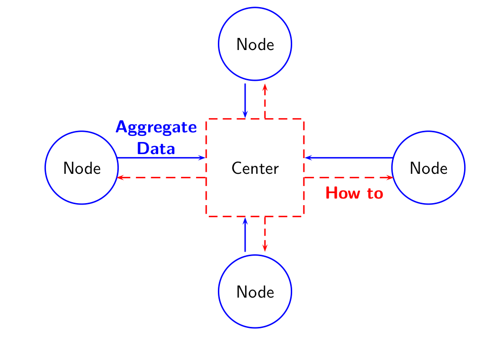
record. We assume that the center can direct the nodes as to how to
aggregate the covariates and can receive aggregate data from nodes
(Figure 1).
The implementation begins with the analytical center identifying the number of case and control subjects in the study cohort. Each node can send the number of cases and controls to the center without compromising privacy. The next step is to determine the pool size and creating random partition separately among cases and controls to identify which patients will contribute to which pool. To achieve this with, say, cases and controls, we randomly partition the cases and controls in and groups respectively. Suppose, subjects belongs to the case pool (), and subjects belongs to the case pool (). These pool memberships are passed onto the networks nodes to create pooled covariate values. After the pooled covariate values are returned to the analytical center, an analysis dataset is created based on the pooled covariate values and logistic regression is run on the pooled values to estimate covariate-specific ORs.
The process can be described step by step as follows:
- 1.
After applying appropriate inclusion and exclusion criteria, determine the number of cases () and controls () in the study cohort.
- 2.
Determine the pool size (if and have common divisor) or multiple pool sizes.
- 3.
Assuming , randomly partition cases in groups with case ids belonging to the case pool.
- 4.
Assuming , randomly partition controls in groups with control ids belonging to the control pool.
- 5.
Pass a case-id dataset to the nodes of the networks (see Table 1) to aggregate covariate for the cases.
- 6.
Pass a control-id dataset to the nodes of data networks similar to the case-id dataset to aggregate covariates for the controls. The case-id dataset and the control-id dataset will be the basis for pooling covariate values.
Table 1: Case-id dataset will consists of the pool id and the case ids contributing to specific pool. Pool id case id 1 case id 2 case id ⋮ ⋮ ⋮ ⋮ ⋮ ⋮ ⋮ ⋮ - 7.
Nodes work among themselves to pool the appropriate covariate values according to the case-id and control-id datasets and pass that to the analytic center.
- 8.
Analytical center uses a dataset as in Table 2 and runs logistic regression using case pool status (yes/no) as outcome and pooled covariate values.
| Case Pool | Pool id | Pooled Covariate value |
|---|---|---|
| Yes | ||
| ⋮ | ⋮ | |
| Yes | ||
| No | ||
| ⋮ | ⋮ | |
| No |
In addition to a primary exposure, confounders can be accommodated in a similar fashion as outlined before. In an epidemiological context, only categorical effect modifiers can be accommodated in PoLoR. Moreover, transformation of the covariate cannot be handled in PoLoR. In contrast, in the context of patient privacy, these issues can be addressed because individual level data is already collected and is available at the node level. It is easy to see that by using random pooling conditional only on the outcome, we can essentially circumvent these issues to (1) estimate all the components of the effect modifiers including the main effect and interaction and (2) accommodate continuous effect modifiers. Transformations can be handled in a similar manner: instead of sending , pooled level of appropriate transformation, such as can be made available to the center. Care should be taken in the choice of when multiple functional forms of the same covariates are included in the model. For example, if a cubic power and all lower powers of exposure is included in the model, then use of would divulge the individual patient covariate values. However, even in this case, it will not be possible to extract exact covariate combination for an individual participant.
As mentioned earlier, multiple pool sizes can be accommodated with the only stipulation that at least one pool of a specific size should be present in both case and control pools. However, unlike the standard approach, due to privacy concerns, we would not be able to create pools of size 1 in distributed data setting. We recommend choosing pool sizes to exhaust both and ; otherwise, excluding a very small number of observations from cases and controls. Not including these small number of samples in the analysis will likely minimally impact estimation and efficiency and will still keep patient records private. For example, if there are cases and controls, one can use pool sizes of and , with pools of size and pools of size among cases and pools of size and pools of size among controls. Otherwise, one can use pool of size only and exclude one control observation altogether from consideration.
In a distributed data setting, much of the limitation of the traditional setting, in particular for model selection, can be circumvented simply because individual level data can be accessed at the node level. For example, choosing between alternate transformations of the primary covariate of interest or confounder and EM would only require that center resend the new functional form to the nodes and nodes send back the pooled values according the transformation, while keeping the pool memberships the same as before. Hence, all standard diagnostics for logistic regression model can be adapted here. However, appropriateness of logit link still cannot be assessed in this setting using the existing tools.
Additional Considerations for Privacy
Secure summation: In addition to pooling of the covariate
value, secure summation can be employed to further protect individual
records. A simple secure
summation protocol would require generation of random numbers for each
pool and/or each node (and/or each covariate). After pooling the
covariate level for a given pool, the node adds a random number to the
pooled covariate value and passes this on to the next node. The next
node, adding the covariate values from appropriate pools, again add a
random number and pass on to other node as appropriate. When the
aggregate levels of the covariates reach the center, the nodes also
pass along the set of random number that were added to the
pools. Finally, the center subtracts the random numbers as appropriate
and works with the aggregate covariate values. If multiple nodes are
not colluding, secure summation is a very secure process. For more
details about secure summation, see, Karr et al., (2007).
Randomizing the order of the nodes for summation: For a
given pool, when multiple covariates need to be aggregated, we can
randomly order the nodes to add another layer of security. For
example, if nodes 1, 2, and 3 contribute to pool 1 for two variables,
then for one of the variables, the secure summation may begin with
node 1, then node 3 and finally end with node 2, while for the second
variable, the secure summation can follow the order: 3, 1, 2. Of
course, only the center should have the information about the
randomization scheme while nodes could have a limited information so
that they can pass the aggregate value to the appropriate nodes.
3 Example
3.1 Simulated Data
To demonstrate the viability of pooled analysis in a setting where individual-level covariate information can be accessed but not shared, we carried out simulation studies. Our earlier research and that of our collaborators established that pooled analysis produces consistent estimator of an exposure subject to pooling, a confounder (may or may not be subject to pooling) and interaction parameter for a categorical EM (Weinberg and Umbach,, 1999, Saha-Chaudhuri and Weinberg,, 2013, Saha-Chaudhuri et al.,, 2011). For a binary outcome, we demonstrate the feasibility of pooling in a distributed data context with transformation of a confounder and show that all parameters associated with a continuous EM can be consistently estimated using pooled analysis.
We considered simulated datasets each with a sample size of . The primary exposure was assumed to be normally distributed. The confounder was distributed as an absolute value of standard normal variable that had a correlation of with the primary exposure. Finally, a continuous EM was generated as standard normal independent of both and . The following model was considered for the binary outcome generation:
We considered several combination of parameter values and show the results for the following set: , resulting in a prevalence of . We used all observations for standard analysis.
For pooled analysis, we considered pools of sizes: conditional on the outcome status. To simplify the setting, we discarded at most observations from cases and/or controls when the and/or were not divisible by . Simulation for the entire setup was performed in the programming language R. In Table 3 we report the average parameter estimate, average model-based standard error (SE) and coverage probability out of simulations. In Figure 2, we plotted the parameter estimates from the standard analysis and pooled analysis (with ) to assess the agreement between the two sets of parameter estimates.
| Pooled | |||||
|---|---|---|---|---|---|
| Unpooled | g=2 | g=3 | g=4 | g=6 | |
| Estimate | 0.2499 | 0.2500 | 0.2500 | 0.2504 | 0.2502 |
| ModelSE | 0.0245 | 0.0253 | 0.0262 | 0.0272 | 0.0293 |
| Coverage | 0.9540 | 0.9400 | 0.9560 | 0.9400 | 0.9480 |
| Estimate | -0.3004 | -0.3007 | -0.3009 | -0.3013 | -0.3022 |
| ModelSE | 0.0175 | 0.0184 | 0.0193 | 0.0203 | 0.0224 |
| Coverage | 0.9580 | 0.9580 | 0.9520 | 0.9540 | 0.9520 |
| Estimate | 0.1507 | 0.1508 | 0.1513 | 0.1504 | 0.1514 |
| ModelSE | 0.0243 | 0.0251 | 0.0259 | 0.0268 | 0.0288 |
| Coverage | 0.9620 | 0.9540 | 0.9500 | 0.9520 | 0.9700 |
| Estimate | 0.5002 | 0.5006 | 0.5003 | 0.5016 | 0.5005 |
| ModelSE | 0.0225 | 0.0237 | 0.0250 | 0.0264 | 0.0294 |
| Coverage | 0.9320 | 0.9340 | 0.9360 | 0.9220 | 0.9440 |
Comparing the parameter estimates, model-based SE and coverage for the four parameters of the model between standard logistic regression and PoLoR, we see that on an average PoLoR performs comparably to standard analysis. Given that pooling essentially reduce the data dimension, we see a tendency of increased model-based SE, especially for larger poolsizes. However, the corresponding coverage of the model-based CI is generally close to the nominal coverage.
We also plotted the estimates of the four parameters () from each of the simulations obtained via standard logistic regression and PoLoR with in Figure 2 to demonstrate the comparability between two sets of estimates over each simulation. We added a diagonal line (black, dashed) and the lowess line (red, solid) to the plots. The red lowess line is generally in agreement with the diagonal black line indicating the similarity between the two sets of estimates.
Practical Consideration: Poolsize Recommendation
In the simulation settings we considered with a sample size of 30,000,
poolsizes between produced PoLoR estimates that were
comparable to the estimates from standard logistic regression. Due to
regression to the mean, larger poolsizes, especially, for a skewed
covariate, produced estimates that were biased away from
null. Therefore, we do not recommend poolsizes larger than
. Poolsizes (or smaller) performed well for different
exposure distributions. For distributed data setting, between
could be used to achieve a balance between privacy and unbiased
estimation.
3.2 Real Data
We demonstrate the comparability of PoLoR with standard logistic regression using a modified version of data from one of the first successful trials of adjuvant therapy regimens for colon cancer. The original study compared two treatment: Levamisole, and combination of Levamisole and Fluorouracil against observation only arm using a randomized controlled clinical trial among stage III colon cancer patients (Laurie et al.,, 1989). Due to strong evidence of benefit from the combination of Levamisole and Fluorouracil, the trial was stopped early. The dataset (data(colon)) has been downloaded from R library survival and is closest to that of the final report by Moertel et al., (1995).
In the original dataset, each patient contributed two time-to-event outcomes: time to recurrence and time to survival. We use only the time to recurrence and converted the endpoint to a binary outcome using “recurrence-free for 5 years” (yes/no) as an endpoint. Fifty five patients censored before 5 years and 22 patients with missing tumor differentiation status were excluded, leaving 866 patients. For standard logistic regression and PoLoR, we included the following variables in the model: sex (female:0, male:1), age (in years), obstruction of colon by tumor (yes/no), perforation of colon (yes/no), adherence of tumor to nearby organs (yes/no), tumor differentiation (1=well, 2=moderate, 3=poor), more than 4 positive nodes (yes/no), and treatment (observation only, Levamisole and Levamisole+Fluorouracil).
For PoLoR, we aggregated the variables using poolsizes and resulting in and pools respectively. Two patients were excluded at random to create the pools. Larger poolsizes were not considered due to relatively modest sample size of 866. The pools were created randomly. The parameter estimates of PoLoR are dependent on the particular pool formation and can differ according to different pool formation. We report the estimates based on one particular realization. For demonstration purpose, we considered age as a confidential variable. We created pool ids at random and aggregated all variables except age according to the pool ids. Instead of aggregating age, we aggregated a perturbed age variable by adding a random integer between 1 and 20 to the observed age. Aggregate age was then derived from the perturbed age by subtracting the aggregate of the random numbers. Finally we analysed the pooled data using PoLoR with the appropriate offset. We list the log OR and the SE for each of the covariate for standard logistic regression and PoLoR () in Table 4. In general, the direction and magnitude of the log ORs are similar between standard logistic regression and PoLoR, except for the variables perforation (only 27 patients with perforation) and differentiation (91 patients without differentiation). The SEs are generally comparable.
| Log Odds Ratio | |||
| Standard Error | |||
| Variable | Std logit | PoLoR | PoLoR |
| Sex | -0.149 | -0.044 | -0.158 |
| 0.144 | 0.163 | 0.180 | |
| Age | -0.003 | -0.006 | -0.012 |
| 0.006 | 0.007 | 0.008 | |
| Obstruction | 0.096 | 0.117 | 0.143 |
| 0.183 | 0.190 | 0.201 | |
| Perforation | 0.466 | 0.531 | 0.154 |
| 0.430 | 0.465 | 0.512 | |
| Adherence | 0.408 | 0.346 | 0.612 |
| 0.208 | 0.221 | 0.247 | |
| Differentiation=2 | -0.092 | 0.228 | 0.208 |
| 0.236 | 0.265 | 0.272 | |
| Differentiation=3 | 0.163 | 0.632 | 0.603 |
| 0.288 | 0.334 | 0.338 | |
| Node4 | 1.238 | 1.067 | 1.231 |
| 0.171 | 0.187 | 0.215 | |
| Levamisole | -0.145 | -0.285 | -0.182 |
| 0.174 | 0.209 | 0.225 | |
| Lev+FU | -0.750 | -0.788 | -0.880 |
| 0.178 | 0.210 | 0.236 | |
4 Discussion
In this manuscript, we introduce PoLoR (Pooled Logistic Regression) as a privacy-preserving approach to estimate coefficients of a logistic regression model using only aggregate covariate level. PoLoR is an existing idea from observational and epidemiologic study setting and can be adapted for distributed data network while maintaining patient privacy. PoLoR, being based on aggregate covariate level also reduces data dimension and hence can be used to analyze big data under a resource-constrained setting.
PoLoR is primarily intended for an exposure that is measured in an assay (e.g., blood, serum, urine, etc.) and pooling specimen from multiple study subjects leads to a reduced overall assay cost. We show here that covariate pooling approach or microaggregation for logistic regression can be applied in a non-assay setting to protect patient privacy. PoLoR is an application of specimen pooling for distributed data. In PoLoR, estimation of model parameters is based only on the aggregate covariate level rather than individual covariate level. Adopting this strategy in a distributed data setting would imply that only aggregate covariate information is needed to estimate ORs associated with covariates. Since aggregate covariate levels does not reveal individual information, it can be shared without compromising patient privacy and hence is suitable in a distributed data setting. For a binary outcome and a discrete time-to-event outcome, the model parameters between PoLoR and a standard logistic regression based on individual covariate levels remain the same, thus allowing estimation of the parameters of interest using aggregate covariate values.
However, PoLoR is not without limitations. PoLoR is scalable for larger number of nodes. But to ensure valid parameter estimates, it is important to keep track of the pools and which patients (from which node) are contributing to a given pool. For maintaining patient privacy in PoLoR, we need to create reasonably large pool size and therein lies the dilemma of choosing an appropriate poolsize . For PoLoR, the unit of measurement is pools and not individuals, so the asymptotic properties of the estimators will be somewhat dependent on the number of pools rather than the number of individuals. Thus, for asymptotic properties of the estimators, such as nominal confidence level, to hold, we need large number of pools, which in turn implies that we cannot use that is too large compared to and , because and will need to be large for asymptotic properties to hold. In our simulations, a poolsize between achieves a reasonable balance between unbiasedness and privacy and that is what we recommend. We do not recommend even for a very large dataset due to regression to mean and resulting bias in parameter estimates. If privacy is of no concern, another important issue would be to assess the properties of PoLoR when we use different for cases and control and in particular use a small value of for cases and a large value of for controls with only one pool of size among controls and one pool of size among cases. Also, PoLoR is meant for one time application only. Addition of a new patient record would require creating pools afresh and similar to standard logistic regression, would require reanalysis.
Several important issues warrant additional research. One can show that PoLoR can be used for a discrete survival outcome. Frequently though, survival outcome is continuous and currently there is no method for analyzing survival outcome in a distributed data setting. Another important extension could be for longitudinal outcome. Conceivably, PoLoR would likely be applicable in longitudinal setting, but the details need to be worked out. We surmise that other approaches in the infectious disease setting that uses pooling could be adapted for distributed data setting. This may open up several opportunities for analyzing distributed data. Finally, approaches from statistical disclosure limitation may be borrowed for distributed data while maintaining patient privacy.
Acknowledgement
References
- Caudill, (2010) Caudill, S. P. (2010). Characterizing populations of individuals using pooled samples. Journal of Exposure Science and Environmental Epidemiology, 20: 29–37.
- Cook et al., (2012) Cook, A., Wellman, R., Marsh, T., Tiwari, R., Nguyen, M., Russek-Cohen, E., Jiang, Z., and Nelson, J. (2012). Mini-sentinel methods development: Statistical methods for estimating causal risk differences in the distributed data setting for postmarket safety outcomes. Technical report, FDA’s Sentinel Initiative.
- Domingo-Ferrer and Mateo-Sanz, (2002) Domingo-Ferrer, J. M. and Mateo-Sanz, J. (2002). Practical data-oriented microaggregation for statistical disclosure control. IEEE Transactions on Knolwedge and Data Engeneering, 14: 189–201.
- Dorfman, (1943) Dorfman, R. (1943). The detection of defective members of large populations. Annals of Mathematical Statistics, 14: 436–440.
- Dwork, (2006) Dwork, C. (2006). Differential privacy. In Proceedings of the 33rd International Colloquium on Automata, Languages and Programming, volume 4052 of LNCS, pages 1–12. Springer-Verlag.
- El Emam et al., (2013) El Emam, K., Samet, S., Arbuckle, L., Tamblyn, R., Earle, C., and Kantarcioglu, M. (2013). A secure distributed logistic regression protocol for the detection of rare adverse drug events. Journal of the American Medical Informatics Association, 20(3): 453–461.
- Faraggi et al., (2003) Faraggi, D., Reiser, B., and Schisterman, E. F. (2003). ROC curve analysis for biomarkers based on pooled assessments. Statistics in Medicine, 22: 2515–2527.
- Fienberg et al., (2006) Fienberg, S. E., Fulp, W. J., Slavkovic, A. B., and Wrobel, T. A. (2006). "Secure" log-linear and logistic regression analysis of distributed databases. In Domingo-Ferrer, J. and Franconi, L., editors, Privacy in Statistical Databases, volume 4302 of Lecture Notes in Computer Science, pages 277–290. Springer Berlin Heidelberg.
- Fienberg et al., (2009) Fienberg, S. E., Nardi, Y., and Slavkovic, A. B. (2009). Valid statistical analysis for logistic regression with multiple sources. In Gal, C., Kantor, P., and Lesk, M., editors, Protecting Persons While Protecting the People, volume 5661 of Lecture Notes in Computer Science, pages 82–94. Springer Berlin Heidelberg.
- Filion et al., (2014) Filion, K. B., Chateau, D., Targownik, L. E., Gershon, A., Durand, M., Tamim, H., Teare, G. F., Ravani, P., Ernst, P., Dormuth, C. R., and the CNODES Investigators (2014). Proton pump inhibitors and the risk of hospitalisation for community-acquired pneumonia: replicated cohort studies with meta-analysis. Gut, 63(4): 552–558.
- Gunn et al., (2004) Gunn, P. P., Fremont, A. M., Bottrell, M., Shugarman, L. R., Galegher, J., and Bikson, T. (2004). The health insurance portability and accountability act privacy rule: a practical guide for researchers. Med Care, 42(4): 321–7.
- Huang and Pepe, (2010) Huang, Y. and Pepe, M. S. (2010). Assessing risk prediction models in case-control studies using semiparametric and nonparametric methods. Statistics in Medicine, 29(13): 1391–1410.
- Karr et al., (2007) Karr, A. F., Fulp, W. J., Vera, F., Young, S. S., Lin, X., and Reiter, J. P. (2007). Secure, privacy-preserving analysis of distributed databases. Technometrics, 49: 335–345.
- Laurie et al., (1989) Laurie, J. A., Moertel, C. G., Fleming, T. R., Wieand, H. S., Leigh, J. E., Rubin, J., McCormack, G. W., Gerstner, J. B., Krook, J. E., and Malliard, J. (1989). Surgical adjuvant therapy of large-bowel carcinoma: An evaluation of levamisole and the combination of levamisole and fluorouracil: The north central cancer treatment group and the mayo clinic. J Clinical Oncology, 7: 1447–1456.
- Liu and Schisterman, (2003) Liu, A. and Schisterman, E. F. (2003). Comparison of diagnostic accuracy of biomarkers with pooled assessments. Biometrical Journal, 45: 631–644.
- Moertel et al., (1995) Moertel, C. G., Fleming, T. R., Macdonald, J. S., Haller, D. G., Laurie, J. A., Tangen, C. M., Ungerleider, J. S., Emerson, W. A., Tormey, D. C., Glick, J. H., Veeder, M. H., and Mailliard, J. A. (1995). Fluorouracil plus levamisole as effective adjuvant therapy after resection of stage iii colon carcinoma: A final report. Annals of Internal Medicine, 122(5): 321–326.
- Nattinger et al., (2010) Nattinger, A. B., Pezzin, L. E., Sparapani, R. A., Neuner, J. M., King, T. K., and Laud, P. W. (2010). Heightened attention to medical privacy: Challenges for unbiased sample recruitment and a possible solution. American Journal of Epidemiology, 172(6): 637–644.
- Ness, (2010) Ness, R. B. (2010). Invited commentary: Population-based human subjects research in the era of enhanced privacy regulation. American Journal of Epidemiology, 172(6): 648–650.
- Olsen, (2014) Olsen (2014). Data protection and epidemiological research: a new EU regulation is in the pipeline. International Journal of Epidemiology, 43(5): 1353–1354.
- Saha-Chaudhuri et al., (2011) Saha-Chaudhuri, P., Umbach, D. M., and Weinberg, C. R. (2011). Pooled exposure assessment for matched case-control studies. Epidemiology, 22(5): 704–712.
- Saha-Chaudhuri and Weinberg, (2013) Saha-Chaudhuri, P. and Weinberg, C. R. (2013). Specimen pooling for efficient use of bio-specimens in studies of time to a common event. American Journal of Epidemiology, 178: 126–135.
- Sham et al., (2002) Sham, P., Bader, J. S., Craig, I., O’Donovan, M., and Owen, M. (2002). Dna pooling: a tool for large-scale association studies. Nature Reviews Genetics, 3: 862–871.
- Stein et al., (2009) Stein, C. R., Savitz, D. A., and Dougan, M. (2009). Serum levels of perfluorooctanoic acid and perfluorooctane sulfonate and pregnancy outcome. American Journal of Epidemiology, 170(7):837–846.
- Suissa et al., (2012) Suissa, S., Henry, D., Caetano, P., Dormuth, C. R., Ernst, P., Hemmelgarn, B., Lelorier, J., Levy, A., Martens, P. J., Paterson, J. M., Platt, R. W., Sketris, I., and Teare, G. (2012). CNODES: the Canadian Network for Observational Drug Effect Studies. Open Med, 6(4): e134–40.
- Wang et al., (2013) Wang, S., Jiang, X., Wu, Y., Cui, L., Cheng, S., and Ohno-Machado, L. (2013). EXpectation Propagation LOgistic REgression (EXPLORER): Distributed privacy-preserving online model learning. Journal of Biomedical Informatics, 46(3): 480–496.
- Weinberg and Umbach, (1999) Weinberg, C. R. and Umbach, D. M. (1999). Using pooled exposure assessment to improve efficiency in case-control studies. Biometrics, 55: 718–726.
- Wolfson et al., (2010) Wolfson, M., Wallace, S. E., Masca, N., Rowe, G., Sheehan, N. A., Ferretti, V., LaFlamme, P., Tobin, M. D., Macleod, J., Little, J., Fortier, I., Knoppers, B. M., and Burton, P. R. (2010). DataSHIELD: resolving a conflict in contemporary bioscience-performing a pooled analysis of individual-level data without sharing the data. International Journal of Epidemiology, 39: 1372–1382.
- Wu et al., (2012) Wu, Y., Jiang, X., Kim, J., and Ohno-Machado, L. (2012). Grid binary logistic regression (glore): building shared models without sharing data. Journal of the American Medical Informatics Association, 19(5):758–764.
- Yu et al., (2015) Yu, O. H. Y., Filion, K. B., Azoulay, L., Patenaude, V., Majdan, A., and Suissa, S. (2015). Incretin-based drugs and the risk of congestive heart failure. Diabetes Care, 38(2): 277–284.