Exact Clustering of Weighted Graphs via Semidefinite Programming
Abstract
As a model problem for clustering, we consider the densest -disjoint-clique problem of partitioning a weighted complete graph into disjoint subgraphs such that the sum of the densities of these subgraphs is maximized. We establish that such subgraphs can be recovered from the solution of a particular semidefinite relaxation with high probability if the input graph is sampled from a distribution of clusterable graphs. Specifically, the semidefinite relaxation is exact if the graph consists of large disjoint subgraphs, corresponding to clusters, with weight concentrated within these subgraphs, plus a moderate number of nodes not belonging to any cluster. Further, we establish that if noise is weakly obscuring these clusters, i.e, the between-cluster edges are assigned very small weights, then we can recover significantly smaller clusters. For example, we show that in approximately sparse graphs, where the between-cluster weights tend to zero as the size of the graph tends to infinity, we can recover clusters of size polylogarithmic in under certain conditions on the distribution of edge weights. Empirical evidence from numerical simulations is also provided to support these theoretical phase transitions to perfect recovery of the cluster structure.
1 Introduction
Clustering is a fundamental problem in machine learning and statistics, focusing on the identification and classification of groups, called clusters, of similar items in a given data set. Clustering is ubiquitous, playing a prominent role in varied fields such as computational biology, information retrieval, pattern recognition, image processing and computer vision, and network analysis. This problem is inherently ill-posed, as the partition or clustering of any given data set will depend heavily on how we quantify similarity between items in the data set and how we characterize clusters; it is not outside the realm of possibility to have two drastically different clusterings of the same data if two different similarity metrics are used in the clustering process. Regardless of the similarity metric used, clustering is a combinatorial optimization problem at its core: given data, identify a partition or labeling of the data (approximately) maximizing some measure of quality of the clustering. Due to the difficulties inherent with optimization over discrete sets, many popular approaches for clustering involve the approximate solution of an NP-hard combinatorial optimization problem; for example, the spectral clustering heuristic for the normalized cut problem (Dhillon et al., 2004; Ng et al., 2002), the convex relaxation approaches for the correlation clustering problem (Mathieu and Schudy, 2010), robust principal component analysis (Chen et al., 2014a; Oymak and Hassibi, 2011), and the densest -disjoint-clique problem (Ames and Vavasis, 2014; Ames, 2014), among many others.
In spite of the inherent intractability of clustering, many recent analyses have established that if data is sampled from some distribution of clusterable data, then one can efficiently recover the underlying cluster structure using a variety of clustering algorithms. In particular, the recent results of Abbe et al. (2016); Ailon et al. (2013); Ames and Vavasis (2014); Ames (2014); Amini and Levina (2018); Cai and Li (2015); Chen et al. (2014a); Chen et al. (2014b); Chen and Xu (2014); Guédon and Vershynin (2015); Hajek et al. (2015); Lei and Rinaldo (2015); Mathieu and Schudy (2010); Nellore and Ward (2015); Oymak and Hassibi (2011); Rohe et al. (2011); Qin and Rohe (2013); Vinayak et al. (2014) all establish sufficient conditions under which we can expect to identify the latent cluster structure efficiently. Most of these results assume that the similarity structure of the data can be modeled as a graph sampled from some generalization of the stochastic block model proposed by Holland et al. (1983). In this model, the nodes of the graph, called the similarity graph of the data, are associated with the items in the data set. An edge is drawn between two items with fixed probability if the corresponding items belong to the same cluster, and with fixed probability if the corresponding items belong to different clusters. Under this block model, the analyses cited above establish that the block structure of the data can be recovered in polynomial-time with high probability provided that the smallest cluster in the data is sufficiently large, typically larger than , where denotes the number of items in the data (and nodes in the similarity graph) and is a polylogarithmic factor in depending on .
Although valuable in establishing sufficient conditions for data to be clusterable, these results are not immediately applicable to data sets seen in many applications, particularly those arising from the analysis of social networks. For example, statistical analysis of social networks suggests that communities, playing the role of clusters, tend to be limited in size to several hundred users, while the networks themselves can contain thousands, if not millions or even billions, of users (Leskovec et al., 2008; Leskovec et al., 2009). However, the recent analyses of Chen et al. (2014a); Chen and Xu (2014); Guédon and Vershynin (2015); Jalali et al. (2015); Rohe et al. (2014), among others, suggest that these clusterability results are overly conservative with respect to the size of clusters we can expect to recover in polynomial-time. Specifically, these analyses allow the edge probabilities and to vary with , and investigate how the size of the smallest cluster that can be recovered depends on the relative scaling of and . In this case, the data is often assumed to be sampled from a sparse generalized stochastic block model where the parameters and governing edge formation are functions depending on the number of items and one or both tends to as . In the case where tends to much more slowly than , the noise obscuring the block structure is significantly weaker than in the dense graph case (where and are assumed fixed). Here, sparsity refers to the fact that graphs generated according to the block model contain very few edges between clusters with high probability when is large, and not that the graph itself is sparse in the sense that the nodes have small average degree. In this case, it has been shown that clusters significantly smaller than can be recovered efficiently; specifically, several methods have been shown to recover clusters with size polylogarithmic in under certain assumptions on the probability functions and (Chen et al., 2014a; Chen and Xu, 2014; Guédon and Vershynin, 2015; Rohe et al., 2014, see). We should note that these results provide evidence of a computational limit for cluster recovery; that is, these results establish that clusters can be recovered in a computationally efficient way if the underlying data satisfies certain sufficient conditions. We should note further that the lower bounds on cluster size given by these sufficient conditions typically do not match information-theoretic limits; it is well-known that it is possible to identify clusters of size on the order of in certain settings, however, no polynomial-time algorithms are known to do so (Chen and Xu 2014; Hajek et al. 2015 provide further details).
The primary contribution of this paper is an analysis establishing similar clusterability results for a particular convex relaxation of the clustering problem. That is, we present an analysis establishing the following theorem, which provides conditions for perfect recovery of the underlying cluster structure from the solution of a particular semidefinite program. As an immediate corollary, the theorem establishes that one may identify clusters as small as , i.e., there exists constant such that the size of the smallest cluster recoverable cluster is bounded below by for sufficiently large , with high probability if the data is sampled from the sparse block model described above for particular choices of and . Here, we say that an event occurs with high probability (w.h.p.) if the event occurs with probability tending polynomially to as .
Theorem 1.1.
Suppose that the -node graph is sampled from the generalized stochastic block model, with disjoint blocks, in-cluster edge probability , and between-cluster edge probability . Let denote the adjacency matrix of and let and denote the cardinality of the smallest and largest clusters, respectively, in the block model for . Then there exists constants such that the columns of the optimal solution of the semidefinite program
are scalar multiples of the characteristic vectors of the clusters in our underlying block model with high probability if
where , and
Moreover, in this case, every characteristic vector of a cluster in the block model is a scalar multiple of at least one column of .
Here, the characteristic vector of a set is the vector with th element
In Theorem 1.1, denotes the trace of the matrix , denotes the all-ones vector of appropriate dimension, the notation indicates that the entries of are nonnegative, and denotes the cone of symmetric positive semidefinite matrices.
Note that if is sampled from the dense block model, i.e., are independent of , then Theorem 1.1 suggests that we have exact recovery if with high probability, where is a constant depending on ; this bound matches that established by Ames (2014) (among many others) up to constant terms. On the other hand, when is sampled from the sparse block model, we see that Theorem 1.1 suggests that we may have perfect recovery of significantly smaller clusters. For example, suppose that is fixed and . Then we have exact recovery with high probability if the smallest cluster has size ; see the discussion following Theorem 2.2.
We will show that analogous phenomena occur in what we will call approximately sparse graphs. In many practical applications, the expectation that we have a binary labeling indicating whether any pair of items in a given data set are similar or dissimilar is unrealistic. However, it is often possible to describe the level of similarity between any two items using some affinity function based on distance between the items in question. For example, we could consider the discrepancy in pixel intensity and geographic location in image segmentation applications or Euclidean distance between two items represented as vectors in a Euclidean space (or some other vector space with corresponding norm). In this case, we can summarize the pairwise similarity relationships within our data using a weighted graph, called a weighted similarity graph. Specifically, given a data set with affinity function , the weighted similarity graph is the weighted complete graph with nodes corresponding to the items in the data set, and edge weight between nodes and given by the value of . Clearly, this contains the similarity graphs discussed earlier as a special case where if items and are known to be similar and otherwise; note that we assume that we have an undirected graph with symmetric adjacency matrix.
We can generalize the stochastic block model in an identical fashion. We assume that items in the same cluster are significantly more similar than pairs of items in different clusters. This corresponds to edge weights within clusters being larger, on average, than edge weights between clusters. This motivates the following random graph model, which we will call the planted cluster model. Let be the weighted complete graph whose node set represents the items in some data set containing clusters and (potentially) some nodes that will not be assigned to a cluster. For each pair of nodes in the same cluster , we randomly sample edge weight , and by symmetry, from some probability distribution with mean . If , , where , i.e., do not belong to the same cluster, we sample from a different probability distribution with mean . Note that this model contains the generalized stochastic block model discussed earlier as a special case when and are Bernoulli distributions with probabilities of success and , respectively.
It was shown by Ames (2014) that if is sampled from the planted cluster model with minimum cluster size at least in the homogeneous case where all within-cluster edges are i.i.d. with mean and all between-cluster edges are i.i.d. with mean , where is a constant depending on and , then we can recover the clusters from the optimal solution of the semidefinite program
| (1) |
with high probability, where is the number of clusters in the graph. We will show that these results can be strengthened to establish that much smaller clusters can be recovered in the presence of approximately sparse noise. That is, we will see that if the between-cluster edge weights have expectation and variance approaching zero sufficiently quickly as , then we may recover clusters containing as few as nodes with high probability. We will derive the semidefinite program (1) as a relaxation of a particular model problem for clustering in Section 2.1 and formally state our recovery guarantees in Section 2.2; we will see that these results immediately specialize to those stated in Theorem 1.1 for the semidefinite program (1.1).
2 Semidefinite Relaxations of the Densest k-Disjoint Clique Problem
In this section, we derive a semidefinite relaxation for the densest -disjoint clique problem and present an analysis illustrating a sufficient condition ensuring that this relaxation is exact. This problem will act as a model problem for clustering and we will see that we should expect to accurately recover the underlying cluster structure if the given data satisfies this sufficient condition.
2.1 The Densest k-disjoint Clique Problem
We begin by deriving a heuristic for the clustering problem based on semidefinite relaxation of the densest disjoint clique problem. A similar discussion motivating the relaxation was originally presented by Ames (2014); we repeat it here for completeness. Let be a weighted complete graph with vertex set and nonnegative edge weights for all . Given a subgraph of , the density of is the average edge weight incident at a vertex in :
If we assume that is the similarity graph of some data set consisting of disjoint clusters and that weight is concentrated more heavily on within-cluster edges than between-cluster edges, then we may cluster this data set by finding the set of disjoint subgraphs, corresponding to these clusters, with maximum density; we call this problem the densest -partition problem. Peng and Wei (2007) established that the densest -partition problem is NP-hard. Moreover, this partition model excludes the case where some items in the data set do not naturally associate with any of the clusters in the data. To simultaneously motivate a convex relaxation of the densest -partition problem and address the inclusion of nodes that do not naturally belong to clusters, we consider the densest -disjoint clique problem.
Given a graph , a clique of is a pairwise adjacent subset of . That is, is a clique of if for every pair of nodes or, equivalently, the subgraph induced by is complete. We say that is a -disjoint-clique subgraph of if consists of disjoint cliques, i.e., is the union of disjoint complete subgraphs of . The densest -disjoint-clique problem seeks a -disjoint-clique subgraph maximizing the sum of the densities of the disjoint complete subgraphs comprising . Note that if we add the additional constraint that each node in belongs to exactly one -disjoint-clique subgraph in , then the densest -disjoint-clique problem becomes the densest -partition problem. However, in general, the densest -disjoint-clique problem allows an assignment of nodes to clusters, represented by the disjoint cliques, which excludes some nodes. For example, if such nodes are present in the data, they would not be assigned to a cluster by the optimal -disjoint-clique subgraph.
The complexity of the densest -disjoint-clique problem is unknown; in particular, no polynomial-time algorithm for its solution is known. To address this potential intractability, we will attempt to approximately solve the -disjoint-clique problem by convex relaxation. Suppose that are the characteristic vectors of a set of disjoint cliques forming a -disjoint-clique subgraph of . Using this notation, the density of the complete subgraph induced by is equal to
If we let be the matrix with th column equal to , where denotes the standard Euclidean norm, then it is easy to see that
We call such a matrix a normalized -cluster matrix and denote the set of normalized -cluster matrices of the vertex set by . It follows that the densest -disjoint-clique problem may be formulated as
| (2) |
Again, the complexity of (2) is unknown, however, the maximization of quadratic functions subject to combinatorial constraints is known to be NP-hard.
A process for relaxation of (2) using matrix lifting is described by Ames (2014); a similar relaxation technique was applied by Ames and Vavasis (2011); Ames and Vavasis (2014) and Ames (2015). In particular, each proposed cluster , with characteristic vector , corresponds to the rank-one symmetric matrix
It is easy to see that the density of is equal to
Moreover, each of the matrices has row and column sums equal to either 0 or 1, and trace equal to 1. Finally, for each proposed clustering , the corresponding rank-one matrices are orthogonal in the trace inner product, due to the orthogonality of the characteristic vectors of the corresponding disjoint clusters. Thus, the matrix
| (3) |
has rank equal to . This suggests that we may relax (2) as the rank-constrained semidefinite program
| (4) |
The relaxation (4) can be relaxed further to a semidefinite program by omitting the nonconvex rank constraint:
| (5) |
We should note that the semidefinite program (5) is remarkably similar to the semidefinite relaxation of the minimum sum of squared distance partition of Peng and Wei (2007) and the semidefinite relaxation of the maximum likelihood estimate of the stochastic block model considered by Amini and Levina (2018), among others, although our relaxation approach differs slightly from that used in these two papers.
2.2 Block Models and Recovery Guarantees
Given a set of clusterable data or, more accurately, a clusterable graph representation of data, Ames (2014) established that one can recover the underlying cluster structure from the optimal solution of the semidefinite program (5). Specifically, it is assumed that data with strong cluster structure should correspond to similarity graphs with heavy weight assigned to edges within clusters, relative to that between cluster edges. This corresponds to pairs of items within clusters being significantly more similar than pairs of items in different clusters. This motivates the following block model.
Let be a -disjoint-clique subgraph of with vertex set composed of the disjoint cliques and let denote the set of all symmetric matrices. We consider weight matrices with entries sampled independently from one of two probability distributions as follows.
- •
For each and each , we sample from a distribution such that
for fixed .
- •
For each remaining edge , , we sample the edge weight from a second distribution such that
for fixed if or , and otherwise.
We should note that the assumption that the entries of are bounded between and is made for simplicity in the statement and proof of our main result; analogous recovery guarantees hold if we assume that random variables sampled according to and are bounded and nonnegative with high probability. We say that such random matrices are sampled from the planted cluster model. Note that if is sampled from the planted cluster model, then weight is concentrated on within-cluster edges (in expectation). This provides a natural generalization of the stochastic block model. Indeed, the stochastic block model corresponds to the planted cluster model in the special case that and are Bernoulli distributions with probabilities of success and , respectively. Ames (2014) established the following theorem, ensuring recovery of the planted cliques from the optimal solution of (5) under the planted cluster model (see Ames, 2014, Theorem 2.1).
Theorem 2.1.
Suppose that the vertex sets define a -disjoint-clique subgraph of the -node weighted complete graph and let . Let for all and let Let be a random symmetric matrix sampled from the planted cluster model according to distributions and with means and , respectively, satisfying
Let be the feasible solution of (5) corresponding to defined by (3). Then there exist scalars such that if
then is the unique optimal solution of (5), and is the unique maximum density -disjoint-clique subgraph of with probability tending exponentially to as .
In contrast to Theorem 1.1, the result of Theorem 2.1 implies that we can have perfect recovery if the graph contains a small number of nodes that shouldn’t be assigned to any of the planted clusters. Each potential edge from each of these nodes to any other node is added independently to the graph with probability , so that each node in has roughly the same number of neighbours in each cluster block. This implies that such a node is not assigned to any of the planted clusters because it is weakly associated with all of the planted clusters. It is important to note that this edge assignment is performed randomly and not deterministically by an adversary attempting to obscure the cluster structure present in the graph. We present a new analysis that improves upon the recovery guarantee of Theorem 2.1 in two ways. First, the hypothesis of Theorem 2.1 assumes that between-cluster and within-cluster edge weights are i.i.d. We consider the more general heterogeneous case constructed as follows:
- •
For each , , we sample the edge weight from distribution with
This forces weights within the same block to be i.i.d., but weight may not be identically distributed in different blocks.
Second, the analysis leading to Theorem 2.1 assumes that the expectations of in the planted cluster model are fixed and that the variances are bounded by . We improve upon the recovery guarantee of Theorem 2.1 by considering the case where the parameters and depend on the number of nodes in the graph. In particular, our recovery guarantees explicitly depend on the variances of the distributions , and their scaling with , which will expand the set of graphs known to be clusterable by (5). We have the following theorem.
Theorem 2.2.
Suppose that the vertex sets define a -disjoint-clique subgraph of the weighted complete graph on vertices and let . Let for all and let . Let be a random symmetric matrix sampled from the heterogeneous planted cluster model according to distributions with expected values and variances . Let and . Let be the feasible solution to (5) corresponding to defined by (3). Let
Then there exists scalar such that if
| (6) |
then is the unique optimal solution for (5), and is the unique maximum density -disjoint-clique subgraph of with high probability.
The weak assortativity condition (6) implies that we have perfect recovery provided that the gap between the cluster block expectation and the largest between-cluster block expectation is sufficiently large for all clusters , , relative to the minimum cluster size, number of unassigned nodes , number of clusters, and edge weight variances. In the Bernoulli case, i.e., within-cluster and between-cluster edges are added independently with probabilities and , respectively, Theorem 2.2 and, in particular, (6) establish that we can recover the planted clusters provided that
This result agrees with the Easy Regime for cluster recovery proposed by Chen and Xu (2014), where a polynomial-time algorithm exists for exact recovery of the planted clusters, in this case, the solution of the semidefinite relaxation (5). One distinct advantage of this result over similar recovery guarantees is that our model and phase transition are largely parameter free. For example, Amini and Levina (2018) present an analysis of three semidefinite relaxations that obtain nearly identical conditions on guaranteeing recovery but restrict their analysis to the case where the clusters are identical in size or otherwise known and when are Bernoulli distributions; we should note that Amini and Levina (2018) consider heterogeneous Bernoulli distributions where the within-cluster and between-cluster probabilities of adding an edge vary across clusters. Similarly, Chen and Xu (2014) and Jalali et al. (2015) give identical conditions for recovery (up to constants and logarithmic terms) in the Bernoulli case to those in Theorem 2.2 for semidefinite relaxations that require the sizes of the clusters to be used as input parameters (or all clusters to have identical size), neither of which are realistic assumptions in practice. In contrast, our approach achieves this recovery guarantee using only the desired number of clusters as a parameter. Further, our guarantee extends to the general weighted case where the vast majority of existing recovery guarantees for stochastic block models are restricted to the Bernoulli case.
It is important to note that tighter recovery guarantees than those provided by Theorem 2.2 are known for specific problem settings. This is a natural consequence of the more general framework of our analysis. For example, Yan et al. (2017) studies a convex relaxation for cluster recovery in the Bernoulli (unweighted) case. The main theorem of this article establishes conditions for perfect recovery that allow larger clusters to have higher variance, although specialized for the unweighted case. Moreover, Yan et al. (2017) consider the use of a tuning parameter to allow recovery without knowledge of the number of clusters . On the other hand, the results of Amini and Levina (2018); Jalali et al. (2015) also provide tighter recovery guarantees but require knowledge of cluster sizes. The key contribution of this work is the presentation of a recovery guarantee that extends to the weighted case without strict assumptions regarding input parameters, as well as the first-order method for solution of (1) discussed in detail in Section 4.
To further illustrate the consequences of Theorem 2.2, we consider several examples. In each, we assume that the graph is generated in the homogeneous setting where within-cluster weights are i.i.d. according to with mean and variance , and between-cluster weights are i.i.d. according to with mean and variance .
2.2.1 The Dense Case
When are fixed, we obtain the same recovery guarantee as before, up to constants and logarithmic terms: we have exact recovery w.h.p. if and for some constants and depending on and . Indeed, each of the pointwise maximums in the first three terms of (6) is bounded above by since , and if .
2.2.2 The Sparse Case
On the other hand, if noise in the form of between-cluster edge-weight is small, then we should expect to be able recover much smaller clusters. For example, suppose that is the Bernoulli distribution with probability of adding an edge and that is the Bernoulli distribution with probability of adding an edge (the assumption that is for the sake of simplicity in this example and we can expect analogous recovery guarantees for any tending slowly enough to ). Assume further that Finally, again for simplicity, assume that we have equally sized clusters of size and (). In this case, (6) holds if
since and the terms involving and are equal to zero. This implies that we have exact recovery of the planted clusters w.h.p. provided . This exceeds the state of the art recovery bound of established in Jalali et al. (2015) by a factor of . However, the convex relaxation proposed by Jalali et al. (2015) requires knowledge of , which is often an unrealistic expectation in practice; in contrast, our approach only requires knowledge of the number of clusters present in the data. Further, the requirement is enforced by the gap inequality (6), which itself is a consequence of the use of the Bernstein inequality to establish certain dual variables are nonnegative in the proof of Theorem 2.2 (see Section 3.1 for more details). It may be possible to improve this bound to with improved concentration inequalities but it is unclear what form these improvements may take.
2.2.3 The Planted Clique and Sparsest Subgraph
In the special case when and and are Bernoulli distributions, the planted cluster model specializes to the planted clique model considered in Ames and Vavasis (2011) and Ames (2015). In this case, (6) suggests that we can recover a planted clique (in the dense case) of size . This recovery guarantee is far more conservative than those provided by Ames and Vavasis (2011) and Ames (2015), among others, which establish that a planted clique of size can be recovered from the optimal solution of a particular nuclear norm relaxation of the maximum clique problem.
Unfortunately, it appears that this lower bound restricting the size of a recoverable planted clique to a constant multiple of the number of nonclique vertices is tight. For example, let and be the probabilities of adding an edge given by and . Then the expected value of the proposed solution in (5) is equal to
On the other hand, the solution is also feasible for (5) with expected objective value
for some constant . This implies that the proposed solution is suboptimal if , which holds unless . We will see that the realized values of these sums are concentrated near their expectations and thus we cannot reasonably expect to recover planted clusters with unassigned nodes significantly outnumbering the smallest cluster. This implies that we cannot recover planted cliques of size by maximizing density of a complete subgraph because the planted clique is not the index set of the densest such graph; in this case, the entire graph is a denser complete subgraph, as measured by average vertex degree, in expectation.
3 Derivation of the Recovery Guarantee
In this section, we show that if the hypothesis of Theorem 2.2 is satisfied then the solution constructed according to (3) is optimal for (5) and the corresponding -disjoint-clique subgraph has maximum density. In particular, we will show that satisfies the following sufficient condition for optimality of a feasible solution of (5) (see Ames, 2014, Theorem 4.1).
Theorem 3.1.
Theorem 3.1 is a restriction of the Karush-Kuhn-Tucker optimality conditions to the semidefinite program (5) (see, for example, Boyd and Vandenberghe, 2004, Section 5.5.3). The goal of this section is to establish that we can construct dual variables , , and which satisfy the hypothesis of Theorem 3.1 with high probability if the weight matrix is sampled from a distribution of clusterable block models. To motivate our proposed choice of dual variables, we note that the complementary slackness condition holds if and only if under the assumption that both and are positive semidefinite. Therefore, the block structure of implies that each block of corresponding to a cluster block in must sum to zero.
Before we continue with the construction of our dual variables, let us first remind ourselves of the notation of Theorem 2.2. Let be a -disjoint-clique subgraph of with vertex set composed of the disjoint cliques of sizes and let be the corresponding feasible solution of (5) defined by (3). Let and be the size of . Moreover, let and be the size of the smallest and largest clusters, respectively. Let be a random symmetric matrix sampled from the planted cluster model with planted clusters and remaining nodes according to the distributions with means and variances .
We now propose a choice of dual variables satisfying the complementary slackness condition . Restricting this condition to the blocks and of and with rows and columns indexed by , , we see that holds if and only if
by the block structure of ; note that is chosen to satisfy the complementary slackness condition (9). Solving this linear system for using the Sherman-Morrison-Woodbury Formula (Golub and Van Loan, 2013, Equation (2.1.4)) gives
| (11) |
On the other hand, we choose to satisfy the complementary slackness condition (8). Next, we use this choice of to construct the remaining dual variables.
Fix such that . We will choose so that and . In particular, we choose
|
|
(12) |
where the vectors and are unknown vectors parametrizing the entries of ; here is the Kronecker delta function defined by if and otherwise. That is, we choose to be the expected value of plus the parametrizing term ; the vectors and are chosen to be solutions of the systems of linear equations given by the complementary slackness conditions and . It is reasonably straight-forward to show that we may choose
| (13) |
where
| (14) |
Indeed, we must choose and to be solutions of the system
| (15) |
to ensure that the complementary slackness conditions are satisfied. Note that taking the inner product of each side of (15) with the vector yields
by the symmetry of . This establishes that the solution of (15) is also a solution of the (singular) system of equations,
imposed by the complementary slackness conditions and . Solving (15) for and using the Sherman-Morrison-Woodbury Formula yields the formula for and given by (13). We set the remaining block . Ames (2014, Section 4.2) provides further details.
Finally, we choose
| (16) |
where is a parameter to be chosen later. In particular, the analysis provided in Sections 3.1, 3.2, and 3.3 establishes that a suitable choice of exists if the hypothesis of Theorem 2.2 is satisfied.
The entries of are chosen according to the stationarity condition (7), but we will also define an auxiliary variable as the following block matrix:
| (17) |
We next provide the following theorem, first stated by Ames (2014, Theorem 4.2), which characterizes when the proposed dual variables satisfy the hypothesis of Theorem 3.1.
Theorem 3.2.
Suppose that the vertex sets define a -disjoint-clique subgraph of the weighted complete graph , where is a random symmetric matrix sampled from the planted cluster model according to the distributions with means and variances . Let , and be defined as in Theorem 2.2. Let be the feasible solution for (5) corresponding to defined by (3). Let and be chosen according to (16), (11), and (12), respectively, and let be chosen according to (17). Suppose that the entries of and are nonnegative. Then is optimal for (5), and is the maximum density -disjoint-clique subgraph of corresponding to , if
| (18) |
Moreover, if (18) is satisfied and
| (19) |
for all such that , then is the unique optimal solution of (5) and is the unique maximum density -disjoint-clique subgraph of .
The proof of Theorem 3.2 is nearly identical to that by Ames (2014, Theorem 4.2), and is omitted. Theorem 3.2 provides a clear roadmap for the remainder of the proof; if we can show that if is sampled from the planted cluster model satisfying (6) then and are nonnegative and with high probability, then we will have established that we can recover the underlying block structure with high probability in this case. We establish the necessary bounds on and in the following sections.
3.1 Nonnegativity of and
We first establish that the entries of , as constructed according to (12), are nonnegative with high probability. To do so, we will make repeated use of the following specialization of the Bernstein inequality which provides a bound on the tail of a sum of bounded independent random variables; see Boucheron et al. (2013, Section 2.8), for more details regarding the Bernstein inequality.
Theorem 3.3.
Let be independent identically distributed (i.i.d.) variables with mean and variance . Let . Then
| (20) |
for all .
The following bound on the parametrizing vectors and in the choice of the block of defined by (12) is an immediate consequence of Theorem 3.3.
Lemma 3.1.
There exists constant such that
w.h.p., where , for all such that .
For such that , we define and as in (13). To bound the absolute values of the entries of and , we must estimate the sums , and ; applying Theorem 3.3 to bound the tails of these sums yields Lemma 3.1. See Appendix A for the full argument.
We have the following bound on the entries of as an immediate consequence of Lemma 3.1.
Proposition 3.1.
Suppose that satisfy (6). Then there exists constant such that each entry of is nonnegative w.h.p. if satisfies
| (21) |
Proof.
Fix such that . By construction, we have
Using (16) and Lemma 3.1, we see that
for all , w.h.p., where is the constant appearing in Lemma 3.1. Note that the right-hand side of this inequality is nonnegative if and only if
The argument for the case when one of or is equal to follows analogously. Applying the union bound over all blocks of shows that each entry of is nonnegative w.h.p. if satisfies (21). ∎
We have an analogous result ensuring that the entries of are nonnegative with high probability; we present the proof of this result in Appendix B.
Proposition 3.2.
Suppose satisfy (6). Then there exists constant such that each entry of is nonnegative w.h.p. if satisfies
| (22) |
for all .
We conclude this section with a result ensuring that the uniqueness condition (19) of Theorem 3.2 is satisfied for all such that ; we provide a proof in Appendix C.
Proposition 3.3.
Suppose that
| (23) |
Then for all such that with high probability.
3.2 A Bound on
It remains to establish the following bound on the spectral norm of the matrix .
Proposition 3.4.
There exists scalars such that
| (24) |
where , with high probability.
The proof of Proposition 3.4 follows the same structure as that of Ames (2014, Lemma 4.5). In particular, we decompose as where
| (25) | ||||
| (26) | ||||
| (27) |
Note that . The following lemmas provide the necessary bounds on and .
Lemma 3.2.
Suppose that is constructed according to (25) for some sampled from the heterogeneous planted cluster model. Then there exists constant such that
| (28) |
with high probability.
Lemma 3.3.
Suppose that is constructed according to (26) for some sampled from the heterogeneous planted cluster model. Then there exists constant such that
with high probability, where .
3.3 The Conclusion of the Proof
According to Theorem 3.2, it suffices to prove that is satisfied with high probability in order to prove Theorem 2.2. According to Proposition 3.4, if
|
|
(29) |
then holds with high probability. Hence, we have three conditions, (21), (22) and (29), on that need to be satisfied simultaneously; choosing any satisfying all three establishes the desired recovery guarantee. We see that (21) and (29) can be simultaneously fulfilled if
which holds if and only if
|
|
(30) |
Next, we see that (29) and (22) are simultaneously fulfilled if
which holds if and only if
| (31) |
Finally, suppose that we choose the parameter so that gap condition (23) is satisfied and
Then there exist constants , depending on , such that (30) and (31) are satisfied, i.e., there exists satisfying (21), (22) and (29) simultaneously, if
This concludes the proof of Theorem 2.2.
4 Numerical Methods and Simulations
We conclude with a discussion of an algorithm for solution of (5) based on the alternating direction method of multipliers (ADMM), and provide the results of a series of experiments that empirically verify the phase transitions predicted in Section 2.2. In particular, we randomly sample graphs from the planted cluster model and compare the optimal solution of (5) with the planted partition.
4.1 Alternating Direction Method of Multipliers for the Densest -Disjoint Clique Problem
We solve (5) iteratively using the algorithm proposed by Ames (2014). Specifically, we split the decision variable to obtain the equivalent formulation
We then apply an approximate dual ascent scheme to maximize the augmented Lagrangian
where is a penalty parameter for violation of the linear equality constraint . In particular, we minimize with respect to and successively, and then update using approximate gradient ascent.
We update as the minimizer of the subproblem
where is the current iterate after iterations. That is, is the projection of the matrix onto the intersection of the positive semidefinite cone and the set of matrices with trace equal to zero. Such a projection can be computed explicitly by projecting the vector of eigenvalues of onto the nonnegative simplex . Zhang and Lu (2011, Proposition 2.6) and Van Den Berg and Friedlander (2008) can be consulted for further details.
We update as the optimal solution of
| (32) |
Applying strong duality, we know that the optimal solution of (32) is given by
where the operator is the projection onto the symmetric nonnegative cone given by for all , and is the optimal solution of the dual problem of (32) given by
| (33) |
The objective function of the dual problem (33) is differentiable and coercive in , so it can be solved efficiently by applying the spectral projected gradient method of Birgin et al. (2000). We complete each iteration by performing an approximate dual ascent step to update the dual variable . We stop the projected gradient method when the relative duality gap, given by , and primal constraint violation are both smaller than a desired error tolerance. We summarize the algorithm as Algorithm 1. Please see the work of Ames (2014, Section 6) for further implementation details.
4.2 Empirical Verification of Exact Recovery
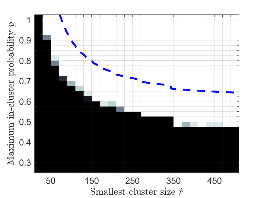
We perform two sets of experiments, one to illustrate the recovery guarantee for dense graphs sampled from the heterogeneous planted cluster model and another to illustrate the guarantee when the noise is sparse. For the dense graph experiments, we fix , and sample graphs from the heterogeneous planted cluster model corresponding to the Bernoulli distributions with probabilities of success given by
for and each and . We choose the number of clusters and distribute the remaining nodes evenly among clusters to ensure that at least one cluster has minimum size. Under this choice of the smallest gap between the in-cluster and between-cluster means occurs when and ; this implies that
For each graph , we call the ADMM algorithm sketched above to solve (5); in the algorithm, we use penalty parameter , stopping tolerance , and maximum number of iterations . We declare the block structure of to be recovered if , where is the solution returned by the ADMM algorithm and is the proposed solution given by (3). Note that Theorem 2.2 implies that we should expect exact recovery (w.h.p.) provided that Figure 1(a) illustrates the empirical success rate for each choice of and , as well as the curve where we use the upper bound to estimate the constant term in (6).
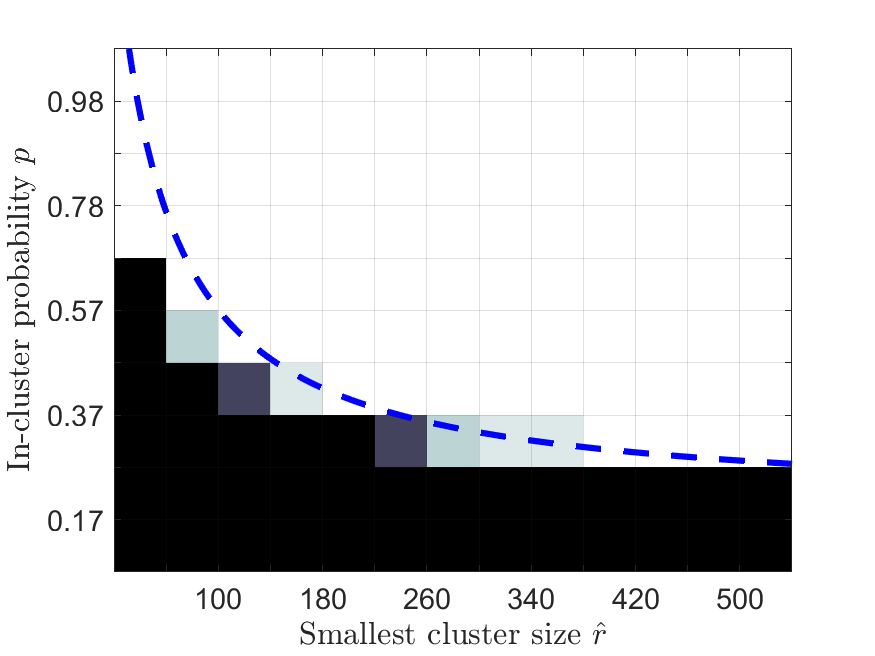
We perform identical experiments for graphs sampled from the homogeneous planted cluster model with sparse noise. In particular, we fix and set . We then sample graphs from the planted cluster model corresponding to the Bernoulli distributions if and if for each and for equally spaced scaling factors between and . As before, we set and distribute the remaining nodes equally amongst the clusters so that the smallest has size and . For each graph , we call the ADMM algorithm to solve (5) (with the same parameters as before) and declare the block structure of recovered if . Theorem 2.2 suggests that we should expect recovery of the cluster structure in the case that
for this particular choice of and . Note that this implies that we have perfect recovery (w.h.p.) for , rather than (as observed in the dense case). Figure 1(b) provides the empirical success rate for each choice of and , as well as the curve . It is clear that we are able to recover significantly smaller clusters under sparse noise than under dense noise, in accordance with (6).
5 Conclusions
We have established theoretical guarantees for graph clustering via a semidefinite relaxation of the densest -disjoint problem. These results add to the growing corpus of evidence that clustering, while intractable in general, is possible if we seek to cluster clusterable data, i.e., data consisting of well-defined and well-separated groups of similar items. Moreover, our results provide further evidence that the barrier can be broken for perfect cluster recovery in approximately sparse graphs and, specifically, that the size of recoverable clusters scales logarithmically with at worst in the special case that all clusters are roughly the same size. Finally, our semidefinite relaxation requires only an estimate of the number of clusters present in the data as input.
Our results suggest several areas of further research. The numerical simulations suggest that our theoretical guarantees may be overly conservative, especially in the dense noise case; further investigation is needed to determine if tighter estimates on the minimum size of clusters efficiently recoverable exist. Moreover, our model assumes clusters are disjoint. This is clearly not met in many practical applications; for example, returning to the social networking realm, users may belong to several overlapping communities. It would be worthwhile to see how our model and recovery guarantees can be modified to address overlapping clusters. Finally, our algorithm for graph clustering requires the solution of a semidefinite program, which may be impractical for even moderately large graphs. For example, the proposed algorithm, based on the ADMM, has per-iteration cost of flops per iteration, primarily to compute the spectral decomposition needed to update . Classical methods based on interior-point methods will scale even more poorly. Efficient, scalable methods for solving this semidefinite relaxation, and semidefinite programming in general, are needed.
Acknowledgements
We are grateful to John Bruer and Joel Tropp for their insights and helpful suggestions. Aleksis Pirinen was supported by a California Institute of Technology Summer Undergraduate Research Fellowship (SURF) using funds provided by Office of Naval Research (ONR) award N000014-11-1002. Brendan Ames was supported by University of Alabama Research Grants RG14678 and RG14838.
Appendix A Proof of Lemma 3.1
We give the full proof of Lemma 3.1 in this appendix.
Proof.
We fix such that and assume without loss of generality that . By the definition (13) of and the triangle inequality, we have
For simplicity, let and . It follows from (14) and our choice of that the th element of , denoted , is given by
It follows from the definition (11) of that
which implies that
Applying (20) with to the right-hand side in the equation above shows that
| (34) |
with high probability, which in turn implies that
with high probability. Similarly, applying (20) with to the sum shows that
for all , with high probability. Finally, we note that
We bound the first term in the sum using (20) with , which establishes that
w.h.p., and note that the second term has upper bound
w.h.p., by a calculation identical to that used to obtain (34). Applying these bounds using the triangle inequality and the union bound over all , we conclude that
| (35) |
with high probability.
We next bound . We have
Appendix B Proof of Proposition 3.2
We next prove Proposition 3.2.
Proof.
We follow the proof of Lemma 4.3 given by Ames (2014). Fix and . It follows from (11) that
for each . Applying (20) with and yields
w.h.p. Moreover, by a similar argument, we have
w.h.p. Combining the above inequalities shows that
w.h.p. Since by (6), this implies that there exists constant such that if
| (37) |
then w.h.p. Applying the union bound over all and shows that each entry of is nonnegative w.h.p. if is chosen to satisfy (37) for all . ∎
Appendix C Proof of Proposition 3.3
Our proof of Proposition 3.3 follows a similar structure to that of Ames (2014, Lemma 4.4).
Appendix D Proof of Lemma 3.2
We next prove Lemma 3.2.
Proof.
We will make repeated use of the following lemma, which specializes the concentration inequality on the spectral norm of a random symmetric matrix with i.i.d. mean zero entries given by Bandeira and van Handel (2016, Corollary 3.12).
Lemma D.1.
Let be a random symmetric matrix with i.i.d. mean zero entries having variance at most and satisfying . Then there exists constant such that
| (38) |
for all .
Proof.
(of Lemma D.1) Corollary 3.12 of Bandeira and van Handel (2016) establishes that for each there exists such that
| (39) |
Here we have substituted the upper bound , in place of in the original statement of Corollary 3.12. Let where is chosen large enough that . In this case, (39) specializes to
This completes the proof. ∎
Before we continue with the derivation of the desired bound on , we note that the entries of all satisfy if we assume that for all ; note that an identical argument establishes the result if we make the weaker assumption that the entries of are bounded with high probability. On the other hand, note that the entries of are not identically distributed (but are independent) since each is sampled according to , where , . However, we know that by our definition of . Moreover, . Thus, we can apply Lemma D.1 to place a bound on . Doing so establishes that (28) holds w.h.p. ∎
Appendix E Proof of Lemma 3.3
We conclude with the following proof of Lemma 3.3.
Proof.
Note that Thus, it remains to bound . To do so, fix . Recall that
Applying (38) with establishes that
w.h.p. On the other hand, Bernstein’s inequality establishes that
w.h.p. Combining these two inequalities using the triangle inequality establishes that
w.h.p. Finally, applying the union bound over all choices of shows that
w.h.p. This establishes that
w.h.p., as required. ∎
References
- Abbe et al. (2016) E. Abbe, A. Bandeira, and G. Hall. Exact recovery in the stochastic block model. IEEE Transactions on Information Theory, 62(1):471–487, 2016.
- Ailon et al. (2013) N. Ailon, Y. Chen, and H. Xu. Breaking the small cluster barrier of graph clustering. In International Conference on Machine Learning, pages 995–1003, 2013.
- Ames (2014) B. Ames. Guaranteed clustering and biclustering via semidefinite programming. Mathematical Programming, 147(1-2):429–465, 2014.
- Ames (2015) B. Ames. Guaranteed recovery of planted cliques and dense subgraphs by convex relaxation. Journal of Optimization Theory and Applications, 167(2):653–675, 2015.
- Ames and Vavasis (2011) B. Ames and S. Vavasis. Nuclear norm minimization for the planted clique and biclique problems. Mathematical programming, 129(1):69–89, 2011.
- Ames and Vavasis (2014) B. Ames and S. Vavasis. Convex optimization for the planted k-disjoint-clique problem. Mathematical Programming, 143(1-2):299–337, 2014.
- Amini and Levina (2018) A. Amini and E. Levina. On semidefinite relaxations for the block model. The Annals of Statistics, 46(1):149–179, 2018.
- Bandeira and van Handel (2016) A. Bandeira and R. van Handel. Sharp nonasymptotic bounds on the norm of random matrices with independent entries. The Annals of Probability, 44(4):2479–2506, 2016.
- Birgin et al. (2000) E. Birgin, M. Martínez, and M. Raydan. Nonmonotone spectral projected gradient methods on convex sets. SIAM Journal on Optimization, 10(4):1196–1211, 2000.
- Boucheron et al. (2013) S. Boucheron, G. Lugosi, and P. Massart. Concentration Inequalities: A Nonasymptotic Theory of Independence. Oxford University Press, 2013.
- Boyd and Vandenberghe (2004) S. Boyd and L. Vandenberghe. Convex Optimization. Cambridge University Press, 2004.
- Cai and Li (2015) T. Cai and X. Li. Robust and computationally feasible community detection in the presence of arbitrary outlier nodes. The Annals of Statistics, 43(3):1027–1059, 2015.
- Chen and Xu (2014) Y. Chen and J. Xu. Statistical-computational phase transitions in planted models: the high-dimensional setting. In International Conference on Machine Learning, pages 244–252, 2014.
- Chen et al. (2014a) Y. Chen, A. Jalali, S. Sanghavi, and H. Xu. Clustering partially observed graphs via convex optimization. The Journal of Machine Learning Research, 15(1):2213–2238, 2014a.
- Chen et al. (2014b) Y. Chen, S. Sanghavi, and H. Xu. Improved graph clustering. IEEE Transactions on Information Theory, 60(10):6440–6455, 2014b.
- Dhillon et al. (2004) I. Dhillon, Y. Guan, and B. Kulis. Kernel k-means: spectral clustering and normalized cuts. In ACM SIGKDD International Conference on Knowledge Discovery and Data Mining, pages 551–556. ACM, 2004.
- Golub and Van Loan (2013) G. Golub and C. Van Loan. Matrix Computations. Johns Hopkins University Press, 4th edition, 2013.
- Guédon and Vershynin (2015) O. Guédon and R. Vershynin. Community detection in sparse networks via Grothendieck’s inequality. Probability Theory and Related Fields, pages 1–25, 2015.
- Hajek et al. (2015) B. Hajek, Y. Wu, and J. Xu. Achieving exact cluster recovery threshold via semidefinite programming. In IEEE International Symposium on Information Theory, pages 1442–1446. IEEE, 2015.
- Holland et al. (1983) P. Holland, K. Laskey, and S. Leinhardt. Stochastic blockmodels: first steps. Social Networks, 5(2):109–137, 1983.
- Jalali et al. (2015) A. Jalali, Q. Han, I. Dumitriu, and M. Fazel. Relative density and exact recovery in heterogeneous stochastic block models. arXiv preprint arXiv:1512.04937, 2015.
- Lei and Rinaldo (2015) J. Lei and A. Rinaldo. Consistency of spectral clustering in stochastic block models. The Annals of Statistics, 43(1):215–237, 2015.
- Leskovec et al. (2008) J. Leskovec, K. Lang, A. Dasgupta, and M. Mahoney. Statistical properties of community structure in large social and information networks. In International Conference on World Wide Web, pages 695–704. ACM, 2008.
- Leskovec et al. (2009) J. Leskovec, K. Lang, A. Dasgupta, and M. Mahoney. Community structure in large networks: natural cluster sizes and the absence of large well-defined clusters. Internet Mathematics, 6(1):29–123, 2009.
- Mathieu and Schudy (2010) C. Mathieu and W. Schudy. Correlation clustering with noisy input. In ACM-SIAM Symposium on Discrete Algorithms, pages 712–728. Society for Industrial and Applied Mathematics, 2010.
- Nellore and Ward (2015) A. Nellore and R. Ward. Recovery guarantees for exemplar-based clustering. Information and Computation, 245:165–180, 2015.
- Ng et al. (2002) A. Ng, M. Jordan, and Y. Weiss. On spectral clustering: analysis and an algorithm. Advances in Neural Information Processing Systems, 2:849–856, 2002.
- Oymak and Hassibi (2011) S. Oymak and B. Hassibi. Finding dense clusters via “low rank + sparse” decomposition. Arxiv preprint arXiv:1104.5186, 2011.
- Peng and Wei (2007) J. Peng and Y. Wei. Approximating k-means-type clustering via semidefinite programming. SIAM Journal on Optimization, 18(1):186–205, 2007.
- Qin and Rohe (2013) T. Qin and K. Rohe. Regularized spectral clustering under the degree-corrected stochastic blockmodel. In Advances in Neural Information Processing Systems, pages 3120–3128, 2013.
- Rohe et al. (2011) K. Rohe, S. Chatterjee, and B. Yu. Spectral clustering and the high-dimensional stochastic blockmodel. The Annals of Statistics, 39(4):1878–1915, 2011.
- Rohe et al. (2014) K. Rohe, T. Qin, and H. Fan. Statistica Sinica, pages 1771–1786, 2014.
- Van Den Berg and Friedlander (2008) E. Van Den Berg and M. Friedlander. Probing the pareto frontier for basis pursuit solutions. SIAM Journal on Scientific Computing, 31(2):890–912, 2008.
- Vinayak et al. (2014) R. Vinayak, S. Oymak, and B. Hassibi. Sharp performance bounds for graph clustering via convex optimization. In IEEE International Conference on Acoustics, Speech and Signal Processing (ICASSP), pages 8297–8301. IEEE, 2014.
- Yan et al. (2017) B. Yan, P. Sarkar, and X. Cheng. Provable estimation of the number of blocks in block models. arXiv preprint arXiv:1705.08580, 2017.
- Zhang and Lu (2011) Y. Zhang and Z. Lu. Penalty decomposition methods for rank minimization. In Advances in Neural Information Processing Systems, pages 46–54, 2011.