Cosmological $N$ -body simulations with suppressed variance

Cosmological

N

-body simulations with suppressed variance–References2016

Raul E. Angulo & Andrew Pontzen ^†^†thanks: rangulo@cefca.es^†^†thanks: a.pontzen@ucl.ac.uk Affiliation: Centro de Estudios de Física del Cosmos de Aragón (CEFCA), Plaza San Juan 1, Planta-2, 44001, Spain. Affiliation: Department of Physics and Astronomy, University College London, Gower Street, London, WC1E 6BT, UK.

Abstract

We present and test a method that dramatically reduces variance arising from the sparse sampling of wavemodes in cosmological simulations. The method uses two simulations which are fixed (the initial Fourier mode amplitudes are fixed to the ensemble average power spectrum) and paired (with initial modes exactly out of phase). We measure the power spectrum, monopole and quadrupole redshift-space correlation functions, halo mass function and reduced bispectrum at $z=1$ . By these measures, predictions from a fixed pair can be as precise on non-linear scales as an average over 50 traditional simulations. The fixing procedure introduces a non-Gaussian correction to the initial conditions; we give an analytic argument showing why the simulations are still able to predict the mean properties of the Gaussian ensemble. We anticipate that the method will drive down the computational time requirements for accurate large-scale explorations of galaxy bias and clustering statistics, enabling more precise comparisons with theoretical models, and facilitating the use of numerical simulations in cosmological data interpretation.

Keywords:

cosmology: dark matter – cosmology: large-scale structure of the Universe – cosmology: theory – methods: numerical

August 24, 2026

1 Introduction

Numerical simulations are an essential tool for cosmology, especially for interpreting observational surveys (see Kuhlen et al. 2012 for a review). They can be deployed to probe the impact of a given cosmological ingredient (Baldi et al., 2014, e.g.), create virtual galaxy populations (Overzier et al., 2009, e.g.), check and develop analytic treatments for structure formation (Carlson et al., 2009, e.g.), and understand systematic and statistical errors in cosmological measurements (Manera et al., 2015, e.g.). In the future, simulations could even be used to constrain cosmological parameters (Angulo & Hilbert, 2015).

However, a limitation for all the above applications is the sparse sampling of Fourier modes due to the finite extent of the simulation box. A given cosmological simulation is initialised to a particular realisation of a Gaussian random field. The power spectrum of the realisation, $\hat{P}^{\mathrm{\,L}}(k)$ , therefore differs from the ensemble mean power spectrum, $P^{\mathrm{\,L}}(k)$ . Given a box large enough to capture all physical effects (Bagla et al., 2009), the largest-scale modes are still poorly sampled. This, together with the non-linear coupling of small and large scales, implies that several-Gpc size boxes generate statistical errors which limit inferences on $100$ or even $10\,\mathrm{Mpc}$ scales.

This under-sampling effect is closely connected to (though, owing to the non-linear evolution, not precisely the same as) observational cosmic variance. In the observational case, the finite volume that can be achieved by a given survey constitutes an irreducible source of uncertainty. On the other hand the computational variance can be strongly suppressed, at least in principle, until it is smaller than the cosmic variance and other sources of error. This is usually achieved by simulating huge cosmological volumes (Rasera et al., 2014, e.g.) or a large number of realisations (Takahashi et al., 2009, e.g.). Finite computing resources then generate a tension between the need for large volumes and for high resolution (the latter is required to better resolve the distribution of individual galaxies and their internal structure). Even as supercomputing facilities expand, the tension is becoming more acute as surveys probe larger scales and constrain the statistics of fluctuations to greater precision. For instance, reaching 1% accuracy over the whole range of scales to be probed by Euclid would require the simulation of $\sim 10^{5}$ Gpc³.

In this Letter we propose and test a method to suppress the effect of box variance drastically. We will show that with just two simulations we can achieve the accuracy delivered by tens to hundreds of traditional simulations at the same scale, depending on the particular problem in hand. Briefly, the two simulations:

1.

use a fixed input power spectrum, meaning that we enforce $\hat{P}^{\mathrm{\,L}}=P^{\mathrm{\,L}}$ when generating the initial conditions;
2.

are paired, so that a hierarchy of effects due to chance phase correlations can be cancelled (Pontzen et al., 2016).

The first condition destroys the statistical Gaussianity of the input field which, at first sight, would seem to limit the usefulness of the approach (Neyrinck & Yang, 2013, see also). However we will demonstrate empirically and analytically that, by all measures explored here, the non-Gaussian corrections have a negligible effect on ensemble mean clustering statistics.

This Letter is set out as follows. In Section 2 we implement and test our method. In particular, we quantify its performance by comparing predictions with those from an ensemble of 300 independent simulations. We develop an analytic understanding of why the method works in Section 3. Finally, in Section 4 we present our conclusions.

2 Comparison with an ensemble of simulations

2.1 Numerical Simulations

Refer to caption — Figure 1: The probability density function of non-linear overdensities in spheres of radius $8\,h^{-1}{\rm Mpc}$ , as measured in the fixed simulations (orange lines) and in an ensemble of Gaussian simulations (grey lines), at the starting redshift, $z=9$ . The blue line and red circles show the mean of the respective cases, as indicated by the legend.

All simulations considered in this Letter contain $1024^{3}$ particles of mass $1.7\times 10^{12}\,h^{-1}M_{\odot}$ inside a box of side $L=3\,h^{-1}{\rm Gpc}$ . The initial particle positions are computed from an input linear density field $\delta^{\mathrm{L}}$ using 2LPT. The simulation particles are then evolved under self-gravity with a COLA algorithm (Tassev et al., 2013) using 10 steps from $z=9$ to $z=1$ . The cosmological parameters assumed correspond to those of the Millennium series (Springel, 2005): $\Omega_{m}=0.25$ , $\sigma_{8}=0.9$ , and $h=0.73$ .

The COLA algorithm is an approximate $N$ -body method, in the sense that the orbits inside high density regions are not properly integrated. However, the non-linear evolution of intermediate and large scales is accurately captured (Howlett et al., 2015; Koda et al., 2016), at a fraction of the computational cost of a traditional $N$ -body simulation. This enables the rapid simulation of extremely large volumes, which in turn allows very precise calculations of different statistics that serve as a benchmark for the performance of our method. The total volume of our reference ensemble is $8100\,h^{-1}\,\rm{Gpc}^{3}$ ; more details are given in Chaves-Montero et al. (in prep).

The only difference between the ensemble of simulations and the pair of fixed simulations is in the input fields $\delta^{\mathrm{L}}(\boldsymbol{\mathbf{x}})$ . Because of the finite box size, the Fourier modes for the field are quantised; we write

\delta^{\mathrm{L}}(\boldsymbol{\mathbf{x}})\equiv\sum_{i}e^{i\boldsymbol{\mathbf{k}}_{i}\cdot\boldsymbol{\mathbf{x}}}\delta^{\mathrm{L}}_{i}\textrm{,}

(1)

where $i$ indexes the possible modes and $\delta^{\mathrm{L}}_{i}$ is the Fourier amplitude for the mode at wavevector $\boldsymbol{\mathbf{k}}_{i}$ . We can choose the indexing such that $\boldsymbol{\mathbf{k}}_{-i}=-\boldsymbol{\mathbf{k}}_{i}$ ; note that, for the field $\delta^{\mathrm{L}}(\boldsymbol{\mathbf{x}})$ to remain real, $\delta_{i}^{\mathrm{L}*}=\delta^{\mathrm{L}}_{-i}$ .

The reference ensemble of 300 simulations consists of boxes each with $\delta^{\mathrm{L}}_{i}$ s drawn from a Gaussian, zero-mean probability distribution function (pdf). Decomposed into the the magnitude $|\delta^{\mathrm{L}}_{i}|$ and phase $\theta_{i}\equiv\arg\delta^{\mathrm{L}}_{i}$ , the pdf for each independent mode $i$ is given by

\mathrm{Pr}_{g}\left(\left|\delta^{\mathrm{L}}_{i}\right|,\theta_{i}\right)\equiv\frac{|\delta^{\mathrm{L}}_{i}|}{\pi P_{i}}\exp\left(-\frac{\left|\delta^{\mathrm{L}}_{i}\right|^{2}}{P_{i}}\right),

(2)

where $P_{i}$ is the discrete version of the power spectrum $P(k)$ . In the fixed-power approach, the pdf for mode $i$ is instead given by

\mathrm{Pr}_{f}\left(\left|\delta^{\mathrm{L}}_{i}\right|,\theta_{i}\right)\equiv\frac{1}{2\pi}\delta_{D}\left(\left|\delta^{\mathrm{L}}_{i}\right|-\sqrt{P_{i}}\right),

(3)

where $\delta_{D}$ indicates the Dirac delta-function. One can sample from $\mathrm{Pr}_{f}$ straightforwardly by setting

\delta^{\mathrm{L}}_{i}=\sqrt{P_{i}}\exp\left(i\theta_{i}\right),

(4)

with $\theta_{i}$ drawn with uniform probability between $0$ and $2\pi$ , and $\theta_{-i}=-\theta_{i}$ . The second of the pair of simulations is then generated by transforming $\theta_{i}\to\pi+\theta_{i}$ (Pontzen et al., 2016).

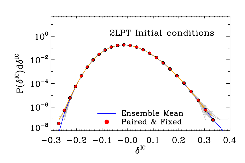
Sampling from $\mathrm{Pr}_{f}$ results in an ensemble that is not equivalent to sampling from $\mathrm{Pr}_{g}$ . However, $\mathrm{Pr}_{f}$ can stand in place of $\mathrm{Pr}_{g}$ for many practical calculations (the analytic justification is discussed in Section 3). We verified that, despite the fixed amplitudes, the one-point input overdensity pdf in real space, $\delta^{\mathrm{L}}(\boldsymbol{\mathbf{x}})$ , is still a Gaussian deviate owing to the central limit theorem. Furthermore, Fig. 1 shows the distribution of overdensities in the initial conditions at $z=9$ , $\delta^{IC}$ , averaged over spheres of $8\,h^{-1}{\rm Mpc}$ radius for a subset of traditional simulations (grey lines) and the two paired-and-fixed (orange lines; these overlap almost perfectly). The corresponding pdf for the combined volume of the two paired-and-fixed simulations is shown by the red dots. There is excellent agreement between this characterisation of the density fields of traditional and fixed simulations, with both following a near-Gaussian distribution. The mild skewness (which also agrees between the cases) arises from the 2LPT particle displacements.

2.2 Results

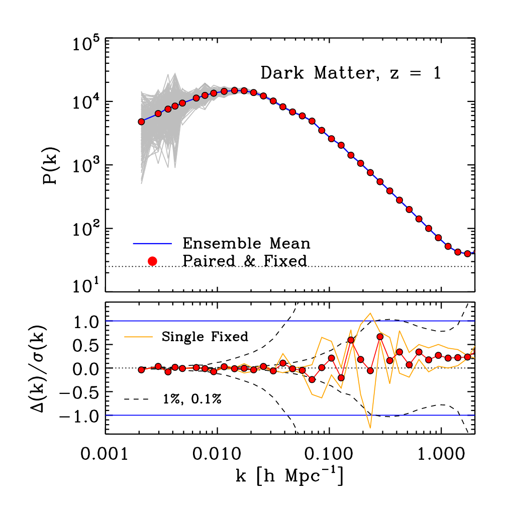
Fig. 2 shows the dark matter power spectrum measured from the $z=1$ outputs. In the top panel, the results of the fixed pair (red circles) are indistinguishable from the traditional ensemble mean (blue line) over all the scales plotted, confirming that the approach correctly predicts the ensemble average power spectrum in linear and in non-linear regimes.

The bottom panel shows deviations with respect to the ensemble mean, in units of the standard deviation of the ensemble, $\sigma(k)=(\langle\hat{P}^{\mathrm{\,NL}}(k)^{2}\rangle-\langle\hat{P}^{\mathrm{\,NL}}(k)\rangle^{2})^{1/2}$ . On scales where evolution is linear (approximately $k<0.03\,h{\rm Mpc^{-1}}$ ) the fixed simulations should exactly coincide with linear theory by construction. As expected, the measured power spectrum agrees with the ensemble mean to an accuracy limited only by the statistical errors of the latter, $\sigma(k)/\sqrt{300}\lesssim 2\%$ of $P(k)$ . At larger $k$ , non-linear effects — which depend not only on the initial amplitude of Fourier modes but also on phases — become important. Accordingly, the power spectrum of the two individual fixed simulations (orange lines) drift away from the exact mean. However the leading order deviations from the ensemble mean are equal and opposite in sign (Pontzen et al., 2016) between the pair of fixed simulations, so that their average (red dots) has a reduced r.m.s. error much below $1\%$ ( $0.27\sigma$ over the range $0.03<k\,h{\rm Mpc^{-1}}<1$ ). The accuracy of our pair of fixed simulations by this measure is approximately equivalent to averaging over 14 traditional simulations, allowing for a factor 7 reduction in computer time. In particular, the technique suppresses statistical errors on all scales to the point where they are smaller than the impact of numerical parameters (Schneider et al., 2016).

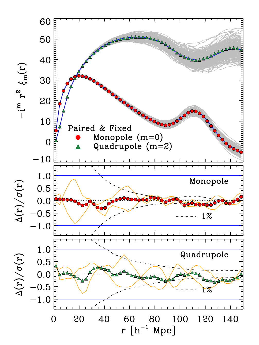
In Fig. 3 we show that the high accuracy of the method also holds in redshift space. In this figure we plot the monopole (red circles) and quadrupole (green triangles) terms of an expansion of the 2D correlation function in terms of Legendre polynomials. Predictions from the pair of fixed simulations again agree well with the ensemble mean. The same pattern persists where the individual fixed simulations perform best on large scales, while on smaller scales the pairing leads to a substantial cancellation of remaining errors. The overall technique yields a precise prediction for the non-linear correlation function, reaching a $2\%$ accuracy over the whole range of scales investigated (in particular around the baryonic acoustic oscillation peak, whose shape and location is currently driving large simulation campaigns). With traditional ensemble-average techniques, achieving this accuracy would require around $50$ simulations of $3\,h^{-1}{\rm Gpc}$ box size.

Having established the accuracy of our simulations for predicting two-point statistics, we now turn to higher-order clustering. The bispectrum is defined (in the limit that the box size is infinite) by

B(k_{1},k_{2},\theta)\,\delta_{D}(\boldsymbol{\mathbf{k}}_{1}+\boldsymbol{\mathbf{k}}_{2}+\boldsymbol{\mathbf{k}}_{3})=\langle\delta^{\mathrm{NL}}(\boldsymbol{\mathbf{k}}_{1})\delta^{\mathrm{NL}}(\boldsymbol{\mathbf{k}}_{2})\delta^{\mathrm{NL}}(\boldsymbol{\mathbf{k}}_{3})\rangle\textrm{,}

(5)

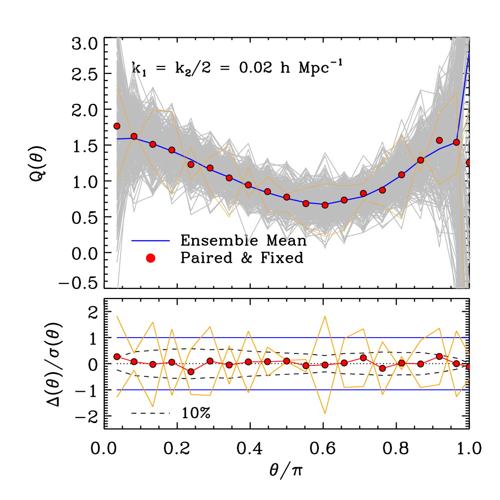
where $\delta^{\mathrm{NL}}(\boldsymbol{\mathbf{k}})$ is the Fourier transform of the non-linear evolved overdensity. We have assumed statistical isotropy in writing $B$ as a function of $\theta$ , the angle between the $\boldsymbol{\mathbf{k_{1}}}$ and $\boldsymbol{\mathbf{k_{2}}}$ vectors, and statistical homogeneity imposes the Dirac-delta dependence on the left-hand-side. We particularly consider the case where $k_{1}=0.02\,h^{-1}{\rm Mpc}$ and $k_{2}=0.04\,h^{-1}{\rm Mpc}$ to capture the onset of non-linearity, and plot the reduced bispectrum

Q(\theta)=\frac{\hat{B}(k_{1},k_{2},\theta)}{\hat{P}^{\mathrm{\,NL}}(k_{1})\hat{P}^{\mathrm{\,NL}}(k_{2})+\hat{P}^{\mathrm{\,NL}}(k_{1})\hat{P}^{\mathrm{\,NL}}(k_{3})+\hat{P}^{\mathrm{\,NL}}(k_{2})\hat{P}^{\mathrm{\,NL}}(k_{3})},

(6)

where $\hat{B}$ is the estimated bispectrum from a simulation. The definition of $Q(\theta)$ divides out much of the sensitivity to the power spectrum realisation. Accordingly, when we plot this quantity in Fig. 4, each of the two individual fixed simulations exhibit fluctuations of an amplitude comparable to that in traditional realisations. However, the pairing procedure cancels the leading-order contribution to these fluctuations because they have odd parity in the input linear density field. Therefore the final estimate from the pair of fixed simulations has an r.m.s. deviation from the ensemble average of only $0.14\sigma$ over all $\theta$ . Reaching this accuracy with traditional simulations would again require averaging over 50 (as opposed to two) realisations.

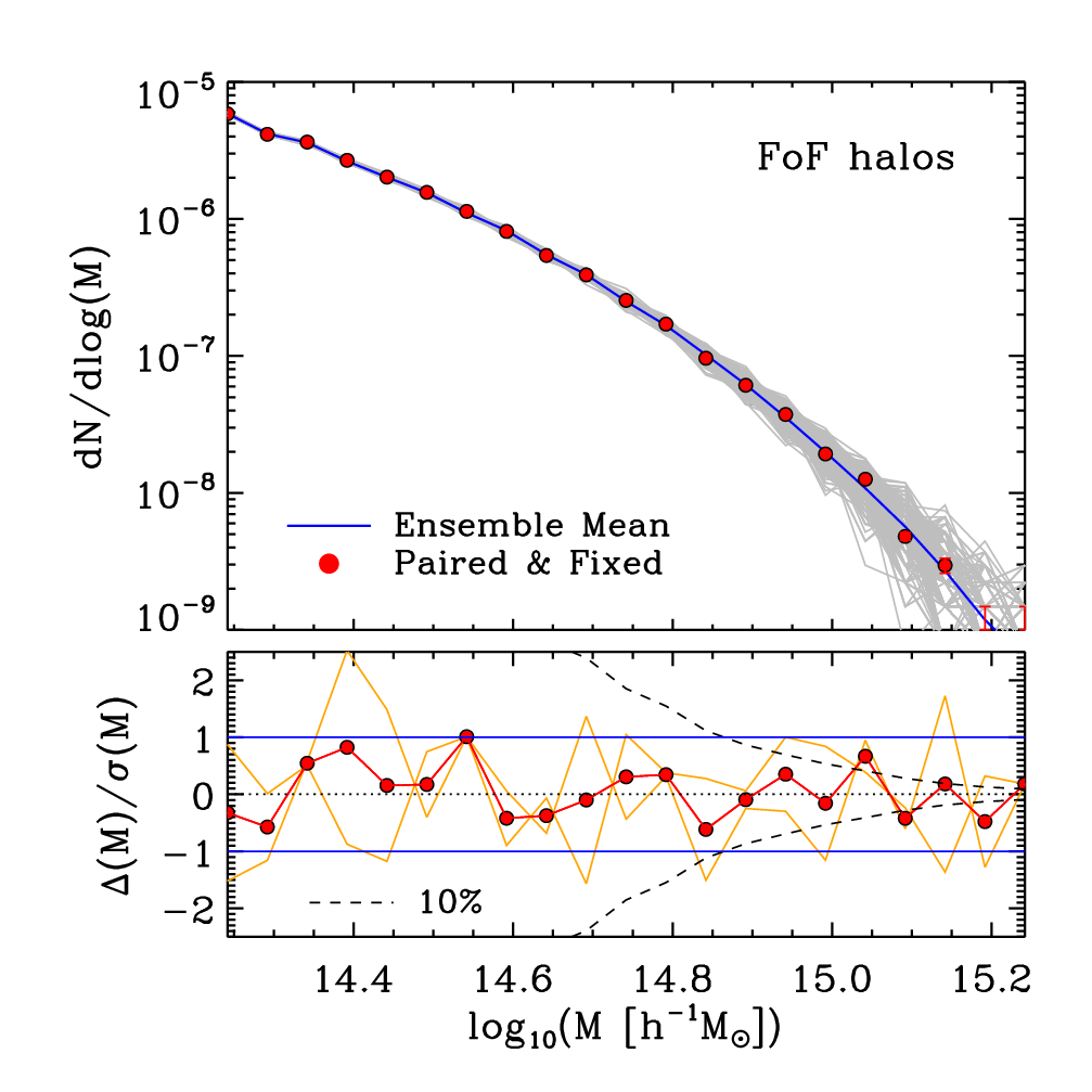
As discussed in Koda et al. (2016), the COLA $N$ -body algorithm does not resolve the internal structure of halos but nonetheless predicts accurate mass functions for the overall population. Therefore we can meaningfully test the abundance of collapsed objects. In Fig. 5 we show the mass function of dark matter halos identified using a Friends-of-Friends algorithm (Davis et al., 1985) with a linking length set to $l=0.2$ . We find the same qualitative picture as in previous plots and statistics, although with slightly less striking noise suppression. The new method produces results with suppressed fluctuations relative to two Gaussian simulations, with strong cancellations between the pair. The average r.m.s. error is $0.47\sigma$ , roughly the level expected from four simulations randomly picked from the traditional ensemble.

3 Analytic exploration

In the previous Section we showed that paired-and-fixed simulations are able to predict the average properties of a traditional ensemble. We will now explore the technique from an analytic perspective. The pairing approach has recently been introduced and discussed elsewhere (Pontzen et al., 2016, see particularly section II.C) and so our focus is on the power spectrum fixing. Sampling from the $\hat{P}(k)$ -fixed pdf $\mathrm{Pr}_{f}$ , defined by equation (3), is not equivalent to sampling from the true Gaussian $\mathrm{Pr}_{g}$ , equation (2). The aim of this Section is therefore to motivate more precisely why $\mathrm{Pr}_{f}$ has reproduced the ensemble average results of $\mathrm{Pr}_{g}$ .

Expectation values of any $n$ -point expression with respect to either $\mathrm{Pr}_{f}$ or $\mathrm{Pr}_{g}$ will be denoted by $\langle\delta_{i_{1}}\cdots\delta_{i_{n}}\rangle_{f}$ and $\langle\delta_{i_{1}}\cdots\delta_{i_{n}}\rangle_{g}$ respectively. In the case of the fixed distribution, we can use expression (4) to write that

\langle\delta^{\mathrm{L}}_{i_{1}}\cdots\delta^{\mathrm{L}}_{i_{n}}\rangle_{f}=\frac{\sqrt{P_{i_{1}}\cdots P_{i_{n}}}}{(2\pi)^{N}}\int_{0}^{2\pi}\mathrm{d}^{N}\theta\,\exp\left(i\theta_{i_{1}}+\cdots+i\theta_{i_{n}}\right)\textrm{,}

(7)

where the integral is over the possible $\theta$ values for all $N$ modes.

For $n=1$ the single phase factor $\exp(i\theta_{1})$ averages to zero, and consequently $\langle\delta^{\mathrm{L}}_{i}\rangle_{g}=\langle\delta^{\mathrm{L}}_{i}\rangle_{f}=0$ . This result extends to any $n$ -point correlation for $n$ odd; we therefore need only consider the even- $n$ cases further.

For $n=2$ , the properties of the two pdfs are indistinguishable:

\langle\delta^{\mathrm{L}}_{i}\delta^{\mathrm{L}}_{j}\rangle_{f}=\langle\delta^{\mathrm{L}}_{i}\delta^{\mathrm{L}}_{j}\rangle_{g}=\delta_{i,-j}P_{i}\textrm{,}

(8)

where $\delta_{i,-j}$ is the Kronecker delta equal to $1$ when $i=-j$ and $0$ otherwise, and there is no sum implied over repeated indices. The Gaussian result is standard, and the fixed result is obtained by seeing that when $i\neq-j$ , the $i$ and $j$ phase integrals in equation (7) evaluate to zero. For $n=4$ , the Gaussian result follows by Wick’s theorem:

\langle\delta^{\mathrm{L}}_{i}\delta^{\mathrm{L}}_{j}\delta^{\mathrm{L}}_{k}\delta^{\mathrm{L}}_{l}\rangle_{g}=\delta_{i,-j}\delta_{k,-l}P_{i}P_{k}+\delta_{i,-k}\delta_{j,-l}P_{i}P_{j}+\delta_{i,-l}\delta_{j,-k}P_{i}P_{j}\textrm{.}

(9)

The fixed result, again obtained through use of (7) is similar to the Gaussian case because indices must be “paired up” for their phase integrals to be non-vanishing. The only difference arises in the case where $\delta_{i}\delta_{j}\delta_{k}\delta_{l}=|\delta_{i}|^{4}$ ; here, the Gaussian result is $\langle|\delta^{\mathrm{L}}_{i}|^{4}\rangle_{g}=3P_{i}^{2}$ but in the fixed case we find that $\langle|\delta^{\mathrm{L}}_{i}|^{4}\rangle_{f}=P_{i}^{2}$ . Overall the result is therefore

\langle\delta^{\mathrm{L}}_{i}\delta^{\mathrm{L}}_{j}\delta^{\mathrm{L}}_{k}\delta^{\mathrm{L}}_{l}\rangle_{f}=\langle\delta^{\mathrm{L}}_{i}\delta^{\mathrm{L}}_{j}\delta^{\mathrm{L}}_{k}\delta^{\mathrm{L}}_{l}\rangle_{g}-2\left(\delta_{ij}\delta_{kl}\delta_{i,-k}+\delta_{ik}\delta_{jl}\delta_{i,-j}+\delta_{il}\delta_{jk}\delta_{i,-j}\right)P_{i}^{2}\textrm{,}

(10)

assuming that we have $P_{0}=0$ (otherwise a further term is necessary to divide the correction by $3$ in the $i=j=k=l=0$ case).

The correction (10) is consistent with how the power spectrum of a fixed realisation must have zero variance:

\left\langle\left(|\delta^{\mathrm{L}}_{i}|^{2}-P_{i}\right)^{2}\right\rangle_{f}=\left\langle\left(|\delta^{\mathrm{L}}_{i}|^{2}-P_{i}\right)^{2}\right\rangle_{g}-2P_{i}^{2}=0\textrm{.}

(11)

Evidently there is a dramatic difference — intentionally so — between fixed and Gaussian statistics: in the linear regime, the fixed $P(k)$ approach reproduces the ensemble mean with no variance. While this also means that the input trispectrum is unavoidably non-Gaussian by equation (10), the correction only appears when all indices always take the same value (up to sign). We can now explain why most measures of the output non-linear density field are extremely insensitive to this change.

The non-linear density field can be written in standard perturbation theory (Bernardeau et al., 2002, SPT, e.g.) as

\delta^{\mathrm{NL}}_{i}=\delta^{\mathrm{L}}_{i}+\sum_{jk}F^{(2)}_{ijk}\delta^{\mathrm{L}}_{j}\delta^{\mathrm{L}}_{k}+\sum_{ijkl}F^{(3)}_{ijkl}\delta^{\mathrm{L}}_{j}\delta^{\mathrm{L}}_{k}\delta^{\mathrm{L}}_{l}+\cdots

(12)

where $F^{(n)}_{\cdots}$ for $n=2,3,\cdots$ are the discretised version of the SPT kernels which in turn are homogeneous, degree-zero, continuous functions of the wavevectors. As a concrete example of an observable correlation in this formalism, we can consider the one-loop SPT non-linear power spectrum with Gaussian statistics:

	$\displaystyle P^{\mathrm{NL,g}}_{i}$	$\displaystyle\equiv\langle\delta^{\mathrm{NL}}_{i}\delta^{\mathrm{NL}}_{-i}\rangle_{g}\simeq P_{i}+\sum_{jklm}\left(F^{(2)}_{ijk}F^{(2)}_{-i,lm}+2\delta_{i,-j}F^{(3)}_{iklm}\right)\times$
		$\displaystyle\left(\delta_{j,-k}\delta_{l,-m}P_{j}P_{l}+\delta_{j,-l}\delta_{k,-m}P_{j}P_{k}+\delta_{j,-m}\delta_{k,-l}P_{j}P_{k}\right)\textrm{.}$		(13)

Momentum conservation implicit in the $F^{(n)}_{\cdots}$ s and explicit in the Kronecker deltas eliminate three of the summations, so that the overall summation is over just one index. Therefore the magnitude of the one-loop terms scales proportionally to $N_{k}P(k)$ where $k$ is a characteristic scale and $N_{k}$ is the number of modes around that scale (as defined by the range of modes over which the relevant $F$ is large). In a continuum limit (i.e. as the box size $L\to\infty$ ), $N_{k}$ turns into the appropriate Fourier-space volume. These simple scaling behaviours are assured by the degree-zero homogeneity of the $F^{(n)}$ functions.

In the fixed case, expression (13) must be corrected by using relation (10), giving

\displaystyle P^{\mathrm{NL,f}}_{i}\simeq P^{\mathrm{NL,g}}_{i}-12F^{(3)}_{i,-i,i,-i}P_{i}^{2}-2\sum_{j}F^{(2)}_{ijj}F^{(2)}_{-i,-j,-j}P_{j}^{2}\textrm{,}

(14)

which is valid at one-loop order for the case $\boldsymbol{\mathbf{k}}_{i}\neq 0$ . Here most of the Kronecker deltas have already been summed out; the remaining summation, by momentum conservation in $F^{(2)}$ , only has a contribution at the index $j$ with $\boldsymbol{\mathbf{k}}_{j}=\boldsymbol{\mathbf{k}}_{i}/2$ . The overall contribution of the correction (14) is therefore suppressed relative to the physical terms in equation (13) by $\mathcal{O}(N_{k})$ .

For the bispectrum with Gaussian statistics, we have

	$\displaystyle B^{g}_{ijk}$	$\displaystyle\equiv\langle\delta^{\mathrm{NL}}_{i}\delta^{\mathrm{NL}}_{j}\delta^{\mathrm{NL}}_{k}\rangle_{g}$
		$\displaystyle\simeq 2F^{(2)}_{i,-j,-k}P_{j}P_{k}+\delta_{j,-k}\sum_{l}F^{(2)}_{il,-l}P_{j}P_{l}+\textrm{cyc. perms in }ijk$		(15)

to one-loop order. The second term contributes only for $\boldsymbol{\mathbf{k}}_{i}=0$ . The correction is now

B^{f}_{ijk}=B^{g}_{ijk}-4F^{(2)}_{i,j,-j}P_{j}^{2}\delta_{jk}-2F^{(2)}_{i,-j,-j}P_{j}^{2}\delta_{jk}-\textrm{cyc. perms in }ijk\textrm{,}

(16)

and is non-zero only in the case where $\boldsymbol{\mathbf{k}}_{j}=\boldsymbol{\mathbf{k}}_{k}=-\boldsymbol{\mathbf{k}}_{i}/2$ or $\boldsymbol{\mathbf{k}}_{i}=0$ (or a cyclic permutation of those configurations). All other bispectra are unaffected by the changed statistics at this order.

For higher order perturbation theory (or higher- $n$ correlations) the overall pattern established here will remain: the linear $n$ -point correction term (10) will always involve at least one extra Kronecker delta relative to the physical part (9). For observable correlations, this implies that either the effect is diluted by a power of a large factor $N_{k}$ (as in the case of the one-loop power spectrum) or plays a role only in a measure-zero part of the continuous function being studied (as in the case of the one-loop bispectrum). The intentionally-reduced power spectrum variance (11) falls into the latter category, since it is only the diagonal part of the full covariance that is altered.

4 Conclusions

In this Letter we have explored a new method to suppress the impact of under-sampling Fourier modes in simulations.

By fixing the initial amplitude of Fourier modes to the ensemble mean, variance has been eliminated on linear scales. In the non-linear regime, the suppression is imperfect because phase-correlation effects begin to impact on the evolved amplitudes. However by also pairing the simulation with a phase-reversed counterpart (Pontzen et al., 2016) we can average away the leading-order imperfections of this type; fluctuations about the ensemble mean are then near-identical in magnitude but opposite in sign. Residual noise could be reduced arbitrarily by considering an ensemble of paired-and-fixed simulations with different realisations of the initial random phases.

We have tested the non-linear dark matter power spectrum, the multipoles of the redshift-space correlation function, the reduced bispectrum and the halo mass function. In all cases, the method is unbiased (up to the accuracy of our comparison ensemble averages) and strongly suppresses unwanted variance. These tests were carried out with a suite of 300 COLA simulations at $z=1$ . The analytic arguments of Section 3 suggest that the accuracy of the results should be maintained to all redshifts. Similarly, we do not expect results to change when using more accurate integration methods than COLA, especially since small-scale gravitational collapse are largely insensitive to large-scale correlations. All these points deserve systematic investigation in future.

Paired simulations can be used with purely Gaussian initial conditions if desired, retaining many of the small-scale benefits we have discussed. Conversely, single unpaired simulations with fixed amplitudes can be used, retaining the large-scale benefits. Whenever fixing is applied, the ensemble statistics are not strictly Gaussian. The local one-point pdf is, however, unaffected (Figure 1) and furthermore our numerical results directly show that a variety of statistics attain the correct, unbiased ensemble mean value. We gave an analytic discussion of why the non-Gaussianity does not impinge, arguing that the errors are either strongly suppressed by the large density of modes or, in other cases, affect only a measure-zero set of correlations. Fixing the power spectrum does need to be approached with care but our results underline that it can be a valuable technique.

Straightforward applications are in any comparison to analytic models, in characterisation of the performance of data modelling, in emulators and in development of fitting functions for non-linear statistics. It will be particularly valuable to couple the technique to high-resolution simulations incorporating baryonic effects to measure galaxy bias, free of the usual difficulties of large-scale variance. Furthermore the method could be used in combination with rescaling techniques to quickly predict galaxy clustering statistics as a function of cosmological parameters (Angulo & White, 2010). All these are crucial steps towards a comprehensive exploitation of upcoming survey data.

Acknowledgements

We would like to thank Jonás Chavez-Montero for providing us with access to the ensemble of COLA simulations. We thank the Lorentz Center and the organisers of the “Computational Cosmology” workshop where this study was initiated, and Oliver Hahn, Carlos Hernandez-Monteagudo, Aseem Paranjape, Hiranya Peiris, Anže Slosar, and Matteo Viel for helpful discussions. REA acknowledges support from AYA2015-66211-C2-2. AP is supported by the Royal Society.

References

Angulo & Hilbert (2015) Angulo R. E., Hilbert S., 2015, MNRAS, 448, 364
Angulo & White (2010) Angulo R. E., White S. D. M., 2010, MNRAS, 401, 1796
Bagla et al. (2009) Bagla J. S., Prasad J., Khandai N., 2009, MNRAS, 395, 918
Baldi et al. (2014) Baldi M., Villaescusa-Navarro F., Viel M., Puchwein E., Springel V., Moscardini L., 2014, MNRAS, 440, 75
Bernardeau et al. (2002) Bernardeau F., Colombi S., Gaztañaga E., Scoccimarro R., 2002, Phys. Rep., 367, 1
Carlson et al. (2009) Carlson J., White M., Padmanabhan N., 2009, Phys. Rev. D, 80, 043531
Davis et al. (1985) Davis M., Efstathiou G., Frenk C. S., White S. D. M., 1985, ApJ, 292, 371
Howlett et al. (2015) Howlett C., Manera M., Percival W. J., 2015, Astronomy and Computing, 12, 109
Koda et al. (2016) Koda J., Blake C., Beutler F., Kazin E., Marin F., 2016, MNRAS, 459, 2118
Kuhlen et al. (2012) Kuhlen M., Vogelsberger M., Angulo R., 2012, Physics of the Dark Universe, 1, 50
Manera et al. (2015) Manera M. et al., 2015, MNRAS, 447, 437
Neyrinck & Yang (2013) Neyrinck M. C., Yang L. F., 2013, MNRAS, 433, 1628
Overzier et al. (2009) Overzier R. A., Guo Q., Kauffmann G., De Lucia G., Bouwens R., Lemson G., 2009, MNRAS, 394, 577
Pontzen et al. (2016) Pontzen A., Slosar A. c. v., Roth N., Peiris H. V., 2016, Phys. Rev. D, 93, 103519
Rasera et al. (2014) Rasera Y., Corasaniti P.-S., Alimi J.-M., Bouillot V., Reverdy V., Balmès I., 2014, MNRAS, 440, 1420
Schneider et al. (2016) Schneider A. et al., 2016, J. Cosmology Astropart. Phys, 4, 047
Springel (2005) Springel V., 2005, MNRAS, 364, 1105
Takahashi et al. (2009) Takahashi R. et al., 2009, ApJ, 700, 479
Tassev et al. (2013) Tassev S., Zaldarriaga M., Eisenstein D. J., 2013, J. Cosmology Astropart. Phys, 6, 036

Cosmological NN-body simulations with suppressed variance