An optimal single-electron charge qubit for solid-state double quantum dots

The effective potential in an experimental DQD system can be found using density functional theory [11, 12] and will be a complex function of all three spatial coordinates $x,y,z$. By careful design, the dynamics in two of the directions $y$ and $z$ can be confined to the lowest energy subbands so that only the potential in the $x$ direction, $V_{DQD}(x,t)$ needs be considered. For example in a GaAs/AlGaAs heterostructure, the $z$ direction is the growth direction and modulation doping can be used to create a triangular quantum well in that direction with subband energies two orders of magnitude larger than either $\varepsilon$ or $\Delta$. In the $y$ direction, parabolic confinement with energies an order of magnitude larger than $\varepsilon$ or $\Delta$ can be produced either by etching [13], fabricating a thin gate wrapping the conducting channel [14, 15] or using split-gates [16]. In order to create a DQD potential in the $x$ direction, gates [17, 18, 19, 20] or etching [21, 13] can also be used.

The aim is to create a potential $V_{DQD}(x,t)$ that has two minima separated by a tunnel barrier. A convenient potential that has this property and is defined by four parameters $z_{0}$, $z_{2}$ and $w_{1}$, $w_{2}$ is given by

This form for $V_{DQD}$ allows us to control both the depth of the dots and the barrier between them directly, using the parameters $z_{0}$ and $z_{2}$, respectively. For a specific set of parameters, this static potential will define a value for $\Delta$ which is the energy difference between the bonding ground state $E_{B}$ and the antibonding first excited state $E_{AB}$. Detuning is introduced by adding a linear stark shift of the form

By comparing the dependences of $E_{B}$ and $E_{AB}$ on $V_{\mathrm{slope}}$ with the expected dependences from LSM Hamiltonian we can define the detuning parameter for $V_{DQD}$ through a linear relation $\varepsilon=\lambda V_{\mathrm{slope}}$ with $\lambda$ being constant. We find this linear relationship holds with an accuracy of one part in $10^{6}$ across the range of required values of $\varepsilon$ for single-qubit operations. The total potential is $V_{\mathrm{tot}}(x)=V_{\mathrm{DQD}}(x)+V_{\mathrm{bias}}(x)$ and Fig. 1 (a) shows this potential at three different detunings.

The DQD dynamics under time-dependent detuning will be given by the TDSE

with

Time dependence is included in Eq. 5 by varying the potential slope with time: $V_{\mathrm{slope}}(t)$. An example plot of the energies of the two lowest instantaneous solutions (the bonding and antibonding states) as function of $V_{\mathrm{slope}}$ is shown in Fig. 1 (b).

Analytic solutions to the TDSE in Eq. 6 can only be found in special cases. In this paper we solve Eq. 5 numerically using a GPU-accelerated version of the staggered-leapfrog method [22, 23] (see App. A, App. B).

Here and throughout the paper we use the parameter values: $w_{1}=130\text{nm}$, $w_{2}=240\text{nm}$, $z_{0}=0.865\text{meV}$, $z_{2}=6.92\text{meV}$ so that $\mathit{\Delta}=12\mu\text{eV}$, and the linear coefficient $\lambda=0.42254$. The values are chosen to be in agreement with the experiments [1, 24], however, our conclusions are applicable to any DQD system and do not depend on the specific choice of parameter values. We have also tested various non-symmetric potentials with the two dots having different sizes, but in all the cases the general conclusions were the same as for the symmetric potential of Eq. 3.

We denote the optimal qubit basis for the potential $V_{DQD}(x)$ as the two states $\psi_{0}(x)$ and $\psi_{1}(x)$. In order to make measurement of arbitrary qubit states $\psi(x)=\alpha\psi_{0}(x)+\beta\psi_{1}(x)$ as straightforward as possible these basis states would ideally be maximally localised in the left and right dots respectively. This is because experimentally, it is possible to measure the probability that an electron will tunnel out of a quantum dot and this probability is in turn proportional to the probability that the electron is in that dot. Also, in order to avoid complex transient oscillations, the qubit basis states should be linear combinations of the two lowest instantaneous eigenstates of the DQD system. For the Hamiltonian in Eq. 6, the two lowest eigenstates are the instantaneous bonding and anti-bonding states $\psi_{\varepsilon}^{B}(x)$ and $\psi_{\varepsilon}^{AB}(x)$ for detuning $\varepsilon$. Hence, the qubit basis states will be,

where $\alpha_{\varepsilon}$ and $\beta_{\varepsilon}$ are real variables, $\alpha_{\varepsilon}^{2}+\beta_{\varepsilon}^{2}=1$ and $\alpha_{\varepsilon}$ is chosen such that the integral

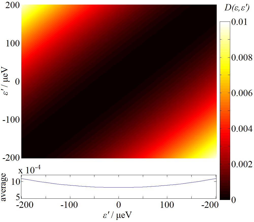
is maximised. Readout would then simply be a matter of determining which dot the electron wave function collapsed into. However, for a given pulse sequence these qubit basis states are time-dependent and cannot easily be compared to qubits with different detunings $\varepsilon$. Therefore, it is preferable to define a stationary qubit basis, independent of $\varepsilon$. Optimal basis states of this type should have the greatest overlap with $R_{\varepsilon}(x)$ and $L_{\varepsilon}(x)$ for all detunings. Fig. 2 shows a correlation function $D(\varepsilon,\varepsilon^{\prime})$ that will be a minimum when this condition is met:

The detuning range is chosen such that the fidelity

is always $\geqslant 99\%$ for all values of $\varepsilon$, where, $\phi_{\varepsilon}(x)=a_{\varepsilon}R_{0}(x)+b_{\varepsilon}L_{0}(x)$, $(a_{\varepsilon}$,$b_{\varepsilon}$) is the corresponding bonding solution to $\hat{H}_{\mathrm{{eff}}}$ in Eq. 2, and a similar measure is performed for the anti-bonding state. As expected, $D(\varepsilon,\varepsilon^{\prime})$ is smallest between states where the difference in detunings is small. However, as we want to apply large biases across the double dot system, the best qubit states are the ones where $D(\varepsilon,\varepsilon^{\prime})$ is minimised over the entire domain $\varepsilon-\varepsilon^{\prime}$.

Using this criterion, we find that the best choice of states from which to build the qubits of the system are the bonding and anti-bonding states at zero detuning. By parity inversion symmetry when $V_{\mathrm{bias}}(x,t)=0$, if $x\to-x$ then $R_{0}(x)\to L_{0}(x)$ with $\psi_{0}^{B}(x)\to\psi_{0}^{B}(x)$ and $\psi_{0}^{AB}(x)\to-\psi_{0}^{AB}(x)$ so the coefficients $\alpha_{0}=\beta_{0}=1/\sqrt{2}$. Therefore, our optimal charge qubits are defined as

These qubits are optimal in the sense that they have the greatest overlap with the maximally localised states in Eqs. 7 and 8 across the specified range of detunings. These states are not fully localised as the probability density of $\psi_{0}(x)$ in the left dot is non-zero, and similarly for $\psi_{1}(x)$ in the right dot (Fig. 3). However, these are the states which maximise the sum of probabilities (red colour plot in Fig. 3) and further localisation of the states would include higher-energy states which would not obey the ideal LSM Hamiltonian in Eq. 2 which we want to model.

The qubit we have established here, as a linear combination of bonding and anti-bonding states at zero detuning, is well defined in any DQD system including potentials that are not spatially symmetric. Since, in the definition, there is no reference to the underlying effective potential of the DQD, this qubit is also well defined for an experimental system.

It is important to be able to initialise a qubit in a well defined state, preferably $\psi_{0}(x)$ or $\psi_{1}(x)$. For a generic experiment involving a charge qubit, we would expect the initial state of the electron to be the ground state of Eq. 6. This is not one of the qubit states so, in order to initialise the electron in the qubit state, we need to perform a rotation. The exact parameters required for this procedure will vary for different detunings $\varepsilon$, for example, at certain detunings, the ground state wave function will be closer to one of the qubit basis states, but the general procedure reported here is the same.

To rotate the wave function from the initial eigenstate to the qubit $\psi_{0}(x)$ state, we applied a trapezoidal pulse, as shown in Fig. 4 (a). We performed a sweep of pulse lengths $t_{p}$ and detuning amplitudes $A=\varepsilon$ and calculated the distance

between the resultant state $\psi(x)$ and the qubit state $\psi_{0}(x)$. For an initial static detuning $V_{\mathrm{slope}}(0)=0.06508\text{meV}$, corresponding to $\varepsilon=27.5\mu\text{eV}$ we found that this distance was minimized when $t_{p}=537$ps and $A=11.5\mu$eV with an accuracy of $S<10^{-5}$.

In experiment, these parameters can be found by applying the same pulse to two distinct systems: one initialised in the ground state, and the other in the first excited state, then performing a sweep over pulse amplitudes and lengths and finding those which maximise the summed probability of finding the former state in the right and the latter one in the left dot, respectively, in agreement with Fig. 3.

Having prepared the qubit in the state $\psi_{0}(x)$, we will now demonstrate how to perform a $\sigma_{x}$ rotation through an angle $\vartheta$ on the Bloch sphere. When the response time of the quantum system is negligible, ie. $\tau=0$, this rotation is achieved by switching the detuning to zero. For $\varepsilon=0$, the Hamiltonian in Eq. 2 takes the form

so that the rotation in Eq. 15 becomes

Once the qubit has rotated by the desired angle, the detuning is returned to its original value. With finite rise times, this process translates to a trapezoidal pulse shape similar to the one used for the state preparation in Sec. III.1.

Significantly, the trapezoidal pulse is not able to produce a pure $\sigma_{x}$ rotation. To show this, we initiated the qubit in the $\psi_{0}(x)$ state and swept $A$ in the range described in Sec. II.2 and $t_{p}$ from 0 to 1000 ps (enough for all the rotations to make at least one full circle on the Bloch sphere). After choosing the values for which the oscillation amplitude, defined as the difference between the maximum and the minimum probabilities of finding the qubit in the other state $\psi_{1}(x)$, was the highest, we used these optimal pulse parameters on the set of three mutually orthogonal states from Sec. III to map the pulse to the rotation:

where $\vec{n}_{\mathrm{trans}}$ is the axis of a transient rotation due to the finite rise and, for the tunnelling energy and pulse rise times we have chosen, $\kappa=0.029$ and $\vartheta_{\mathrm{trans}}=\pi-0.10$. Importantly, the transient rotation axis $\vec{n}_{\mathrm{trans}}$ is not aligned with the $\sigma_{z}$ axis so these rotations do not commute and cannot be translated into a pure $\sigma_{x}$ rotation. With the trapezoidal pulse, we were therefore unable to find any values of $A$ and $t_{p}$ for which the qubit experienced a pure $\sigma_{x}$ rotation on the Bloch sphere.

The solution, inspired by the spin-echo technique [31], was to use the modified pulse shown in Fig. 4 (b). The counter-detuning, of amplitude $\bar{A}^{\prime}$, applied at the beginning and end of the pulse was introduced to correct the transient rotation generated by the finite rise time. We swept the parameters $A^{\prime},\bar{A}^{\prime}$ and measured the oscillation amplitude as we vary $t_{p}$. The resulting amplitudes are shown in Fig. 5. For a high fidelity $\sigma_{x}$ rotation, the state should oscillate between $\psi_{0}(x)$ and $\psi_{1}(x)$, so that the amplitude of the oscillation should equal 1. We found the region with the highest oscillation amplitude and performed more detailed sweeps around it, as shown in Fig. 6. Testing the results on the same set of three mutually orthogonal states, we were able to generate a qubit rotation of the form

where $\vartheta_{0}=-1.416$ and $\kappa^{\prime}=-0.031$ for $\bar{A}^{\prime}=-167.4\mu$eV and $A^{\prime}=16.5\mu$eV. This represents a $\sigma_{x}$ rotation of angle $\vartheta_{0}+\kappa^{\prime}(t-4\tau)$ together with an additional $\pi$ rotation around the $\sigma_{z}$ axis. This additional rotation can be corrected either by performing the qubit operation twice or by relabelling the qubit states $\psi_{0}(x)\to\psi_{0}(x),\psi_{1}(x)\to-\psi_{1}(x)$.

Establishing this type of rotation for an experimental DQD is straightforward. Using the technique for readout of the optimal qubit described in Sec. IV we can relate the measured probability with the qubit coefficients, and therefore identify values of $A^{\prime}$ and $\bar{A^{\prime}}$ that give the largest oscillation amplitude. Once the values of $A^{\prime}$ and $\bar{A}^{\prime}$ are determined, the parameters $\vartheta$ and $\kappa^{\prime}$ can be found by measuring the resulting probability for the shortest pulse (for $t_{p}=4\tau$) and the oscillation frequency, respectively.

We applied a similar procedure to find optimal pulse parameters for performing a $\sigma_{z}$ rotation on the Bloch sphere. Again, the trapezoidal pulse was not able to generate a pure $\sigma_{z}$ rotation. To show this, we initialised the qubit in the $\psi_{0}(x)$ state and performed a parameter sweep for a trapezoidal pulse with a maximum possible detuning of $A_{\mathrm{max}}=200\mu$eV, i.e. within the range given in Fig. 2. Again, transient rotations dominated these operations and it was not possible to obtain a rotation where the oscillation amplitude between the qubits was not less than $25\%$ (a high fidelity $\sigma_{z}$ rotation only introduces a phase difference, thus there should be no change in the amplitude). Therefore, we again tried the modified pulse from Sec. III.2 (Fig. 4 (b)) and used the sweep from Fig. 5, this time focusing on the regions with the lowest amplitude. As a result, we were able to successfully find a qubit operation where the oscillation amplitude was small (less than 0.003). Once again, we mapped out the operation using the set of three mutually orthogonal eigenstates and found a rotation around the $\sigma_{z}$ axis of the Bloch sphere with the form:

For our system, $\vartheta_{0}^{\prime}=2.658$ and $\kappa^{\prime\prime}=0.359$ with pulse detunings $\bar{A}=-181.2\mu$eV and $A=177.0\mu$eV. It is worth noting that, as opposed to standard Ramsey interferometry-type experiments, this $\sigma_{z}$ rotation is achieved using a single pulse without the need for additional $\pi$ pulses around the perpendicular ($\sigma_{x}$) axis [32].

Similarly to the approach discussed in Sec. III.2, the values for $A^{\prime}$ and $\bar{A}^{\prime}$ can be found by relating the measured probability with the qubit coefficients, as described in Sec. IV.

References

- [1] T. Hayashi, T. Fujisawa, H. D. Cheong, Y. H. Jeong, and Y. Hirayama, Phys. Rev. Lett. 91, 226804 (2003).
- [2] T. Fujisawa, T. Hayashi, and S. Sasaki, Rep. Prog. Phys. 69, 759 (2006).
- [3] J. R. Petta, A. C. Johnson, J. M. Taylor, E. A. Laird, A. Yacoby, M. D. Lukin, C. M. Marcus, M. P. Hanson, and A. C. Gossard, Science 309, 2180 (2005).
- [4] K. D. Petersson, J. R. Petta, H. Lu, and A. C. Gossard, Phys. Rev. Lett. 105, 246804 (2010).
- [5] M. Veldhorst, J. C. C. Hwang, C. H. Yang, A. W. Leenstra, B. de Ronde, J. P. Dehollain, J. T. Muhonen, F. E. Hudson, K. M. Itoh, A. Morello, and A. S. Dzurak, Nature Nanotech. 9, 981 (2014).
- [6] S. Lloyd, Science 261, 1569 (1993).
- [7] D. P. DiVincenzo, Fortschritte der Physik 48, 771 (2000).
- [8] Y. Dovzhenko, J. Stehlik, K. D. Petersson, J. R. Petta, H. Lu, and A. C. Gossard, Phys. Rev. B 84, 161302 (2011).
- [9] M. Kataoka, M. R. Astley, A. L. Thorn, D. K. L. Oi, C. H. W. Barnes, C. J. B. Ford, D. Anderson, G. A. C. Jones, I. Farrer, D. A. Ritchie, and M. Pepper, Phys. Rev. Lett. 102, 156801 (2009).
- [10] A. Rossi, T. Ferrus, G. J. Podd, and D. A. Williams, Appl. Phys. Lett. 97, 223506 (2010).
- [11] E. T. Owen and C. H. W. Barnes, (2015), arXiv:1509.02457 .
- [12] M. Stopa, Phys. Rev. B 54, 13767 (1996).
- [13] T. Ferrus, A. Rossi, M. Tanner, G. Podd, P. Chapman, and D. A. Williams, New J. Phys. 13, 103012 (2011).
- [14] Y. K. D. Hisamoto, T. Kaga and E. Takeda, IEEE Electron Device Letters 11, 36 (1990).
- [15] B. Voisin, V.-H. Nguyen, J. Renard, X. Jehl, S. Barraud, F. Triozon, M. Vinet, I. Duchemin, Y.-M. Niquet, S. de Franceschi, and M. Sanquer, Nano Lett. 14, 2094 (2014).
- [16] B. J. van Wees, H. van Houten, C. W. J. Beenakker, J. G. Williamson, L. P. Kouwenhoven, D. van der Marel, and C. T. Foxon, Phys. Rev. Lett. 60, 848 (1988).
- [17] T. Fujisawa, W. G. van der Wiel, and L. P. Kouwenhoven, Physica E 73, 413 (2000).
- [18] S. Gardelis, C. G. Smith, J. Cooper, D. A. Ritchie, E. H. Linfield, Y. Jin, and M. Pepper, Phys. Rev. B 67, 073302 (2003).
- [19] W. H. Lim, H. Huebl, L. H. W. van Beveren, S. Rubanov, P. G. Spizzirri, S. J. Angus, R. G. Clark, and A. S. Dzurak, Appl. Phys. Lett. 94 (2009).
- [20] N. Mason, M. J. Biercuk, and C. M. Marcus, Science 303, 655 (2004).
- [21] D. Wei, H.-O. Li, G. Cao, G. Luo, Z.-X. Zheng, T. Tu, M. Xiao, G.-C. Guo, H.-W. Jiang, and G.-P. Guo, Sci. Rep. 3 (2013).
- [22] A. Askar and A. S. Cakmak, J. Chem. Phys. 68, 2794 (1978).
- [23] E. T. Owen, M. C. Dean, and C. H. W. Barnes, Phys. Rev. A 85, 022319 (2012).
- [24] T. Fujisawa, T. Hayashi, H. D. Cheong, Y. H. Jeong, and Y. Hirayama, Physica E 21, 1046 (2004).
- [25] In practical implementations, measurement of the probability is taken at the end of the pulse where decoherence does not yet affect the amplitude. In our model, there is no explicit inclusion of coherent mechanisms and so, the specific time at which measurement is performed is less critical .
- [26] F. H. L. Koppens, C. Buizert, K. J. Tielrooij, I. T. Vink, K. C. Nowack, T. Meunier, L. P. Kouwenhoven, and L. M. K. Vandersypen, Nature 442, 766 (2006).
- [27] L. Landau, Physics of the Soviet Union 2, 46 (1932).
- [28] C. Zener, Proc. R. Soc. London A 137, 696 (1932).
- [29] E. C. G. Stueckelberg, Helvetica Physica Acta 5, 369 (1932).
- [30] S. Foletti, H. Bluhm, D. Mahalu, V. Umansky, and A. Yacoby, Nature Phys. 5, 903 (2009).
- [31] E. L. Hahn, Phys. Rev. 80, 580 (1950).
- [32] H. Y. Carr and E. M. Purcell, Phys. Rev. 94, 630 (1954).
- [33] J. J. V. Maestri, R. H. Landau, and M. J. Paez, Am. J. Phys. 69, 1113 (2000).
- [34] P. B. Visscher, Comput. Phys. 5, 596 (1991).
- [35] C. Leforestier, R. H. Bisseling, C. Cerjan, M. D. Feit, R. Friesner, A. Guldberg, A. Hammerich, G. Jolicard, W. Karrlein, H.-D. Meyer, N. Lipkin, O. Roncero, and R. Kosloff, J. Comp. Phys. 94, 59 (1991).
- [36] A. Munshi, ed., The OpenCL Specification, Version: 2.0 (Khronos OpenCL Working Group, 2014).