Traffic regulation via controlled speed limitThanks: This research was supported by the NSF grant CNS 1446715 and by KI-Net ”Kinetic description of emerging challenges in multiscale problems of natural sciences” - NSF grant # 1107444
Abstract
We study an optimal control problem for traffic regulation via variable speed limit. The traffic flow dynamics is described with the Lighthill-Whitham-Richards (LWR) model with Newell-Daganzo flux function. We aim at minimizing the quadratic error to a desired outflow, given an inflow on a single road. We first provide existence of a minimizer and compute analytically the cost functional
variations due to needle-like variation in the control policy. Then, we compare three strategies: instantaneous policy; random exploration of control space; steepest descent using numerical expression of gradient. We show that the gradient technique is able to achieve a cost within 10% of random exploration minimum with better computational performances.
Keywords: Traffic problems, Optimal control problem, Variable speed limit
AMS subject classification:90B20, 35L65, 49J20
1 Introduction
In this paper, we study an optimal control problem for traffic flow on a single road using a variable speed limit. The first traffic flow models on a single road of infinite length using a non-linear scalar hyperbolic partial differential equation (PDE) are due to Lighthill and Whitham [31] and, independently, Richards [33], which in the 1950s proposed a fluid dynamic model to describe traffic flow. Later on, the model was extended to networks [18] and started to be used to control and optimize traffic flow on roads. In the last decade, several authors studied optimization and control of conservation laws and several papers proposed different approaches to optimization of hyperbolic PDEs, see [5, 17, 19, 22, 29, 34, 35] and references therein. These techniques were then employed to optimize traffic flow through, for example, inflow regulation [11], ramp-metering [32] and variable speed limit [20]. We focus on the last approach, where the control is given by the maximal speed allowed on the road. Notice that also the engineering literature presents a wealth of approaches [1, 2, 9, 10, 12, 14, 23, 24, 25, 26, 27, 28, 36], but mostly in the time discrete setting. In [1, 2] a dynamic feedback control law is employed to compute variable speed limits using a discrete macroscopic model. Instead, [23, 24, 25] use model predictive control (MPC) to optimally coordinate variable speed limits for freeway traffic with the aim of suppressing shock waves.
In this paper, we address the speed limit problem on a single road.
The control variable is the maximal allowed velocity, which may vary in time but we assume
to be of bounded total variation, and
we aim at tracking a given target outgoing flow. More precisely, the main goal is to minimize the quadratic difference between the achieved outflow and the given target outflow.
Mathematically the problem is very hard, because of the delays in the effect of the control variable (speed limit). In fact, the Link Entering Time (LET) , which represents the entering time of the car exiting the road at time see (7),
depends on the given inflow and the control policy on the whole
time interval . Moreover, the input-output map is defined in terms of LET,
thus the achieved outflow at time depends on the control variable on the whole interval .
Due to the complexity of the problem, in this article we restrict the problem to free flow conditions. Notice that this assumption is not too restrictive. Indeed, if the road is initially in free flow, then it will keep the free flow condition due to properties of the LWR model, see [8, Lemma 1].
After formulating the optimal control problem, we consider needle-like variations for the control policy
as used in the classical Pontryagin Maximum Principle [7].
We are able to derive an analytical expression of the one-sided variation of the cost,
corresponding to needle-like variations of the control policy, using fine properties
of functions with bounded variation. In particular the one-sided variations depend
on the sign of the control variation and involves integrals w.r.t. to the distributional derivative
of the solution as a measure, see (10).
This allows us to prove Lipschitz continuity of the cost
functional in the space of bounded variation function and prove existence of a solution.
Afterwards, we define three different techniques to solve numerically this problem.
- •
Instantaneous Policy (IP). We design a closed-loop policy, which depends only on the instantaneous density at road exit. More precisely, we choose the speed limit which gives the nearest outflow to the desired one.
- •
Random Exploration (RE). It uses time discretization and random binary tree search of the control space to find the best maximal velocity profile.
- •
Gradient Descent Method (GDM). It consists in approximating numerically the gradient of the cost functional using (10) combined with a steepest descent method.
We compare the three approaches on two test cases: constant desired outflow and sinusoidal inflow; sinusoidal desired outflow and inflow. In both cases RE provides the best control policy, however GDM performs within 10% of best RE result with a computational cost of around 15% of RE. On the other side, IP performs poorly with respect to the RE, but with a very low computational cost. Notice that, in some cases, IP may be the only practical policy, while GDM represents a valid approach also for real-time control, due to good performances and reasonable computational costs. Moreover, control policies provided by RE may have too large total variation to be of practical use.
The paper is organized as follows: section 2 gives the description of the traffic flow model and of the optimal control problem. Moreover, the existence of
a solution is proved. In section 3, the three different approaches to find control policies
are described. Then in section 4, these techniques are implemented on two test cases. Final remarks and future work are discussed in section 5.
2 Mathematical model
In this section, we introduce a mathematical framework for the speed regulation problem. The traffic dynamics is based on the classical Lighthil-Whitham-Richards (LWR) model ([31, 33]), while the optimization problem will seek minimizers of quadratic distance to an assigned outflow.
2.1 Traffic flow modeling
We consider the LWR model on a single road of length to describe the traffic dynamics. The evolution in time of the car density is described by a Cauchy problem for scalar conservation law with time dependent maximal speed :
| (1) |
where with the maximal car density. In the transportation literature the graph of the flux function (in our case for a fixed ) is commonly referred to as the fundamental diagram. Throughout the paper, we focus on the Newell - Daganzo - type ([13]) fundamental diagrams, see Figure 1b. The speed takes value on a bounded interval , thus the flux function is given by
| (2) |
with representing the maximal speed, see Figure 1a.
Notice that the flow is increasing up to a critical density
and then decreasing. The interval is referred to as
the free flow zone, while is referred to
as the congested flow zone.
The problem we consider is the following. Given an inflow ,
we want to track a fixed outflow on a time horizon , by acting on the time-dependent maximal velocity
A maximal velocity function
is called a control policy.
It is easy to see that a road in free flow can become congested
only because of the outflow regulation with shocks moving backward,
see [8, Lemma 2.3]. Since we assume Neumann boundary conditions at the road exit,
the traffic will always remain in free flow, i.e.
for every
Given the inflow function , we consider the Initial Boundary Value Problem
with assigned flow boundary condition on the left and Neumann boundary condition (flow ) on the right:
| (3) |
We denote by the space of scalar functions of bounded variations and by the total variation, see [6] for details. For any scalar function we denote by its right (respectively left) limit at . We further assume the following:
Hypothesis 1
There exists and such that and
Under this assumption, we have:
Proposition 1
Proof. Let be a sequence of piecewise constant functions converging to in and satisfying For each , by standard properties of Initial Boundary Value Problems for conservation laws [15], there exists a unique BV entropy solution to (3) with . Notice that the left flow condition is equivalent to the boundary condition: . From [8, Lemma 2.3] and the Neumann boundary condition on the right, we get that , thus by maximum principle it holds:
Let us now estimate the total variation of the solution . Since it solves a scalar conservation laws, the total variation does not increase in time due to dynamics on . Notice that changes in will not increase the total variation of inside the road (i.e. on ). The total variation of increases only because of new waves generated by changes in the inflow. Using the boundary condition , we can estimate the total variation in space of caused by time variation of In, respectively time variation of , by , respectively . Finally we get:
By Helly’s Theorem (see [6, Theorem 2.4]) there exists a subsequence converging in to a limit .
By Lipschitz continuity of the flux and dominated convergence we get that
converges
in to .
Passing to the limit in the weak formulation
(where and
) we have that is a weak entropic solution.
We can pass to the limit also in the left boundary condition because
this is equivalent to and
is bounded from below.
Finally is a solution to (3).
The standard Kružhkov entropy condition [30] ensures uniqueness of the solution.
Since , we have that
has bounded variation and satisfies (6).
To simplify notation,
we further make the following assumptions:
Hypothesis 2
We assume Hypothesis 1 and the following:
Given a control policy , we can define a Link Entering Time (LET) function representing the entering time for a car exiting the road at time . The function depends on the control policy , but for simplicity we will write when the policy is clear from the context. Notice that LET is defined only for time greater than a given , the exit time of the car entering the road at time , see Figure 2.
Note that satisfies and, for each :
| (7) |
Such is unique, due to the hypothesis From the identity
we get the following:
Lemma 1
Given a control policy , the function is a Lipschitz continuous function, with Lipschitz constant .
Recalling the definition of outflow of the solution given in (4), we get:
Proposition 2
The input-output flow map of the Initial Boundary Value Problem (briefly IBVP) (3) is given by
| (8) |
Proof. Thanks to Proposition 1, the solution to the IBVP (3) satisfies , thus solves a conservation law linear in . Indeed the Newell-Daganzo flow is linear in the free flow zone. Therefore, no shock is produced inside the domain and characteristics are defined for all times. In particular the value of is constant along characteristics. The characteristic exiting the domain at time enters the domain from the boundary at time . Therefore we get . From (4) we get the desired conclusion.
Remark 1
This map is highly non-linear with respect to the control policy due to the definition of . Hence, the classical techniques of linear control cannot be applied. Moreover, such formulation clearly shows how delays enter the input-output flow map. The effect of the control at time on the outflow depends on the choice of on the time interval , because of the presence of the LET map in formula (8).
2.2 Optimal control problem
We are now ready to define formally the problem of outflow tracking.
Problem 1
Remark 2
We use the same positive extreme values for both the inflow and the target outflow for simplicity of notation only.
Remark 3
In the simple case where all the parameters are constant in time, i.e. do not depend on time, the problem has a a trivial solution which is realizing .
2.3 Cost variation as function of control policy variation
In this section we estimate the variation of the cost with respect to the perturbations of the control policy . This computation will allow to prove continuous dependence of the solution from the control policy.
We first fix the notation for integrals of function with respect to Radon measures.
Definition 2.1
Let be a -function and a Radon measure. We define
where is the decomposition of into its continuous11 1 We recall that any Radon measure on can be decomposed into its continuous (AC+Cantor) and Dirac parts, as a consequence of the Lebesgue decomposition Theorem, see e.g. [16] . and Dirac parts.
We now compute the variation in the cost produced by needle-like variation in the control policy , i.e. variation of the value of on small intervals of the type in the same spirit as the needle variations of Pontryagin Maximum Principle [7].
Definition 2.2
Consider and a time such that and . Let , be sufficiently small such that and . We define a needle-like variation of , corresponding to , and by setting if and otherwise, see Figure 3.
Lemma 2
Remark 4
Notice that the condition implies that the outflow , depends only on the inflow and not on the initial density If such condition is not satisfied, the perturbation given by has a comparable effect on , but it needs to be estimated in two parts: one with respect to and one with respect to with being such that
The condition means that the perturbation has influence on the whole outflow in the interval . If this is not satisfied, then the influence of the perturbation is stopped at , hence the variation is smaller.
Proof.
Let be defined according to (7) and an outflow according to (8).
For simplicity we assume that has a constant value
on , the general case holding because of properties of functions.
We define and to be the unique value satisfying
to be the unique value satisfying
and , hence . Notice that . We also define the function
| (11) |
Remark that is a decreasing function, with , , and .
We denote with the outflow, the LET (see (7)) and the density for the policy . Clearly, we have for and for .
To compute the variation, we distinguish four time intervals:
, , and see Figure 4.
The variation of the cost in the first interval can be directly computed
as function of the velocity variation, while in the other intervals
the delays in the outflow formula (8) will render
the computation more involved.
We denote with the contributions to in the four intervals and estimate them separately.
CASE 1 : .
Let , then
and .
We have:
| (12) |
Substituting the expressions for the outflows we get
Dividing the first integral in two parts and making the change of variable
After simple algebraic manipulation we get:
Taking the limit as , we get:
hence
thus
CASE 2 : . If then and . After decomposing as done for in (12) and plugging in the expression of the outflows, we have
| (13) |
Applying the change of variable (see (11)), it holds
Notice that this change of variable is justified by Lemma 3 of the Appendix. Using Lemma 4 of the Appendix, we get:
CASE 3 : . If then and
After decomposing as done for in (12) and plugging in the expression of the outflows, we get
Observe that and , then
| (14) |
thus
CASE 4 : . If then we compute
and
We decompose as done with in (12), plug in the expression of the outflows, and use the equality . The, denoting , we have
By passing to the limit, we get
Proposition 3
For every and , the functional is Lipschitz continuous on endowed with the norm .
Proof. Let , . Then is in and can be approximated by piecewise constant functions. This means the can be approximated in by needle-like variations as in Lemma 2. The right-hand side of (10) is uniformly bounded (since and with uniformly bounded variation). Therefore we conclude that for some .
This allows to prove the following existence result.
Proposition 4
Problem 1 admits a solution.
3 Control policies
In this section, we define three control policies for the time-dependent maximal speed . The first, called the instantaneous policy (IP), is defined by minimizing the instantaneous contribution for the cost at each time. We will show that such control policy does not provide a global minimizer, due to delays in the control effect on the cost for the Problem 1. In particular, due to the bound the instantaneous minimization may induce a larger cost at subsequent times. Then, we introduce a second control policy, called random exploration (RE) policy. Such policy uses a random path along a binary tree, which correspond the upper and lower bounds for , i.e. and . Lastly, a third control policy is based on a gradient method descent (GDM) and uses the expression given by Lemma 2 to numerically find the gradient of the cost.
3.1 Instantaneous policy
Definition 3.1
Consider Problem 1. Define the instantaneous policy as follows:
| (15) |
where the projection is the function
| (16) |
Notice that this would be the optimal choice if and would be constant, see Remark 3. The instantaneous policy can also be written directly in terms of the input-output map defined in Proposition 2. As we will show later, the instantaneous policy is not optimal in general, i.e., it does not provide an optimal solution for Problem 1. Clearly, it provides the solution in the case of sufficiently small and sufficiently big so that the projection operator reduces to the identity, i.e., for all times. Indeed, in this case the output coincides with , hence the cost is zero.
3.2 Random exploration policy
The random exploration policy is defined as follows:
Definition 3.2
Given the extreme values for the maximal speed, and , and a time step , the random exploration policy draws sequences of velocities from the set corresponding to control policy values on the intervals .
Notice that maximal speeds according to this algorithm can be generated for all times, independently of the corresponding solution, in contrast to the instantaneous policy which is based on the maximal speed at previous times. We will use numerical optimization to choose the best among the generated random policies, showing in particular that the instantaneous policy is not optimal in general.
3.3 Gradient method
We use needle-like variations and the analytical expression in (10) to numerically compute one-sided variations of the cost. We consider such variations as estimates of the gradient of the cost in . More precisely, we give the following definition.
Definition 3.3
We will show that the gradient method gives very good results compared to the other policies taking into account the computational complexity.
4 Numerical simulations
In this section we show the numerical results obtained by implementing the policies described in section 3. The numerical algorithm for all the approaches is composed of two steps:
- 1.
- 2.
Numerical solution for the optimal control problem, i.e., computation of the maximal speed using the instantaneous control, random exploration policy and gradient descent.
Let and be the fixed space and time steps, and set , the cell interfaces such that the computational cell is given by The center of the cell is denoted by for at each time step for We fix the number of space points and the finite time horizon. We now describe in detail the two steps.
4.1 Godunov scheme for hyperbolic PDEs
The Godunov scheme is a first order scheme, based on exact solution to Riemann problems. Given the cell average of in the cell at time is defined as
| (17) |
Then, the Godunov scheme consists of two main steps:
- 1.
Solve the Riemann problem at each cell interface with initial data .
- 2.
Compute the cell averages at time in each computational cell and obtain .
Remark 5
Waves in two neighboring cells do not intersect before if the following CFL (Courant-Friedrichs-Lewy) condition holds:
| (18) |
The Godunov scheme can be expressed in conservative form as:
| (19) |
where is the maximal speed at time . Additionally, is the Godunov numerical flux that in general has the following expression:
| (20) |
For clarity, we included as an argument for the Godunov scheme the maximal velocity so that the dependence of the scheme on the optimal control could be explicit.
4.2 Velocity policies
The next step in the algorithm consists of computing a control policy that can be used in the Godunov scheme with the different approaches introduced in section 3. In particular, for the instantaneous policy approach we compute the velocity at each time step using the instantaneous outgoing flux. Instead, using the other two approaches, the RE and the GDM, we compute beforehand the value of the velocity at each time step and then use it to solve the conservation law with the Godunov scheme.
4.2.1 Instantaneous policy
We follow the control policy described in section 3.1 for the instantaneous control. At each time step, the velocity is computed using the following formula:
| (21) |
4.2.2 Random exploration policy
To compute for each time step the value of the velocity, we use a randomized path on a binary tree, see Figure 5. With such technique, we obtain several sequences of possible velocities. For each sequence the velocities are used to compute the fluxes for the numerical simulations. We then choose the sequence that minimizes the cost.
Remark 6
Notice that the control policy RE may have a very large variation, not respecting the bounds given in Problem 1. Therefore the found control policies may not be feasible. However, we implement this technique for comparison with the results and performances obtained by the GDM.
4.2.3 Gradient descent method
We first numerically compute one-sided variations of the cost using (10). Then, we use the classical gradient descent method [3] to find the optimal control strategy and to compute the optimal velocity that fits the given outflow profile, as described in Algorithm 1.
4.3 Simulations
We set the following parameters: Moreover, the input flux at the boundary of the domain is given by . We choose two different target fluxes and . The initial condition is a constant density We use oscillating inflows to represent variations in typical inflow of urban or highway networks at the 24h time scale.
4.3.1 Test I: Constant Outflow
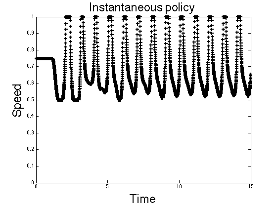
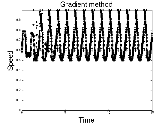
In Figure 6, we show the time-varying speed obtained by using the instantaneous policy (left) and by using the gradient descent method (right). In each case, we notice that due to the oscillating input signal the control policy is also oscillating. We are aware, however, that from a practical point of view, the solution where the speed changes at each time step might be unfeasible. Nonetheless, these policies can be seen as periodic change of maximal speed for different time frames during the day when the time horizon is scaled to the day length.
| Method | Cost Functional |
|---|---|
| Fixed speed | |
| Fixed speed | |
| Instantaneous policy | |
| Minimum of random exploration policy | |
| Gradient method |
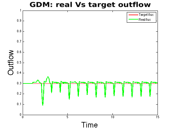
In Table 1, we see the different results obtained for the cost functional computed at the final time for the different policies. For comparison, we also put the results of the simulations with a constant speed equal to the minimum and maximal velocity bounds. The instantaneous policy is outperformed by the random exploration policy and by the gradient method. For the random exploration policy, in the table we put the minimal value of the cost functional computed by the algorithm. In Figure 7 we can see the distribution of the different values of the cost functional over 1000 simulations. Moreover, in Figure 8, we can see the differences between the actual outflow obtained and the target one for all methods.



We also compared the CPU time for the different simulations approaches (see Table 2). As expected, the random exploration policy is the least performing while the instantaneous policy is the fastest one.In addition, we computed the for each one of the policies obtaining the following results:
- •
IP:
- •
RE:
- •
GDM:
| Method | CPU Time (s) |
|---|---|
| Instantaneous policy | |
| Random exploration policy | |
| Gradient method |
4.3.2 Test II: Sinusoidal Outflow
In Figure 9, we show the optimal velocity obtained by using the instantaneous policy and by using the gradient descent method with a sinusoidal outflow. We show in Figure 10 the histogram of the cost functional obtained for the random exploration policy and in Figure 11 we compare the real outgoing flux with the target one.

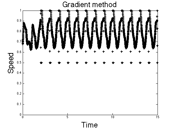


In Table 3, different results obtained for the cost functional computed at final time for the different policies are shown. Also in this case the instantaneous policy is outperformed by the other two. The CPU times give results similar to the previous test.
| Method | Cost Functional |
|---|---|
| Fixed speed | |
| Fixed speed | |
| Instantaneous policy | |
| Minimum of random exploration policy | |
| Gradient method |
5 Conclusions
In this work, we studied an optimal control problem for traffic regulation on a single road via variable speed limit. The traffic flow is described by the LWR model equipped with the Newell-Daganzo flux function. The optimal control problem consists in tracking a given target outflow in free flow conditions. We proved tje existence of a solution for the optimal control problem and provided explicit
analytical formulas for cost variations corresponding to
needle-like variations of the control policy.
We proposed three different control policies design: instantaneous depending
only on the instantaneous downstream density, random simulations and gradient descent.
The latter, based on numerical simulations for the cost variation, represents the best
compromise between performance, computational cost and total variation of the control policy.
Future works will include the study of this problem in case of congestion and the extension to second order traffic flow models.
Appendix
Lemma 3
Let , , , define and by . Using the change of variable we get:
| (22) |
Proof. The change of variable inside the integral gives
| (23) |
| (24) |
Observe that we need to specify the extremum in the integral, since the limit will provide Dirac terms inside the integral. We want now prove that the last addendum tends to zero. Denote by the distributional derivative of , which is a measure, and decompose it as in the continuous (AC+ Cantor) and Dirac part. By integrating , we write , with a continuous function, , and . Hence, by the mean value theorem applied to , we have
| (25) |
where is a point (depending on ) and the limit is zero as a consequence of the continuity of . The remaining term in (24) is then
Since is in the quantity tends to zero as tends to zero, thus we conclude.
Lemma 4
Proof.
We decompose the measure as ,
where is the Lebesgue measure, the Radon-Nikodym derivative of
w.r.t. , and . We approximate by piecewise
continuous functions defined as the integrals of , where is chosen such that .
Define and by its complement in .
Notice that for we have while on there are no jumps so
. We thus can write:
| (27) |
Since is in we can write:
Now, the following estimates hold:
We can write and , which gives us
where . Taking the limit for :
The last inequality holds true because
. Thus we get:
. Let us now estimate the quantity
Recalling that and we get
Passing to the limit in we conclude.
References
- [1] A. Alessandri, A. Di Febbraro, A. Ferrara, and E. Punta. Optimal control of freeways via speed signalling and ramp metering. Control Engineering Practice, 6:771–780, 1998.
- [2] A. Alessandri, A. Di Febbraro, A. Ferrara, and E. Punta. Nonlinear optimization for freeway control using variable-speed signaling. IEEE Transactions on vehicular technology, 48(6):2042–2052, 1999.
- [3] G. Allaire. Numerical analysis and optimization. Oxford university press, 2007.
- [4] Luigi Ambrosio, Nicola Fusco, and Diego Pallara. Functions of bounded variation and free discontinuity problems, volume 254. Clarendon Press Oxford, 2000.
- [5] M. K. Banda and M. Herty. Adjoint IMEX-based schemes for control problems governed by hyperbolic conservation laws. Computational optimization and applications, 51(2):909–930, 2010.
- [6] A. Bressan. Hyperbolic systems of conservation laws: the one-dimensional Cauchy problem. Oxford university press, 2000.
- [7] A. Bressan and B. Piccoli. Introduction to the mathematical theory of control. American Institute of Mathematical Sciences (AIMS), Springfield, MO, 2007.
- [8] G. Bretti, R. Natalini, and B. Piccoli. Fast algorithms for a traffic flow model on networks. Discrete and Continuous Dynamical Systems - Series B, 6(3):427–448, 2006.
- [9] C. Canudas De Wit. Best-effort highway traffic congestion control via variable speed limits. In 50th IEEE Conference on Decision and Control and European Control Conference, 2011.
- [10] R. C. Carlson, I. Papamichail, M. Papageorgiou, and A. Messmer. Optimal motorway traffic flow control involving variable speed limits and ramp metering. Transportation Science, 44:238–253, 2010.
- [11] R. M. Colombo and P. Goatin. A well posed conservation law with a variable unilateral constraint. J. Differential Equations, 234(2):654–675, 2007.
- [12] A. Csikós, I. Varga, and K. Hangos. Freeway shockwave control using ramp metering and variable speed limits. In 21st Mediterranean Conference on Control & Automation, pages 1569–1574, 2013.
- [13] C.F. Daganzo. The cell transmission model: A dynamic representation of highway traffic consistent with the hydrodynamic theory. Transportation Research Part B, 28:269–287, 1994.
- [14] J. R. Domíngeuz Frejo and E. F. Camacho. Global versus local MPC algorithms in freeway traffic control with ramp metering and variable speed limits. IEEE Transactions on intelligent transportation systems, 13(4):1556–1565, 2012.
- [15] C. Donadello and A. Marson. Stability of front tracking solutions to the initial and boundary value problem for systems of conservation laws. Nonlinear Differential Equations and Applications NoDEA, 14(5):569–592, 2007.
- [16] Lawrence C. Evans and Ronald F. Gariepy. Measure Theory and Fine Properties of Functions. CRC, 1991.
- [17] A. Fügenschuh, M. Herty, A. Klar, and A. Martin. Combinatorial and continuous model for the optimization of traffic flows on networks. SIAM Journal on optimization, 16(4):1155–1176, 2006.
- [18] M. Garavello and B. Piccoli. Traffic flow on networks, volume 1 of AIMS Series on Applied Mathematics. American Institute of Mathematical Sciences (AIMS), Springfield, MO, 2006. Conservation laws models.
- [19] M. Giles and S. Ulbrich. Convergence of linearized and adjoint approximations for discontinuous solutions of conservation laws. Part 2: Adjoint approximations and extensions. SIAM Journal on Numerical Analysis, 48(3):905–921, 2010.
- [20] P. Goatin, S. Göttlich, and O. Kolb. Speed limit and ramp meter control for traffic flow networks. Engineering Optimization, 2015, to appear.
- [21] S. K. Godunov. A finite difference method for the numerical computation of discontinuous solutions of the equations of fluid dynamics. Mathematicheckii Sbornik, 47:271–290, 1959.
- [22] M. Gugat, M. Herty, A. Klar, and Leugering. Optimal control for traffic flow networks. Journal of optimization theory and applications, 126(3):589–616, 2005.
- [23] A. Hegyi, B. De Schutter, and J. Hellendoorn. Model predictive control for optimal coordination of ramp metering and variable speed limits. Transportation Research Part C, 13(3):185–209, 2005.
- [24] A. Hegyi, B. De Schutter, and J. Hellendoorn. Optimal coordination of variable speed limit to suppress shock waves. IEEE Transactions on intelligent transportation systems, 6(1):102–112, 2005.
- [25] A. Hegyi and S. P. Hoogendoorn. Dynamic speed limit control to resolve shock waves on freeways - Field test results of the SPECIALIST algorithm. In 13th International IEEE Annual conference on Intelligent Transportation Systems, pages 519–524, 2010.
- [26] A. Hegyi, S. P. Hoogendoorn, M. Schreuder, and H. Stoelhorst. The expected effectivity of the dynamic speed limit algorithm SPECIALIST - a field data evaluation method. In Proceedings of the European Control Conference, pages 1770–1775, 2009.
- [27] A. Hegyi, S. P. Hoogendoorn, M. Schreuder, H. Stoelhorst, and F. Viti. SPECIALIST: A dynamic speed limit control algorithm based on shock wave theory. In Proceedings of the 11th International IEEE Conference on Intelligent Transportation Systems, pages 827 – 832, 2008.
- [28] Z. Hou, J.-X. Xu, and H. Zhong. Freeway traffic control using iterative learning control-based ramp metering and speed signaling. IEEE Transactions on vehicular technology, 56(2):466–477, 2007.
- [29] D. Jacquet, M. Krstic, and C. Canudas De Wit. Optimal control of scalar one-dimensional conservation laws. In Proceedings of the 2006 American Control Conference, pages 5213–5218, 2006.
- [30] S. N. Kružhkov. First order quasilinear equations with several independent variables. Mathematicheckii Sbornik, 81(123):228–255, 1970.
- [31] M. J. Lighthill and G. B. Whitham. On kinematic waves. II. A theory of traffic flow on long crowded roads. Proc. Roy. Soc. London Ser. A, 229:317–346, 1955.
- [32] J. Reilly, W. Krichene, M. L. Delle Monache, S. Samaranayake, P. Goatin, and A. M. Bayen. Adjoint-based optimization on a network of discretized scalar conservation law PDEs with applications to coordinated ramp metering. Journal of optimization theory and applications, 167(2):733–760, 2015.
- [33] P. I. Richards. Shock waves on the highway. Operations Research, 4:42–51, 1956.
- [34] S. Ulbrich. A sensitivity and adjoint calculus for discontinuous solutions of hyperbolic conservation laws with source terms. SIAM Journal on control and optimization, 41(3):740–797, 2002.
- [35] S. Ulbrich. Adjoint-based derivative computations for the optimal control of discontinuous solutions of hyperbolic conservations laws. Systems and control letters, 48(3):313–328, 2003.
- [36] X. Yang, Y. Lin, Y. Lu, and N. Zou. Optimal variable speed limit control for real-time freeway congestions. In Procedia Social and Behavioral Sciences, editors, 13th COTA International Conference of Transportation Professionals (CICTP 2013), volume 96, pages 2362–2372, 2013.