“K-theoretic” analog of Postnikov-Shapiro algebra distinguishes graphs
Abstract.
In this paper we study a filtered “-theoretical” analog of a graded algebra associated to any loopless graph which was introduced in [4]. We show that two such filtered algebras are isomorphic if and only if their graphs are isomorphic. We also study a large family of filtered generalizations of the latter graded algebra which includes the above “-theoretical” analog.
Key words and phrases:
spanning forests and trees, commutative algebras, filtered algebras2000 Mathematics Subject Classification
Primary 05E40, Secondary 05C311. Introduction
The following square-free algebra associated to an arbitrary vertex labeled graph was defined in [4], see also [1]. Let be a graph without loops on the vertex set (Below we always assume that all graphs might have multiple edges, but no loops). Throughout the whole paper, we fix a field of zero characteristic. Let be the graded commutative algebra over generated by the variables , with the defining relations:
Let be the subalgebra of generated by the elements
for where
| (1) |
For the reasons which will be clear soon, we call the spanning forests counting algebra of . Its Hilbert series and the set of defining relations were calculated in [5] following the initial paper [6]. Namely, let be the ideal in generated by the polynomials
| (2) |
where ranges over all nonempty subsets in and where is the total number of edges connecting a given vertex with all vertices outside . Thus, is the total number of edges between and the complementary set of vertices . Set
Remark 1.
Observe that since , we can define as the subalgebra of generated by .
We can also define as the quotient algebra of by the ideal generated by , where runs over all subsets of . This follows from the relation
To describe the Hilbert polynomial of we need the following classical notion going back to W. T. Tutte. Given a simple graph fix an arbitrary linear order of its edges. Now, given a spanning forest in (i.e., a subgraph without cycles which includes all vertices of ) and an edge in its complement, we say that is externally active for if there exists a cycle in such that all edges in belong to and is minimal in with respect to the chosen linear order. The total number of external edges is called the external activity of . Although the external activity of a given forest/tree in depends on the choice of a linear ordering of edges, the total number of forests/trees with a given external activity is independent of this ordering. Now we are ready to formulate the main result of [5].
Theorem 1.
[Theorems 3 and 4 of [5]] For any simple graph algebras and are isomorphic. The total dimension of these algebras (as vector spaces over ) is equal to the number of spanning subforests in . The dimension of the -th graded component of these algebras equals the number of subforests in with external activity . Here (resp. ) stands for the number of edges in (resp. ).
In the above notation, our main object will be the filtered subalgebra defined by the generators:
(Notice that we have one more generator here than in the previous case.)
Remark 2.
Since is obtained by exponentiation of we call the “K-theoretic” analog of .
Our first result is as follows. Define the ideal in as generated by the polynomials
| (3) |
where ranges over all nonempty subsets in and the number is the same as in (2). Set
Theorem 2.
For any graph algebras , and are isomorphic as (non-filtered) algebras.
Moreover, the following stronger statement holds.
Theorem 3.
For any graph , algebras and are isomorphic as filtered algebras.
Recall that in a recent paper [3] the first author has shown that contains all information about the matroid of and only it. Namely,
Theorem 4.
[Theorem 5 of [3]] Given two graphs and algebras and are isomorphic if and only if the matroids of and coincide. (The latter isomorphism can be thought of either as graded or as non-graded, the statement holds in both cases.)
On the other hand, filtered algebras and contain complete information about .
Theorem 5.
Given two graphs and without isolated vertices, and are isomorphic as filtered algebras if and only if and are isomorphic.
The structure of this paper is as follows. In § 2 we prove new results formulated above. In § 3 we discuss Hilbert series of similar algebras defined by other sets of generators. In § 4 we discuss “K-theoretic” analogs of algebras counting spanning trees. Finally, in § 5 we present a number of open problems.
Acknowledgements. The study of and was initiated by the second author jointly with Professor A. N. Kirillov during his visit to Stockholm in October-November 2009 supported by the Swedish Royal Academy. The second author is happy to acknowledge the importance of this visit for the present project and to dedicate this paper to Professor Kirillov.
2. Proofs
To prove Theorem 2, we need some preliminary results.
Lemma 1.
For any simple graph algebras and coincide as subalgebras of .
Proof.
Since where is the degree of vertex , then
Hence which means that .
To prove the opposite inclusion, consider . Since , we get
Using the relation , we conclude . Thus , implying that and coincide. ∎
Lemma 2.
For any simple graph algebras and are isomorphic as (non-filtered) algebras.
Proof.
First we change the variables in by using , . The generators of ideal transform as
for any subset .
Since for every vertex
we can consider as the quotient of the ring of formal power series factored by the ideal generated by all .
Similarly we can consider as the quotient of the ring of formal power series by the ideal generated by all .
Introduce the homomorphism defined by:
In fact, is an isomorphism, because is defined by .
Let us look at what happens with the ideal under the action of . For a given , consider the generator Then,
The factor is a formal power series starting with the constant term . Hence the last factor in the right-hand side of the latter expression is an invertible power series. Thus, the generator is mapped by to the product where is an invertible series. This implies . Hence algebras and are isomorphic. ∎
Proof of Theorem 2.
Proof of Theorem 3.
Consider the surjective homomorphism , defined by:
(It is indeed a homomorphism because every relation holds for .) By Theorem 2 we know that these algebras have the same dimension, implying that is an isomorphism. It is clear that preserves the filtration. ∎
2.1. Proving Theorem 5
We start with a few definitions.
Given a commutative algebra , its element is called reducible nilpotent if and only if there exists a presentation , where all are nilpotents.
For a nilpotent element , define its degree as the minimal non-negative integer for which there exists a reducible nilpotent element such that
Given an element , we say that an edge-element belongs to , if monomial has a non-zero coefficient in the expansion of as the sum of square-free monomials in .
Lemma 3.
For any nilpotent element , the degree of equals the number of edges of belonging to .
Proof.
We can write in terms of . (Observe that and coincide as subsets of , but have different graded/filtered structures). Now we can concentrate on the graded structure of . Select the part of which lies in the first graded component of . Thus
where is reducible nilpotent because it belongs to the linear span of other graded components. Thus . The statement of Lemma 3 is obvious for Additionally by construction, an edge-element belongs to if and only if it belongs to . ∎
Lemma 4.
Given a graph , let be the set of generators of corresponding to the vertices (i.e., ). Then
- (1)
are nilpotents;
- (2)
;
- (3)
for any subset and any set of pairwise distinct non-zero numbers (), the degree is equal to the number of edges incident to the vertices belonging to ;
- (4)
the number of edges between vertices and equals to .
Proof.
Item (1) is obvious.
To settle (2), observe that which implies
To prove (3), notice that, by Lemma 3, the degree is equal to the number of edges belonging to the sum . Each edge belongs either to zero, to one or to two generators from the latter sum. Moreover, if an edge belongs to two generators, then it has coefficients of opposite signs. Since all are different, an edge-element belongs to if and only if it belongs to at least one for . Thus the degree is the number of edges incident to all vertices from .
To settle (4), notice that if is an edge between vertices and , then belongs to and to with the opposite coefficients. Therefore does not belong to . Using Lemma 3, we get that equals twice the number of edges between and . ∎
Our proof of Theorem 5 uses the following technical lemma which should be obvious to the specialists.
Lemma 5 (Folklore).
Let be the set of edges of some graph without isolated vertices. If we know the following information:
- (1)
which pairs of edges are multiple, i.e., connect the same pair of vertices;
- (2)
which pairs of edges have exactly one common vertex;
- (3)
which triples of edges form a triangle,
then we can reconstruct up to an isomorphism.
Proof.
Assume the contrary, i.e., that there exist two non-isomorphic graphs and such that there exists a bijection of their edge sets and preserving (1) - (3). Assume that under this bijection an edge corresponds to the edge . Additionally assume that .
Now we construct an isomorphism between and . Let us split the vertices of into two subsets: where are all vertices which are incident to some pair of non-multiple edges.
Let us construct a bijection between the vertices of and , which extends the given bijection of edges, i.e., for any ,
At first we define it on . Namely, given a vertex choose two non-multiple edges and incident to it, and define as a common vertex of and We need to show that does not depend on the choice of and . It is enough to check it for a pair and , where is another edge incident to . Indeed, if has no common vertex with both and , then , and form a triangle in (because has a common vertex with and with ). Hence, , and form a triangle in , but they have a common vertex . Contradiction.
Now we need to extend to vertices belonging to . Note that each vertex has exactly one adjacent vertex. There are two possibilities.
Adjacent vertex of belongs to . Consider the edge (There might be several such edges, but this is not important, because in they are also multiple.) Knowing the image and the vertex , we define as the vertex of different from .
Adjacent vertex of belongs to . Consider edge Knowing , we define and as the vertices of edge (not important which is mapped to which).
Since has no isolated vertices and each edge has exactly two incident vertices from , we get that is surjective. Hence, is an isomorphism (otherwise it must be non-injective on vertices and, hence, ). Therefore and are isomorphic. ∎
Proof of Theorem 5.
Let and be a pair of graphs such that their filtered algebras and are isomorphic. Without loss of generality, we can assume that Denote the numbers of vertices in and by and resp.
We consider as a subalgebra in . The elements form a set of generators of . Denote by the elements corresponding to the vertices of under the isomorphism of filtered algebras. The set is also a generating set for which gives the same filtered structure and satisfies the assumptions of Lemma 4. In order to avoid confusion, we call the -th vertex of graph , and we call the -th vertex of graph .
Since and determine the same graded structure, then, in particular,
Additionally, by Lemma 4, and are nilpotents, implying that
Firstly, we need to show that each edge-element belongs to at most two different ’s. Assume the contrary, i.e., that belongs to and . Then there exist three distinct non-zero coefficients such that does not belong to . Moreover, for generic distinct non-zero coefficients , element () belongs to if and only if belongs to at least one of and . Hence by Lemma 3,
But at the same time, by Lemma 4 (3), they should coincide, contradiction.
By Lemma 4, for any , the degree equals to the valency of . Therefore,
because each edge-element is included in at most two . Since , we conclude that Furthermore, by Lemma 4 (2), each element belongs exactly to two vertices from with the opposite coefficients. Since we can additionally assume that the number of pairs of non-multiple edges which have a common vertex in is bigger than that in .
So far we have constructed a bijection between the edges of and the edges of . We want to prove that this bijection provides a graph isomorphism. We will achieve this as a result of the 5 claims collected in the following proposition which is closely related to Lemma 5.
Proposition 1.
The following facts hold.
- (1)
If and have no common vertex in , then they have no common vertex in as well.
- (2)
If and are multiple edges in , then they are multiple edges in as well.
- (3)
If and have exactly one common vertex in , then they have exactly one common vertex in as well.
- (4)
If , and form a star in , then they form a star in as well. (Three edges form a star if they have one common vertex and their three other ends are distinct.)
- (5)
If , and form a triangle in , then they form a triangle in as well.
Proof.
To prove (1), assume the contrary, i.e., assume that and belong to (and denote the corresponding coefficients by and resp.). Since elements have no monomial , then have no monomial as well (since their spans coincide). Then contains the monomial with the coefficient .
By Lemma 4 (2), we have , then there exists such that contains the monomial with a non-zero coefficient. Then must contain and (since does not contains ). Hence, has and with coefficients and resp. Therefore contains monomial with the coefficient . Thus the sum contains with coefficient , contradiction.
To prove (2), consider the map from to , sending an element from the span to the pair of coefficients of and resp. Since edges and are multiple in , the image of this map has dimension . If and are not multiple in , then the image of the map from has dimension .
To prove (3), observe that we have already settled Claims 1 and 2, and also we additionally assumed that the number of pairs of edges which have a common vertex in is bigger than that in . Then each such pair of edges from is mapped to the pair of edges from with the same property.
To prove (4), consider the map from to , sending an element in the span to the triple of coefficients of and resp. The image of this map has dimension . However if , and form a triangle in , then the image of the map from has dimension .
Proof of (5) is  similar to that of (4).∎
3. Further generalizations
In this section we will consider the Hilbert series of other filtered algebras similar to . (Recall that the Hilbert series of a filtered algebra is, by definition, the Hilbert series of its associated graded algebra.)
Let be a univariate polynomial or a formal power series over . We define the subalgebra as generated by together with
Example 1.
For , coincides with . For , coincides with .
Obviously, the filtered algebra does not depend on the constant term of From now on, we assume that has no constant term, since for any such that is constant, the filtered algebras and are the same.
Proposition 2.
Let be any polynomial with a non-vanishing linear term. Then algebras and coincide as subalgebras of .
Proof.
The argument is the same as in the proof of Lemma 1. We only need to change to and to . ∎
Theorem 6.
Let be any polynomial with non-vanishing linear and quadratic terms. Then given two simple graphs and and are isomorphic as filtered algebras if and only if and are isomorphic graphs.
Proof.
Repeat the proof of Theorem 5. ∎
3.1. Generic functions and their Hilbert series
Since for any , we can always truncate any polynomial (or a formal power series) at degree without changing . Therefore, for a given graph , it suffices to consider as a polynomial of degrees less than or equal to . To simplify our notation, let us write instead of .
Given a graph , consider the space of polynomials of degree less than or equal to and the corresponding Hilbert series.
Proposition 3.
In the above notation, for generic polynomials of degree at most , the Hilbert series is the same. This generic Hilbert series (denoted by below) is maximal in the majorization partial order among all where runs over the set of all formal power series with non-vanishing linear term.
Recall that, by definition, a sequence is bigger than in the majorization partial order if and only if, for any ,
More information about the majorization partial order can be found in e.g. [2].
Proof.
Note that, for a function the sum of the first entries of its Hilbert series equals the dimension of It is obvious that, for a generic this dimension is maximal. Since all Hilbert series are polynomials of degree at most then the required property has to be checked only for . Therefore it is obvious that, for generic , their Hilbert series is maximal in the majorization order. ∎
Remark 3.
ÃÂ We know that the Hilbert series of the graded algebra is a specialization of the Tutte polynomial of . However we can not calculate the Hilbert series of from the Tutte polynomial of , because there exists a pair of graphs with the same Tutte polynomial and different and , see Example 2.
Additionally, notice that, in general, . Analogously we can not calculate generic Hilbert series from the Tutte polynomial of , see Example 2.
Example 2.
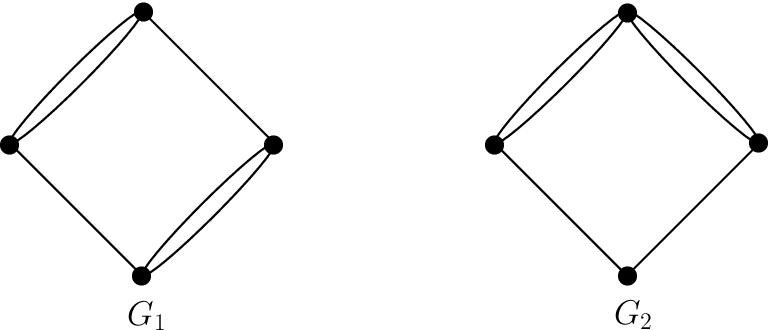
Consider two graphs and presented in Fig. 1. It is well-known that and have isomorphic matroids and hence, the same Tutte polynomial. Therefore, the Hilbert series of and coincide. Namely,
However, the Hilbert series of “K-theoretic” algebras are distinct. Namely
Moreover their generic Hilbert series are also distinct and different from their “K-theoretic” Hilbert series. Namely,
Putting our information together we get,
where denotes the majorization partial order.
4. “K-theoretical” analog for spanning trees
For an arbitrary loopless graph on the vertex set let be the graded commutative algebra over a given field generated by the variables , with the defining relations:
where a subgraph is called slim if its complement is connected.
Let be the subalgebra of generated by the elements
for where is given by (1). (Notice that and are defined by exactly the same formula but in different ambient algebras.)
Algebra will be called the spanning trees counting algebraÃÂ of and is, obviously, the quotient of modulo the set of relations over all non-slim subgraphs . Its defining set of relations is very natural and resembles that of (2). Namely, define the ideal in as generated by the polynomials:
| (4) |
where ranges over all nonempty subsets in and the number is the same as in (2). Set One of the results of [4] claims the following.
Theorem 7.
[Theorems 9.1 and Corollary 10.5 of [4]] For any simple graph on the set of vertices algebras and are isomorphic. Their total dimension is equal to the number of spanning trees in . The dimension of the -th graded component of equals the number of spanning trees in with external activity .
Similarly to the above, we can define the filtered algebra which is isomorphic to as a non-filtered algebra. Namely, is defined by the generators:
The first result of this section is as follows. Define the ideal as generated by the polynomials:
| (5) |
where ranges over all nonempty proper subsets in and the number is the same as in (2), together with the generator
| (6) |
Set
We present two results similar to the case of spanning forests.
Theorem 8.
For any simple graph algebras , and are isomorphic as (non-filtered) algebras. Their total dimension is equal to the number of spanning trees in .
Proof.
Theorem 9.
For any simple graph , algebras and are isomorphic as filtered algebras.
Proof.
Similar to the above proof of Theorem 3. ∎
To move further, we need to give a definition.
Definition 1.
Let be a connected graph. We define its -subgraph as the subgraph with following edges and vertices:
- •
if is not a bridge (i.e., is still connected),
- •
if there is an edge incident to .
In general, contains more information about than its matroid, because there exist graphs with isomorphic matroids and non-isomorphic -subgraphs, see Figure 2.
Recall that in a recent paper [3], the first author has shown that depends only on the bridge-free matroid of . Namely,
Proposition 4.
[Proposition 12 of [3]] For any two connected graphs and with isomorphic bridge-free matroids (matroids of their -subgraphs), algebras and are isomorphic.
Unfortunately, we can not prove the converse implication at present although we conjecture that is should hold as well, see Conjecture 6 in § 5. In case of filtered algebra and we can also prove an appropriate result only in one direction, see Proposition 5.
Similarly to § 3 we can to define . Let be a univariate polynomial or a formal power series over . We define the subalgebra as generated by and by
Proposition 5.
For univariate polynomial and any two connected graphs and with isomorphic -subgraphs and , algebras and are isomorphic as filtered algebras. Additionally, and are isomorphic as filtered algebras.
Proof.
Note that if has a bridge , then filtered algebra is the Cartesian product of filtered algebras and , where and are connected component of .
Thus filtered algebra is the Cartesian product of such filtered algebras corresponding to the connected components of the -subgraph of .
Therefore if connected graphs and have isomorphic -subgraphs, then their filtered algebras and are isomorphic. ∎
Remark 4.
In general case we can not prove that these algebras distinguish graphs with different -subgraphs. The proof of Theorem 5 does not work for two reasons. Firstly, is not the degree of the -th vertex in . Secondly, even if we can construct a similar bijection between edges, we do not have an analog of Proposition 1. Since in the proof we consider coefficients of monomial , in case when and are not bridges and when is a cut, this monomial can still lie in the ideal.
It is possible to construct such a bijection in a smaller set of graphs, namely for graphs such that, for any edge in the graph, there is another edge which is multiple to . For such graphs we do not have the second problem, because if is a cut, then and are multiple edges. So, instead of the actual converse of Proposition 5, we can prove the converse in the latter situation, but we do not present this result here.
Proposition 6.
In the above notation, for generic polynomials of degree at most , the Hilbert series is the same. This generic Hilbert series (denoted by below) is maximal in the majorization partial order among for running over the set of power series with non-vanishing linear term.
Proof.
See the proof of Proposition 3. ∎
Example 3.
Consider two graphs and , see Fig. 2. It is easy to check that subgraphs and have isomorphic matroids, implying that algebras and are isomorphic.

The Hilbert series of “K-theoretic” algebras are distinct, namely
These graphs are “small”, so their generic Hilbert series coincides with the “K-theoretic” one. Putting our information together, we get
5. Related problems.
At first, we formulate several problems in case of spanning forests; their analogs for spanning trees are straight-forward.
Problem 1.
For which functions besides and , one can present relations in for any graph in a simple way? In other words, for which one can define an algebra similar to and ?
Since the Hilbert series and are not expressible in terms of the Tutte polynomial of , they contain some other information about .
Problem 2.
Find combinatorial description of and ?
Problem 3.
For which graphs , Hilbert series and coincide? In other words, for which , is a generic function?
Problem 4.
Describe combinatorial properties of when is a function starting with a monomial of degree bigger than , i.e. ? In particular, calculate the total dimension of .
The most delicate and intriguing question is as follows.
Problem 5.
Do there exist non-isomorphic graphs and such that, for any polynomial , the Hilbert series and coincide? In other words, does the collection of Hilbert series taken over all formal series determine up to isomorphism?
The following problems deal with the case of spanning trees only.
Conjecture 6.
[comp. [3]] Algebras and for graphs and are isomorphic if and only if their bridge-free matroids are isomorphic, where the bridge-free matroid is the graphical matroid of -subgraph.
Problem 7.
Which class of graphs satisfies the property that if two graphs and from this class have isomorphic and , then their -subgraphs are isomorphic. In other words, can one classify all pairs of connected graphs, which has isomorphic filtered algebras and ? (The same problem for and , where )
References
- [1] F. Ardila, A. Postnikov, Combinatorics and geometry of power ideals, Trans. of the AMS, 362(8), (2010), 4357–4384.
- [2] A. W. Marshall, I. Olkin, B. Arnold, Inequalities: Theory of Majorization and Its Applications, Second edition. Springer Series in Statistics. Springer, New York, 2011.
- [3] G. Nenashev, On Postnikov-Shapiro Algebras and their generalizations, arXiv:1509.08736.
- [4] A. Postnikov, B. Shapiro, Trees, parking functions, syzygies, and deformations of monomial ideals. Trans. Amer. Math. Soc. 356(8) (2004), 3109–3142
- [5] ÃÂA. Postnikov, B. Shapiro, M. Shapiro, Algebras of curvature forms on homogeneous manifolds. Differential topology, infinite-dimensional Lie algebras, and applications, 227–235, Amer. Math. Soc. Transl. Ser. 2, 194, Amer. Math. Soc., Providence, RI, 1999
- [6] ÃÂB. Shapiro, M. Shapiro, On ring generated by Chern -forms on . C. R. Acad. Sci. Paris SÃÂÃÂÃÂÃÂÃÂÃÂÃÂÃÂÃÂÃÂÃÂÃÂÃÂÃÂÃÂÃÂr. I Math. 326(1) (1998), 75–80.