Fracton Topological Order, Generalized Lattice Gauge Theory and Duality
Abstract
We introduce a generalization of conventional lattice gauge theory to describe fracton topological phases, which are characterized by immobile, point-like topological excitations, and sub-extensive topological degeneracy. We demonstrate a duality between fracton topological order and interacting spin systems with symmetries along extensive, lower-dimensional subsystems, which may be used to systematically search for and characterize fracton topological phases. Commutative algebra and elementary algebraic geometry provide an effective mathematical toolset for our results. Our work paves the way for identifying possible material realizations of fracton topological phases.
Topological phases of matter are currently attracting tremendous interest from diverse disciplines such as theoretical physics, quantum information and quantum materials. Gauge theory provides a unified framework for understanding several important topological phases, from quantum Hall states to quantum spin liquids [1, 2, 3, 4, 6, 5, 7, 8, 9, 10, 11]. The fractional statistics of topological excitations [12, 13], or anyons, can be understood from the Aharanov-Bohm phase of a charge moving around a flux. The topological degeneracy of the ground state is characterized by the holonomy of a locally flat gauge connection around non-contractible loops.
Recently, a new kind of topological phase which does not fit into the framework of gauge theory has been discovered in exactly solvable lattice models in three dimensions [16, 14, 15, 17, 18]. A remarkable property of this new phase is the existence of point-like fractional excitations termed “fractons” [18], which can only be created at the corners of membrane- or fractal-like operators, unlike anyons that are created at the ends of Wilson lines. The creation of anyons at the two ends of a Wilson line immediately implies that anyons can move by repeated application of a local, line-like operator. In contrast, the absence of any operator that can create a pair of fractons implies that a single fracton cannot move without creating additional excitations, i.e. fractons are fundamentally immobile. Thus far, two broad classes of fracton topological orders have been found:
- Type I
- Type II
Fracton topological order provides an exciting development in the search for new quantum phases of matter, for new schemes for quantum information processing [21], and in the investigation of glassy dynamics in interacting quantum systems [20]. Fractons enable new forms of electron fractionalization [18], and provide an alternative to Fermi or Bose statistics in three dimensions. Fractons may be used to build a robust, finite-temperature quantum memory, as theoretically demonstrated for Haah’s code [16, 19]. The innately slow dynamics of fractons provides an intriguing connection with quantum glasses, many-body localization, and a new testing ground for the postulates of quantum statistical mechanics.
Research on fracton topological phases is in its early stages and has been based on studies of specific lattice models. It is thus highly desirable to find a more unified theoretical framework for fracton topological order. In this work, we demonstrate that fracton topological phases can be obtained as the quantum dual of -dimensional systems that possess “subsystem symmetries”, namely a set of symmetries associated with subsystems of dimension . Specifically, we establish an exact duality relating both type-I and type-II fracton topological orders to symmetry-breaking order in quantum systems with subsystem symmetries along planes and fractals, respectively. This duality between fracton topological order and subsystem symmetry-breaking, hereafter referred to as the “F-S” duality, is naturally obtained from a generalized lattice gauge theory which we introduce. Instead of placing a gauge field on links between neighboring sites as in a standard lattice gauge theory, we introduce a new field to mediate multi-body interactions between matter fields on a cluster of neighboring sites. This yields an interacting quantum system with a generalized Gauss’ law that characterizes the fracton topological phase.
Before describing our construction in generality, we present a concrete example that yields a new class of type-I fracton topological phases. Consider a model of Ising spins at the sites of a three-dimensional cubic lattice, whose Hamiltonian () is defined to be a sum of four-spin interactions at each plaquette, as shown in Table 1. This classical “plaquette Ising model” is invariant under a spin-flip along any , or -plane of the cubic lattice. The plaquette Ising model has a rich history of study, attracting interest as a model for the statistical mechanics of smooth surfaces, and as a lattice regularization of string theory [27, 28, 29, 30, 31, 32].
We introduce a generalized lattice gauge theory to construct the quantum dual of the plaquette Ising model in a transverse field. This generalizes Wegner’s duality [1] between the -dimensional transverse-field Ising model and Ising lattice gauge theory [2]. Wegner’s duality is motivated by the observation that a configuration of Ising spins may be specified by the locations of the domain walls between symmetry-breaking states of the Ising model. As a result, a dual representation of the Ising matter is given by Ising “domain wall” fields on the links of the lattice. Furthermore, since domain walls form closed, ()-dimensional surfaces, physical states in the domain wall Hilbert space must satisfy a local “zero-flux” condition, that the lattice curl of the domain wall spins vanishes around each plaquette. In this way, the -dimensional transverse-field Ising model is dual to lattice gauge theory.
Our duality between fracton topological order and subsystem symmetry-breaking is obtained by a similar observation. A configuration of Ising spins may, equivalently, be specified by the eigenvalue of each interaction term in the Hamiltonian [33]. For example, to obtain the dual of the plaquette Ising model, we are naturally led to introduce the Ising fields at the center of each plaquette. Physically, the field labels the presence or absence of a domain wall between the subsystem symmetry-breaking ground-states of the plaquette Ising Hamiltonian. While domain walls in the ordinary Ising model form closed surfaces, the fields in our model must satisfy more exotic local constraints due to the geometry of the plaquette interactions to ensure a one-to-one correspondence with the physical space of domain walls in .
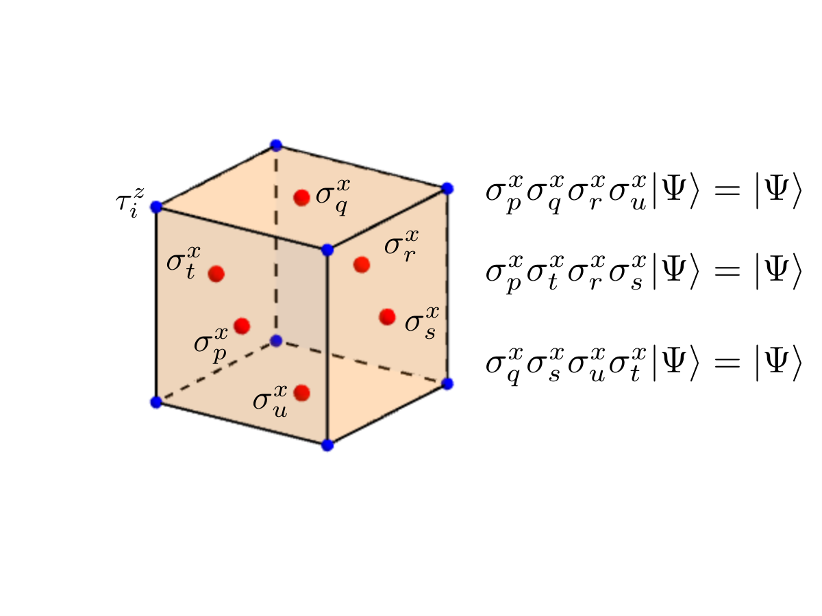
As we demonstrate below, the quantum dual of the plaquette Ising Hamiltonian, in terms of the fields, exhibits fracton topological order. The resulting fracton Hamiltonian has a solvable limit, analogous to the deconfined phase of a conventional gauge theory, which is given by a Hamiltonian for the Ising fields (), now placed at the links of the dual cubic lattice. As shown in Table 1, this fracton Hamiltonian consists of two types of terms: (1) a twelve-spin interaction for the spins surrounding a dual cube and (2) four-spin -interactions at each vertex of the dual cubic lattice that are aligned along the , and -planes. The cubic and cross-like geometries of the interactions motivate the name “X-cube” model. The ground-state is topologically-ordered, as the ground-states are locally indistinguishable, and one of the fundamental excitations – obtained by flipping the eigenvalue of the cubic interaction term – is a fracton. This can be seen by observing that there is no local operator that can create a single pair of cube excitations. For example, the operator creates four cube excitations when acting on the ground-state. Repeated application of over a membrane separates the four cube excitations to each corner as shown in Figure 1a. Therefore, a single cube excitation is fundamentally immobile, and cannot move without creating additional cube excitations. Pairs of cube excitations, however, can be moved by sequentially applying a local, membrane-like operator.
The quasiparticle content of the X-cube model is summarized in Table 1, along with other fracton phases such as Haah’s code, the CBLT model, and a new spin model which we introduce and term the “checkerboard model”. All of these phases are obtained by applying our generalized lattice gauge theory prescription to spin models with subsystem symmetries. As we will demonstrate, a simple property of the classical spin model, that no product of interaction terms acts exclusively on a pair of isolated spins, guarantees that its quantum dual exhibits fracton topological order.
More generally, consider a classical Hamiltonian for Ising spins at the sites of a three-dimensional Bravais lattice. We assume, for simplicity of presentation, that there is a single spin at each lattice site; the case where the unit cell is larger is explained in the Appendix. The Hamiltonian consists of types of interactions at each lattice site , and may be written in the form:
| (1) |
with the constant . We demonstrate that a classical spin Hamiltonian (1) satisfying certain simple properties may be used to build a topologically-ordered, quantum system with fracton excitations. First, we require that the spin Hamiltonian (1) has a subsystem symmetry under which the spin-flip transformation along non-local subsystems of the lattice – i.e. subsystems that scale with the system size – leaves invariant. We further require that has no local symmetries. In this sense, a subsystem symmetry is “intermediate” between local and global symmetries [22, 23]. For the remainder of this work, we will refer to the plaquette Ising model () and the tetrahedral Ising Hamiltonian as concrete examples. As shown in Table 1, the Hamiltonian is defined on the face- centered cubic (fcc) lattice and consists of nearest-neighbor four-spin interactions that form elementary tetrahedra. The tetrahedral Ising model has two interaction terms per site on the fcc lattice. Both the tetrahedral and plaquette Ising models have a subsystem symmetry, as they are invariant under spin-flips along orthogonal planes (, or ).
An important consequence of the subsystem symmetry of the spin Hamiltonian is that the resulting ground-state has sub-extensive classical degeneracy , taking the form on the length- three-torus. Since the degeneracy is classical in nature, each ground-state may be distinguished by a local order parameter. Transitioning between ground-states, however, requires performing a spin-flip along a subsystem. While a local perturbation can lift the classical degeneracy, no local operator can connect distinct ground-states.
I Generalized Lattice Gauge Theory and the F-S Duality
We now build a quantum Hamiltonian with fracton topological order by promoting the subsystem symmetry of the spin system (1) to a local symmetry. We begin by adding a transverse field at each lattice site to allow the classical spins to exhibit quantum fluctuations. Next, we introduce additional Ising spins at the center of each multi-spin interaction appearing in ; these spins appear at the sites of a lattice with an -site basis. We introduce a minimal coupling between the spins and the Ising matter fields, by coupling each to its corresponding multi-spin interaction:
| (2) |
After this minimal coupling, the Hamiltonian describing both and Ising matter fields is given by
| (3) |
We refer to as the nexus field, as each is placed at the center of an elementary multi-spin interaction of the classical spin Hamiltonian. We will soon observe that the nexus field provides a natural generalization of a gauge field in a conventional lattice gauge theory. In contrast to our construction, applying the standard gauging procedure to any of the spin models shown in Table 1 by introducing a gauge field on the links of the cubic lattice would result in a Hamiltonian with conventional topological order. Our procedure is also distinct from discretizations of “higher-form” gauge theories, in which interactions between -form matter fields are mediated by an -form gauge field [34, 35].
The subsystem symmetry of the classical spin system (1) has now been promoted to a local spin- flip symmetry of the Hamiltonian (3). While – the generator of a single spin-flip – anti-commutes with several multi-spin interactions in (1), this can be compensated by acting with the nexus field on the lattice sites associated with these interactions. As a result, the operator
| (4) |
where
| (5) |
generates a local symmetry of the Hamiltonian (). The set specifies the locations of multi-spin interactions that anti-commute with .
We proceed to add all other interaction terms involving the nexus field and the Ising spins that are consistent with this local spin-flip symmetry. To lowest-order, we include a transverse field for the matter and nexus fields:
| (6) |
Since the operator generates a local symmetry of the Hamiltonian, we may impose the condition on the Hilbert space, which amounts to a generalized Gauss’s law. In analogy with conventional gauge theory, we will refer to as the nexus charge operator. As an example, the nexus charge operator in the X-code model is given by the product of on twelve spins sitting at the links surrounding a cube, as shown in Table 1.
Since the generalized Gauss’s law condition commutes with the spin-nexus Hamiltonian (6), it is possible to choose a “gauge” that completely eliminates the Ising matter fields, and yields a Hamiltonian exclusively for the nexus spins. First, we impose the generalized Gauss’s law to obtain a Hamiltonian acting within the constrained Hilbert space
| (7) |
Since each operator commutes with the Hamiltonian, we may restrict our attention to states in the constrained Hilbert space that satisfy . This yields the gauge-fixed Hamiltonian
| (8) |
When , it is convenient to identify an effective Hamiltonian that takes the form
| (9) |
where we have introduced operators at each lattice site . These operators are determined in perturbation theory by computing the simplest product of terms near a given lattice site that commute with the nexus charge . As an example the operators obtained by applying this construction to the plaquette Ising model are shown in Table 1.
Our proposal bears resemblance to the construction of a conventional lattice gauge theory. First, the Hamiltonian for gauge theory is recovered from the general form of the Hamiltonian for the Ising matter and nexus fields (6) if the matter fields couple through nearest-neighbor two-body interactions, so that where is nearest-neighbor to site . This is in contrast to the multi-body interactions that are present in our models with subsystem symmetry. In the gauge-fixed Hamiltonian (8), then becomes the familiar charge operator, while the operator , appearing in the effective Hamiltonian , precisely measures the flux through an elementary plaquette.
| Explanation | ||
| A classical configuration of Ising spins () may be specified by spins () placed at the centers of each of the interaction terms for the Ising matter. | ||
| The dual representation of is given by the nexus charge , defined as the product of terms that correspond to the interactions flipped by . | ||
| A local product of interactions for the Ising matter fields that yields the identity corresponds to a constraint on the dual Hilbert space. The constraint restricts the Hilbert space of to that of domain wall configurations in the ordered phase of . | ||
| A product of operators is dual to a product of interaction terms for the matter fields. As a result, the nexus charge is a fracton only if there is no product of interaction terms that can create an isolated pair of spin-flips. |
Within our construction, the operators provide the natural generalization of the flux in a lattice gauge theory. As the excitation obtained by flipping the eigenvalue of a operator is often point-like, we will refer to the excitation as a “generalized monopole”. While the flux is always a line-like excitation in a three-dimensional Abelian lattice gauge theory, the behavior of the “generalized monopole” can be quite varied. As an example, the generalized monopole is a fracton in both the checkerboard spin model and in Haah’s code, but is free to move along a line without creating additional excitations in the X-cube model. We refer to such an excitation as a dimension-1 quasiparticle [18], as the excitation is only mobile along a line. As shown in Figure 1b, a straight Wilson line can create an isolated pair of the generalized monopole excitations in the X-cube model, which can only move along the line without creating additional excitations. Within type-I fracton topological order, composites of the fracton charge excitations that are mobile in two dimensions can have non-trivial mutual statistics with the generalized monopole. This is true in both the checkerboard and X-cube models, where an anyon formed from a composite of two fracton charges has -statistics with a generalized monopole in its plane of motion.

We now consider the generalized lattice gauge theory (8) when , so that the nexus field (defined in the -basis) has no dynamics. The resulting Hamiltonian
| (10) |
has a local symmetry, as the operators commute with each term in (10). We refer to the emergent local constraints on the Hilbert space
| (11) |
as the generalized “flatness” condition, analogous to a flat connection in a continuum gauge theory, as these constraints are obtained in the limit that there is zero “flux” of the nexus field.
Our construction of a generalized lattice gauge theory implies that the quantum dual of the Ising matter in the presence of a transverse field:
| (12) |
is precisely given by the nexus Hamiltonian (10), combined with the generalized flatness condition (11).
Without appealing to the generalized lattice gauge theory, the duality can be obtained directly from the Hamiltonian . A dual representation is constructed by placing the nexus spins at the centers of the interactions . The nexus spins are now interpreted as domain wall variables for the ordered phase () of the spin model . The nexus spins must satisfy local constraints due to the geometry of the multi-spin interactions in order to correspond to the physical space of domain walls between ground-states of . These local constraints are precisely given by the generalized flatness condition (11). As an example, the generalized monopole operators for the plaquette Ising model are obtained by noting that the product of four plaquette interactions that wrap a cube is equal to the identity. Our F-S duality implies a map between local operators in the Hilbert spaces of the Ising matter and nexus fields, as summarized in Table 2. As an example, a domain wall in the ground-state of the plaquette Ising model is shown in Figure 2.
II Fracton Topological Order
We now invoke the F-S duality to demonstrate that the commuting Hamiltonian
| (13) |
exhibits fracton topological order. We argue that (i) the spectrum of has sub-extensive topological degeneracy and that (ii) the nexus charge is fundamentally immobile. We provide rigorous proofs of these statements in the Appendix using techniques in commutative algebra and elementary algebraic geometry, which provide effective mathematical tools to study the subsystem symmetries of classical spin models, as well as the ground-state degeneracy and excitation spectrum of fracton topological phases. An algebraic representation of a classical Ising system defines an algebraic variety over the field of characteristic 2 (), defined by addition and multiplication [25]. Two conditions on this variety, as derived in the Appendix from the Buchsbaum-Eisenbud criterion [36, 37] for the exactness of a complex of free modules, guarantee that the quantum dual exhibits fracton topological order.
We begin by using the F-S duality to demonstrate that the sub-extensive degeneracy of the classical, ground-state of implies that the Hamiltonian has sub-extensive topological ground-state degeneracy on the torus. Recall that a product of operators along an appropriate subsystem generates a symmetry of the Hamiltonian . When , the ground-state exhibits classical, sub-extensive degeneracy since there are independent subsystems along which a spin-flip commutes with all of the interaction terms . The plaquette Ising model, for example, commutes with the product of along a plane, and the ground-state has sub-extensive, classical degeneracy since there are independent planes along which a spin-flip may be performed.
From the operator dictionary for the F-S duality, the dual representation of this spin-flip operator is given by a product of nexus charges along the same subsystem . Furthermore, each interaction term is dual to a single-spin operator . Since the F-S duality preserves the commutation relations between operators, we conclude that due to the subsystem symmetry of , the operators in the dual theory satisfy:
| (14) |
for all , . This commutation relation can only be satisfied if the product of nexus charges along yields the identity, so that . This relation implies that not all of the nexus charge operators are independent on the torus. Each of the independent subsystems associated with the subsystem symmetry of reduces the number of independent nexus charge operators by one. We denote the total number of such independent subsystems by .
In the ground-state of the fracton Hamiltonian, the -dimensional Hilbert space of nexus spins is constrained by the nexus charge and monopole operators that appear in the Hamiltonian. However, only of the operators are independent on the torus, where is the number of “dependency relations” on both the nexus charge and monopole operators. The topological ground-state degeneracy on the torus is given by . When the number of interactions appearing in is identical to the total number of nexus spins (), as is the case for all of the fracton models considered in this work, the topological degeneracy is precisely . In this case, the sub-extensive degeneracy of the ground-state of the spin model provides a lower bound on the topological degeneracy of . For example, the checkerboard spin model has topological ground-state degeneracy on the length- three-torus, as we compute in the Appendix, while the tetrahedral Ising model only has classical degeneracy since the model has subystem symmetries along three orthogonal planes.
In addition to the sub-extensive, topological degeneracy of , we also wish to show that that there is no degeneracy in the spectrum of Hamiltonian due to the presence of local observables. In the absence of local observables, the local reduced density matrix will be identical for any degenerate states in the spectrum of the Hamiltonian, and the topological degeneracy, as computed by constraint-counting, will be stable to local perturbations [26]. As we demonstrate in the Appendix, the ground-states of are guaranteed to be locally indistinguishable, provided that the classical spin system has no lower-dimensional symmetries along subsystems of dimension (e.g. line-like symmetries). We prove this by using an algebraic representation of and also argue this as a consequence of the F-S duality.
Having demonstrated that exhibits sub-extensive topological degeneracy and that the degenerate ground-states are locally indistinguishable, we now demonstrate that the nexus charge is indeed a fracton excitation, provided that the spin model (12) satisfies a simple condition. Consider acting on the ground-state of with the operator
| (15) |
where is some subset of the lattice. The operator will create nexus charge excitations by anti-commuting with a collection of operators. Invoking the F-S duality, we observe that the pattern of excitations created by is precisely given by the location of spin-flips created by the dual operator when acting on the paramagnetic state . The spectrum of contains fractons only if there is no operator of the form that can create a single pair of spin-flip excitations. If such an operator did exist, then it would be possible to move a single nexus charge without any energy cost and the charge would be mobile.
Our condition for the existence of fracton excitations is simple to demonstrate for the plaquette Ising and tetrahedral Ising Hamiltonians. Here, it is evident that any product of the four-spin interactions shown in Table 1 creates at least four spin-flip excitations when acting on the paramagnetic state . Therefore, the nexus charge for each of the corresponding Hamiltonians is a fracton. In fact, if any Ising Hamiltonian has a subsystem symmetry along three orthogonal planes, and two or more independent interactions per lattice site, then the quantum dual will always exhibit fracton topological order, as we demonstrate in the Appendix. All Type-I fracton topological phases that have been discovered thus far fit into this framework.
We now summarize the precise conditions on the classical spin system , as derived in the Appendix using the algebraic representation of the classical spin system, that guarantee that exhibits fracton topological order:
- 1.
contains more than one independent interaction term per lattice site
- 2.
No product of the interaction terms () can generate an isolated pair of spin-flips
III Phase Diagram
We discuss the phase diagram of the spin-nexus Hamiltonian (6). In the limit , the nexus field decouples from the Ising matter; is set to 1, and the effective Hamiltonian for the nexus field is
| (16) |
The generalized Gauss’ law becomes . Here, is some power of as is obtained from perturbation theory. When , the nexus field forms a fracton phase that is described by Hamiltonian . The topologically-ordered fracton phase and the Ising paramagnet survive up to a finite and , as both phases are gapped and stable to perturbations [26].
Confinement: From the topologically-ordered fracton phase, we may proceed in two directions. First, we consider increasing while keeping , a constant. Above a critical value , the ground-state will be a condensate of nexus flux excitations and the fracton topological order will be destroyed. The nature of the transition between the fracton phase and the trivial (confined) phase is currently unknown.
‘Higgs’ Phase: We now consider the region of the phase diagram where , keeping at a fixed constant. Here, the matter fields enter an ordered state with . This may be seen as the analog of a ‘Higgs’ phase, as the Ising order gives the nexus field a mass that destroys the fracton topological phase. The ground-state in this region of the phase diagram is non-degenerate, even though the ordered phase of the pure spin model (12) has sub-extensive degeneracy. We may demonstrate this by observing that in the gauge-fixed Hamiltonian (8), increasing destroys the fracton topological order by condensing the nexus charge, and produces a non-degenerate ground-state. We also observe from that the confined and Higgs regions of the spin-nexus phase diagram are smoothly connected, as in the Ising lattice gauge theory. We summarize our schematic phase diagram in Fig. 4a.
In passing, we observe that the checkerboard fracton Hamiltonian in Table 1 in the presence of two transverse fields has a symmetry under . This implies that the phase diagram should be symmetric under and . The confinement and ‘Higgs’ transition must be dual to each other, and the line of phase transitions must meet at a self-dual point of the phase diagram. It is unknown whether any of the indicated phase transitions in Fig. 4 are continuous.
IV Concluding remarks
Translationally-invariant, commuting Hamiltonians built from interacting qubits [25] and fermions [18] admit a convenient algebraic representation as a collection of polynomials over a finite field. The translation group of the lattice is , whose group algebra happens to be the polynomial algebra. The polynomials conveniently keep track of the support of various operators. Remarkably, this algebraic characterization of the Hamiltonian terms enable us to decide whether the given Hamiltonians is commuting, degenerate, topologically ordered, and the nature of the excitations [18, 25]. Also, it gives a unique method to calculate the ground-state degeneracy of our exotic models. In the context of our nexus theory, the polynomial representation has a natural physical interpretation, as it precisely specifies the generalized Gauss’ law that defines the spin-nexus Hamiltonian (6). In this way, the polynomial representation encodes the local symmetry that defines a fracton topological phase. We elaborate on these method in the appendix, which we aim to be pedagogical.
With the identification of a generalized Gauss’s law that characterizes a fracton topological phase, our work provides an important step towards searching for material realizations of fracton topological order. Such a local conservation law can, in principle, appear in physical systems such as frustrated magnets, where our generalized gauge theory can emerge as an effective description at low energies, leading to fracton topological order.
Note Added: Near the completion of this work, we were informed that a related work is being written up [38].
Acknowledgements.
This work was supported by the David and Lucile Packard Foundation (LF and SV) and the Pappalardo Fellowship in Physics at MIT (JH).References
- [1] F. Wegner, “Duality in Generalized Ising Models and Phase Transitions without Local Order Parameters”, J. Math Phys. 12, 2259 (1971).
- [2] E. Fradkin and S. Shenker, “Phase diagrams of lattice gauge theories with Higgs fields”, Phys. Rev. D 19, 3682 (1979).
- [3] S. C. Zhang, T. H. Hansson, and S. Kivelson, “Effective-Field-Theory Model for the Fractional Quantum Hall Effect”, Phys. Rev. Lett. 62, 82 (1989).
- [4] X. G. Wen and Q. Niu, “Ground-state degeneracy of the fractional quantum Hall states in the presence of a random potential and on high-genus Riemann surfaces”, Phys. Rev. B 41, 9377 (1990).
- [5] S. Sachdev and N. Read, “Large- expansion for frustrated quantum antiferromagnets”, Phys. Rev. Lett. 66, 1773 (1991).
- [6] X. G. Wen, “Mean-field theory of spin-liquid states with finite energy gap and topological orders”, Phys. Rev. B 44, 2664 (1991).
- [7] T. Senthil and M. P. A. Fisher, “ gauge theory of electron fractionalization in strongly correlated systems”, Phys. Rev. B 62, 7850 (2000).
- [8] R. Moessner, S. L. Sondhi, “Resonating Valence Bond Phase in the Triangular Lattice Quantum Dimer Model”, Phys. Rev. Lett 86, 1881 (2001).
- [9] A. Yu. Kitaev, “Fault-tolerant quantum computation by anyons”, Annals Phys. 303, 2 (2003).
- [10] M. Hermele, M. P. A. Fisher, L. Balents, “Pyrochlore photons: The spin liquid in a three-dimensional frustrated magnet”, Phys. Rev. B 69, 064404 (2004).
- [11] X. G. Wen, Quantum Field Theory of Many-Body Systems. Oxford University Press, Oxford (2004).
- [12] B. I. Halperin, “Statistics of Quasiparticles and the Hierarchy of Fractional Quantized Hall States”, Phys. Rev. Lett. 52, 1583 (1984).
- [13] D. Arovas, J. R. Schrieffer, and F. Wilczek, “Fractional Statistics and the Quantum Hall Effect”, Phys. Rev. Lett. 53, 722 (1984).
- [14] C. Chamon, “Quantum Glassiness in Strongly Correlated Clean Systems: An Example of Topological Overprotection”, Phys. Rev. Lett. 94, 040402 (2005).
- [15] S. Bravyi, B. Leemhuis, and B. Terhal, “Topological order in an exactly solvable 3D spin model”, Ann. Phys. 326, 839 (2011).
- [16] J. Haah, “Local stabilizer codes in three dimensions without string logical operators”, Phys. Rev. A 83, 042330 (2011).
- [17] B. Yoshida, “Exotic topological order in fractal spin liquids”, Phys. Rev. B 88, 125122 (2013).
- [18] S. Vijay, J. Haah and L. Fu, “A New Kind of Topological Quantum Order: A Dimensional Hierarchy of Quasiparticles Built from Stationary Excitations”, Phys. Rev. B 92, 235136 (2015).
- [19] S. Bravyi and J. Haah, “Quantum Self-Correction in the 3D Cubic Code Model”, Phys. Rev. Lett. 111, 200501 (2013).
- [20] I. H. Kim and J. Haah, “Localization from Superselection Rules in Translationally Invariant Systems”, Phys. Rev. Lett. 116, 027202 (2016).
- [21] B. M. Terhal, “Quantum error correction for quantum memories”, Rev. Mod. Phys. 87, 307 (2015).
- [22] C. D. Batista and Zohar Nussinov, Phys. Rev. B 72, 045137 (2005).
- [23] Z. Nussinov and E. Fradkin, “Discrete Sliding Symmetries, Dualities, and Self-dualities of Quantum Orbital Compass Models and Superconducting Arrays”, Phys. Rev. B 71, 195120 (2005).
- [24] N. Read, “Topological phases and quasiparticle braiding”, Physics Today, 65, 38 (2012);
- [25] J. Haah, “Commuting Pauli Hamiltonians as maps between free modules”, Commun. Math. Phys. 324 351-399 (2013)..
- [26] S. Bravyi, M. Hastings and S. Michalakis, “Topological quantum order: stability under local perturbations”, J. Math. Phys. 51 093512 (2010).
- [27] G. K. Savvidy and F. J. Wegner, “Geometrical string and spin systems ”, Nucl. Phys. B 413, 605 (1994).
- [28] G. K. Savvidy and K. G. Savvidy, “Self-avoiding surfaces and spin systems”, Physics Letters B 324 72-77 (1994).
- [29] G. K. Savvidy and K. G. Savvidy, “Interaction hierarchy: string and quantum gravity”, Modern Physics Letters A 11 1379-1396 (1996).
- [30] R. Pietig and F. J. Wegner, “Low temperature expansion of the gonihedric Ising model”, Nucl. Phys. B 525 549-570 (1998).
- [31] A. Lipowski, D. Johnston and D. Espriu, “Slow dynamics of Ising models with energy barriers”, Phys. Rev. E 62, 3404 (2000).
- [32] P. Dimopoulos, D. Espriu, E. Jané and A. Prats, “Slow dynamics in the three-dimensional gonihedric model”, Phys. Rev. E 66, 056112 (2002).
- [33] More precisely, a configuration of Ising spins may be specified exactly by the eigenvalues of interaction terms in the Hamiltonian, only up to spin-flips performed along subsystems that leave all of the interaction terms invariant.
- [34] A. E. Lipstein, R. A. Reid-Edwards, “Lattice Gerbe Theory”, JHEP 09 (2014).
- [35] D. A. Johnston, “ Lattice Gerbe Theory”, Phys. Rev. D 90, 107701 (2014).
- [36] D. Eisenbud, Commutative algebra with a view toward algebraic geometry, Grad. Texts in Math. 150, Springer-Verlag, (1994).
- [37] D. A. Buchsbaum and D. Eisenbud, “What Makes a Complex Exact?”, Journal of Algebra 25, 259-268 (1973).
- [38] D. Williamson, Private Communication (2016).
Appendix A Algebraic Construction of a Fracton Hamiltonian from a Classical Spin System
Commutative algebra and elementary algebraic geometry provide an indispensable machinery for demonstrating the results summarized in the main text. Starting from a purely algebraic representation of commuting Pauli Hamiltonians, as originally introduced in Ref. [2], we demonstrate that certain classical spin systems with subsystem symmetry may be used to construct a commuting Hamiltonian with fracton topological order. Only the data contained in the classical spin model is required as input to generate the topologically-ordered fracton Hamiltonian. This map between a classical spin system and a topologically-ordered Hamiltonian may be used to construct a wide variety of topological orders, ranging from conventional gauge theory to the type-I and type-II fracton topological orders presented in the main text. Our presentation of this correspondence in this section, while mathematically inclined, is self-contained and includes a rigorous and precise statement of the results summarized in the main text.
Given a translationally-invariant Pauli Hamiltonian (also called stabilizer or additive code Hamiltonian) it is possible to write a purely algebraic representation of the Hamiltonian, known as the stabilizer map [2]. For a Hamiltonian defined on a -dimensional lattice with an -site basis, and containing distinct operators per lattice site, the stabilizer map will be a matrix of Laurent polynomials over the finite field . The prescription to obtain the stabilizer matrix is as follows. Given a Pauli operator (a tensor product of Pauli matrices), write it as a product of two Pauli operators, where one entirely consists of and the other of , using . Select a reference site . Relative to , an arbitrary site where a Pauli matrix acts on will be given by an integer displacement vector, e.g., in three dimensions, and one writes it as . Thus, every nontrivial factor or gives a monomial . Collect all monomials corresponding to that act on -th spins in the unit cell, and combine them with . This give a Laurent polynomial that goes into -th component in a column vector. The sum of monomials corresponding to goes into -th component. This way, one obtains a column vector of Laurent polynomials associated with the Pauli operator. For each type of term in the Hamiltonian, repeat the process to obtain a collection of column vectors, that is a matrix. Note that the overall sign of the Pauli operator is dismissed. We denote by the Laurent polynomial vector corresponding to the Pauli operator .
From the stabilizer map , we may then define the excitation map , defined so that yields the pattern of excitations created by when acting on the ground-state of the stabilizer Hamiltonian. As shown in [2], the excitation map is given by with and where
Here, indicates that each monomial in the stabilizer map has been inverted, e.g. for the polynomial we have with , , . The following are necessary conditions for the stabilizer map to correspond to a topologically-ordered stabilizer Hamiltonian. First, all terms in the Hamiltonian commute if and only if [2]. Second, we require that any degenerate ground-states on the torus are locally indistinguishable, so that the degeneracy is topological in nature. This is guaranteed if, on an infinite system, . This means that any local operator commuting with the stabilizer Hamiltonian is always a product of operators already appearing in the Hamiltonian.
Consider the classical spin Hamiltonian , defined on a Bravais lattice with a single spin per lattice site. The stabilizer map for this classical spin Hamiltonian takes the form
As the Hamiltonian is classical and contains only -type terms, the second row in the stabilizer map is identically zero.
As an example, consider the plaquette Ising model. There are three plaquette terms depending on their orientation. The plaquette in the -plane couples spins at , , , and by operators. The position coordiantes are translated into the monomials as , , , , respectively, and thus the the plaquette term is mapped to . Likewise, the plaquette term in -plane is represented by , and that in -plane is by . The stabilizer map is
| (21) |
Below, we will often omit the zero rows, which will not cause any confusion when it is clear from the context whether the operator is of or type.
We now summarize our main results using algebraic language. Given the stabilizer map of the form for a classical spin Hamiltonian in spatial dimensions, consider the ideal , defined as the set of all linear combinations of the polynomials , …, in the stabilizer map:
| (22) |
If the ideal constructed from the stabilizer map satisfies the following conditions, then the quantum dual obtained by our prescription in the main text exhibits fracton topological order.
- 1.
Co-dimension Condition: The stabilizer ideal must have a sufficiently large co-dimension (height)
(23) Physically, this means that the classical spin Hamiltonian must have at least two independent interactions per lattice site. This condition alone ensures that the quantum dual of the classical model with transversal field is topologically ordered.
- 2.
Fracton Condition: The stabilizer ideal does not contain binomial terms,
(24) for all . Physically, this guarantees that, in the topologically-ordered Hamiltonian built from the algebraic data in the classical spin model, the elementary topological excitations are immobile.
- 3.
Planar symmetries imply the fracton condition: Planar symmetries on , , and planes imply , , and for all , respectively. The latter conditions combined imply the fracton condition.
If the first two conditions are satisfied, then we may build a commuting Hamiltonian with fracton topological order from the data in the classical stabilizer map . The topological ground-state degeneracy of this Hamiltonian will take the general form on the length- torus.
A.1 Symmetries
An operator , given by a product of terms, generates a subsystem symmetry if commutes with the classical Hamiltonian . In the polynomial representation, the non-local operator is expressed by a formal infinite sum where ranges over all spins where acts on by . The commutativity of with the Hamiltonian is equivalent to the requirement that does not create any excitations when acting on the ground-state. This is the case if and only if the image of under the excitation map is zero: , or equivalently, .
As an example, consider an operator that flips all spins on an -plane. The polynomial representation reads
| (25) |
This formal infinite series has a property that , which is just another expression of the fact that is translation invariant within the -plane. Consequently, for any Laurent polynomial we have . We observe that this is a symmetry of the plaquette Ising model, whose stabilizer map is found in (21), since
Due to the translation invariance of the model, the operator at any -plane is a symmetry. In the polynomial representation, the operator at -plane is expressed as and the above equation is trivially satisfied. We leave it to readers to verify that similar operators on - and -planes are symmetries of the plaquette Ising model.
A.2 F-S duality
Recall that the local symmetry operator was defined by where is the set of all classical interaction terms that anti-commutes with . In the polynomial formulation, is exactly the image of (the polynomials representing , which is a unit vector) under the excitation map . This means that the polynomial representation of the operator is the conjugate transpose of the first row of .
The “flatness” constraint operator is obtained by considering the nontrivial local product of that becomes the identity. Since the identity is a zero vector in the polynomial representation, Each operator corresponds to a nontrivial relation
| (26) |
where is the polynomial representing the -type classical interaction term. The collection of vectors in the relation is the kernel of the matrix . There are finitely many generators of , where . (The fact that there are only finitely many generators is a property of the ring being Noetherian.) These generators are nothing but the polynomial representation of .
For the plaquette Ising model, has two generators
| (27) | ||||
| (28) |
Each generator encodes the product of the appropriate plaquette interactions at each cube that yield the identity, as shown in Fig. 5.
Summarizing, given a classical Hamiltonian represented by a row matrix of Laurent polynomials, we have obtained a quantum model whose Hamiltonian terms corresponds to the columns of the following stabilizer map.
| (29) |
where
| (30) |
is a matrix enumerating generators of in its columns. The excitation map is then
Physically, this Hamiltonian is defined on a Bravais lattice with an -site basis. At each lattice site, the Hamiltonian has a single “-type” (nexus charge) interaction and “-type” (nexus flux) interactions.
A wide range of conventional and fracton topological orders are described by stabilizer maps of the form . Physically, this means that these topologically ordered states are built by “gauging” the symmetry of a classical spin system, which can be easily read off from the stabilizer map for the topologically ordered state.
First, the stabilizer map built from the plaquette Ising model (see (21)) is given as
This stabilizer map corresponds to the topologically ordered “X-Cube” fracton Hamiltonian presented in the main text. Second, all commuting Hamiltonians for topological order in two- and three-dimensions are described by stabilizer maps of this form. The stabilizer Hamiltonian for three-dimensional topological order is given by
Furthermore, the Haah’s code, a topologically ordered state with only immobile topological excitations is described by the stabilizer map
We may immediately read off the classical spin systems whose symmetries have been “gauged” to obtain these topologically ordered states, since the stabilizer map contains the classical excitation map . For example, from the stabilizer map for 3D topological order, we identify the stabilizer map
| (49) |
which precisely describes the classical 3D Ising model on the simple cubic lattice. A more exotic example is given by the classical spin system
| (50) |
which is used to build Haah’s code. A schematic representation of this classical spin Hamiltonian is shown in Fig. 6 as a sum of two types of four-spin interactions at each cube on the three-dimensional cubic lattice. The precise subsystem symmetry in this classical spin model is highly sensitive to the boundary conditions imposed on the system. For simplicity, we consider the length- three-torus with for positive integers . Using the fact that , , we find a symmetry generator
| (51) |
This symmetry generator, which corresponds to a spin-flip transformation on a fractal configuration on the three-dimensional cubic lattice that resembles a Sierpinski triangle, is quite different from the planar symmetry for the plaquette Ising model. It is this fractal subsystem symmetry that is “gauged” to obtain the corresponding topologically-ordered state, known as Haah’s code [6].

A.3 The codimension condition implies topological order
The codimension of an ideal of polynomials is the codimension of the algebraic variety (zero-locus) defined by the system of polynomial equations . The variety may be neither smooth nor connected. One has to look at the component of the largest geometric dimension and take the difference of that dimension from the ambient dimension, in order to obtain the correct codimension. For instance, the codimension of is 1 since the zero-locus contains a plane in three-dimensional space, whereas the codimension of is 2 since the zero-locus is the line given by . Although this codimension criterion can never be met in one spatial dimension, the codimension criterion is fairly mild in higher dimensions. For example, it is satisfied by the standard Ising model with nearest neighbor interaction on two or higher dimensional lattices, and the ideal has codimension that is equal to the spatial dimension, the maximum possible value. In fact, the exotic topological phases that we investigate exploits this mild requirement, and all our examples have the property that has codimension exactly two, saturating the inequality in the criterion .
We now return to the stabilizer map and show that indeed corresponds to a topologically ordered and commuting Hamiltonian. First, implies that , and hence ; the Hamiltonian corresponding to the stabilizer map consists of all commuting terms. In addition, we have by definition. As a result, the local indistinguishability condition for any degenerate ground-states of the stabilizer Hamiltonian on the torus, given by , is satisfied if and only if . Said differently, the complex
| (52) |
where is a free module of rank over the Laurent polynomial ring , must be exact. The equivalent condition for this to be true is our condition . The proof of this is purely algebraic, and a general reader might want to skip the rest of this subsection.
Theorem [Buchsbaum-Eisenbud] A chain complex of free modules over
| (53) |
is exact if and only if
- •
for and
- •
for .
Here, is the -th determinantal ideal
with the largest such that .
The -th determinantal ideal is one that generated by all determinants of submatrices. It is important that the complex is terminated with 0 at the left end. (The original theorem is more general than we state here, and is given in terms of depth of the determinantal ideal. In general, the codimension only upper bounds the depth, and the two notions are not equal. However, our Laurent polynomial ring is sufficiently nice, i.e., Cohen-Macaulay, that the two quantities are equal for any ideal; our ring is obtained from a polynomial ring over a field followed by localization by a single element .)
We apply the Buchsbaum-Eisenbud criterion to our complex (52). Since , we know by the theorem that and . Since the conjugation is an automorphism of , the rank is invariant under conjugate transpose. This implies that and . Since has one column, we have . These implies the first condition. All we need is the second condition, and . The former is already shown, and the latter is exactly our requirement.
An example of a classical spin system that violates our codimension condition is given by the stabilizer map , with and . This classical spin system has a linear subsystem symmetry as the symmetry generator
| (54) |
satisfies . We see that , since the zero-locus of the polynomials and contains a plane given by . Therefore, the stabilizer map for this classical spin model corresponds to a commuting Hamiltonian with degeneracy due to local observables (order parameter) and does not exhibit topological order.
While we have provided an algebraic condition on the classical spin model that guarantees that the dual Hamiltonian with stabilizer map , has no local observables, we may also argue for the local indistinguishability of the ground-states using the F-S duality. Ground-states of the Hamiltonian , using the notation presented in the main text, satisfy , and will be locally indistinguishable if any local operator that commutes with can be written as a product of nexus charges or generalized monopole operators . Recall that the generalized monopole operators are defined as the set of all local, -type operators that commute with the nexus charges. Therefore, by construction, the only -type operators that commute with are products of .
We now invoke the F-S duality to argue that any local, -type operator that commutes with can be written as a product of nexus charges, provided that the classical spin model has no lower-dimensional () subsystem symmetries. Assume that such a -type operator does exist, that can distinguish the ground-states of . Since this operator commutes with all of the generalized monopole operators, corresponds to a valid domain wall configuration that can be created by acting on the ground-state of the spin model . Therefore, we may invoke the F-S duality to construct a dual representation of in terms of the Ising matter fields. Since is a -type operator that cannot be written as a local product of nexus charges, however, its dual representation will be given by a non-local product of operators. Physically, this duality implies that performing spin-flips along a this non-local by acting with on the classical ground-state of will flip a local set of interaction terms at a point at the boundary of the region, as specified by the support of the operator . By taking products of the operators, it is possible to reduce the dimension along which the dual operator has support to . However, this immediately implies that on the torus, the classical spin system has a subsystem symmetry along a region that is of smaller dimension than a plane. Therefore, by requiring that has no lower-dimensional subsystem symmetries, we guarantee the local indistinguishability of the ground-states of .
A.4 The Fracton Condition
We now consider the excitation map for the commuting, topologically-ordered Hamiltonian built from the data contained in the classical spin model. We show that the topological excitations of this model are fractons if and only if the stabilizer ideal contains no binomial terms (the fracton condition above). From the excitation map (A.2), we observe that one of the excitations (the nexus charge) lives on the sites of the lattice. An operator that is a product of terms, when acting on the ground-state, generates a pattern of nexus charge excitations. The possible nexus charge configurations by finitely supported operators are in one-to-one correspondence with the image of the excitation map; this is the defining property of the excitation map. The submatrix of the excitation map that is responsible for the nexus charge consists of one row, which is the same as , and therefore the image is equal to the .
A topological excitation is a fracton if it is impossible to create an isolated pair of such excitations from the ground-state. Hence, the stabilizer Hamiltonian exhibits fracton topological order if and only if contains no binomial terms
| (55) |
for all , , . This is a condition on the classical spin Hamiltonian that no product of any interactions can simply be a product of a pair terms. For example, the classical Ising model, with nearest-neighbor spin-spin interactions, trivially violates this condition in any dimension. It is not always obvious to test whether an ideal contains a binomial. We explain one test technique with examples shortly.
The fracton condition cannot be satisfied if the codimension of is equal to the spatial dimension, the maximum value [2]. In the latter is true, then any point-like excitation appears at the tip of some string like operator, which can be freely bent in the system, and it behaves as an ordinary particle.
A.5 Classical Spin Models with Planar subsystem Symmetry
In this section, we show that applying our construction to classical spin models with spin-flip symmetries along planes always yields a fracton topological phase. Consider a stabilizer map for a classical spin Hamiltonian, where are Laurent polynomials. As we have shown in Appendix A.1, the symmetry generators
| (56) | ||||
satisfy
for all . We also have seen that , etc., for any Laurent polynomial . The symmetry condition then implies that the polynomials are identically zero for all . That is, , etc., are roots of the polynomials . Geometrically, this means that the variety defined by contains three lines parametrized by .
We can use this observation to show the fracton condition. Suppose on the contrary that the ideal contains a binomial term.
| (57) |
Since any member of the ideal is a linear combination of generators, we have
| (58) |
Let us substitute with the solution :
| (59) |
Since this has to be true as a polynomial in , we deduce that . Likewise, the solution implies , and implies . Therefore, our binomial was actually , and the ideal does not contain any binomial.
It has to be noted that the fracton condition (the absence of binomial) alone does not imply that the F-S dual of the classical spin model is topologically ordered; the codimension condition should be checked separately. If the initial classical model had line-like symmetries, then we would have solutions of form e.g. . This has a codimension 1, and the hence , and the F-S dual would not be topologically ordered.
We conclude that for any classical spin system with spin-flip symmetries along all three orthogonal planes and no “lower dimensional” symmetries, our construction for gauging this symmetry will give rise to a fracton topological phase.
Let us demonstrate that the nexus charge in the “X-Cube” Hamiltonian is a fracton excitation using the above technique. Recall that for the plaquette Ising model. The symmetry generators of (56) is indeed the symmetries of the X-Cube model, and therefore does not contain any binomial. By solving the equation , , and , we see that , , and are the only solutions, which are lines of geometric dimension 1, and therefore the codimension of is equal to 2. Therefore, X-Cube model has fracton (immobile) topological excitations. This derivation provides a formal proof of the simple physical statement that no product of the four-spin interactions in the classical plaquette Ising model can act exclusively on an isolated pair of spins.
We can adapt the above argument to construct another spin model with fracton topological order. Consider the classical spin system
| (60) |
Observe that and . Thus we identify the three planar symmetries of this classical spin model
| (61) | ||||
| (62) | ||||
| (63) |
It is routine to check that . Since and do not have any common factor, the ideal has codimension 2, satisfying our codimension condition. The set of relations between and (the kernel of ), is generated by . Through our F-S duality, we obtain a stabilizer map
which corresponds to a stabilizer Hamiltonian with fracton topological order. In fact, this stabilizer map has an extra property that , which allow us to consider a simpler stabilizer map
corresponding to a fracton phase with “half” of the topological degeneracy. This stabilizer map is precisely the CBLT model [14, 15], which has a single type of fracton excitation, and degeneracy given by [15, 2] on the length- three-torus. The CBLT model is conveniently represented on the face-centered cubic (fcc) lattice as shown in Figure 7a.
A.6 Planar Symmetry and Classical Spin Models with an -Site Unit Cell
So far we have assumed that a classical spin model had a single spin per Bravais lattice site. When the unit cell has spins (), our duality construction and criteria for topological order directly carry over. However, the fracton condition and its relation to planar symmetries require some extra attention.
The stabilizer map for the classical spin () system is an matrix of Laurent polynomials (omitting the lower half-block representing ), where is the number of interactions per unit cell.
Our generalized gauge theory prescription produces a (quantum) stabilizer Hamiltonian described by where and is a matrix of the generators of . The matrix is nonzero if and only if . This condition is satisfied when is a row matrix and there are two or more interactions per spin, as is the case in all the examples in this paper with a single site per unit cell. The Buchbaum-Eisenbud criterion for exact sequence can be applied, and, if , we see that the only nontrivial condition is that where is the -th determinantal ideal with the largest such that is nonzero. Summarizing, the topological order is realized in if and only if
- •
, and
- •
.
We now assume that the classical system has planar subsystem symmetry. The three independent generators of spin-flip transformations along orthogonal planes are denoted , and . The classical system on a lattice with an -site basis has planar subsystem symmetry if and only if
| (74) |
for all and . As before, this implies that
Suppose the nexus charge exists for the moment. The condition that the nexus charges, the excitation of terms in , are all fractons is that does not contain any two-term element of form
If there is such a two-term element, then
Summing all the components, we get
| (75) |
Evaluating the polynomial at , etc., we conclude that . That is, there is no two-term.
The existence of the nexus charge might seem mundane, but we do not know whether this is true even assuming the various conditions we have discussed. It is however known that in three spatial dimensions any topologically ordered stabilizer Hamiltonian has a point-like excitation [2]. This implies that either the nexus charge sector or the nexus flux sector admits isolated point-like excitations. If this point-like excitation happens to be a nexus charge, then the symmetry of the classical side implies that this charge is immobile (fracton). We note that when the unit cell consists of a single spin in the classical side (), the existence of the nexus charge was immediate since is a torsion module. We conclude this section by summarizing our discussion.
- •
Given an aribitrary classical spin model with planar symmetries, with the number of interaction terms per Bravais lattice site is greater than the size of the unit cell, any nexus charge, if exists, is a fracton.
Appendix B Ground-State Degeneracy of the Checkerboard and X-Cube Models
Here, we derive the ground-state degeneracy of the checkerboard and X-cube model, constructed from the tetrahedral Ising and plaquette Ising models, respectively.
Let us briefly review the properties of the checkerboard model. Consider a three-dimensional cubic lattice of spin-1/2 degrees of freedom. Each spin sits at the vertex of a cube, with the cubes arranged in a checkerboard configuration, so that any pair of neighboring cubes overlap on exactly two spins as shown in Table 1. We define the Hamiltonian
| (76) |
where each product is taken over the eight spins sitting at the vertex of cube , while the sum is taken over cubes in the checkerboard configuration. The topological excitations in this model are similar to that of the Majorana cubic model [1]. The fundamental fracton excitation may be isolated at the corners of a membrane operator, given by the product of spin operators along a flat, two-dimensional surface. Composites of fracton excitations, however, are topological excitations that are free to move along one- and two-dimensional subsystems without any energy cost. Wilson line operators, given by the product of spin operators along straight lines, create pairs of fracton excitations at each end; these composite excitations are “dimension-1” particles, which are only free to move along the Wilson line. A pair of parallel Wilson lines in adjacent layers, however, maybe used to create excitations that are free to move within the plane. These topological excitations are anyons with well-defined mutual and self-statistics.
The stabilizer map for the checkerboard model is given by the expression
| (77) |
where .
For a topologically ordered stabilizer Hamiltonian with the stabilizer map and excitation map , the ground state degeneracy on a length- torus is given by
| (78) |
If the number of spins in the unit cell, , is equal to the number of interaction types (the number of columns in ), then
| (79) |
This is applicable for all examples in this paper, except for the gauge theory in three-dimensions. In our examples where is block-diagonal, the formula further decomposes as
| (80) |
Since the checkerboard stabilizer map has an extra structure that , the degeneracy calculation reduces to that of
This was calculated in Ref. [18], and the answer is .
The X-Cube model has different blocks in . Here we calculate the degeneracy of for odd only. One component reads
| (81) |
One may extend the coefficient field to the algebraic closure , and since is odd, has distinct roots, one of which is . Localizing at the maximal ideal , we see that the factor ring becomes just of dimension 1. Using the cyclic symmetry , we see that the factor ring has dimension . The other component is
| (82) |
The second determinantal ideal of the matrix in the denominator is the same as , so we only have to consider localization at points , , and . Localization at amounts to evaluating the matrix at that point due to the boundary conditions, and the factor module becomes . At , the matrix becomes zero, and the factor module becomes . Hence, the factor ring has dimension . The degeneracy is thus given by
| (83) |
References
- [1] S. Vijay, J. Haah and L. Fu, Phys. Rev. B 92, 235136 (2015).
- [2] J. Haah, Commun. Math. Phys. 324 351-399 (2013).
- [3] E. Fradkin and S. Shenker, Phys. Rev. D 19, 3682 (1979).
- [4] D. Eisenbud, Commutative algebra with a view toward algebraic geometry, Grad. Texts in Math. 150, Springer-Verlag, (1994).
- [5] D. A. Buchsbaum and D. Eisenbud, Journal of Algebra 25, 259-268 (1973).
- [6] J. Haah, Phys. Rev. A 83, 042330 (2011).
- [7] C. Chamon, Phys. Rev. Lett. 94, 040402 (2005).
- [8] S. Bravyi, B. Leemhuis, and B. Terhal, Ann. Phys. 326, 839 (2011).