The Normal Law Under Linear Restrictions: Simulation and Estimation via Minimax Tilting
Abstract
Simulation from the truncated multivariate normal distribution in high dimensions is a recurrent problem in statistical computing, and is typically only feasible using approximate MCMC sampling. In this article we propose a minimax tilting method for exact iid simulation from the truncated multivariate normal distribution. The new methodology provides both a method for simulation and an efficient estimator to hitherto intractable Gaussian integrals. We prove that the estimator possesses a rare vanishing relative error asymptotic property. Numerical experiments suggest that the proposed scheme is accurate in a wide range of setups for which competing estimation schemes fail. We give an application to exact iid simulation from the Bayesian posterior of the probit regression model.
1 Introduction
More than a century ago Francis Galton (1889) observed that he scarcely knows “anything so apt to impress the imagination as the wonderful form of cosmic order expressed by the law of frequency of error. The law would have been personified by the Greeks if they had known of it.”
In this article we address some hitherto intractable computational problems related to the -dimensional multivariate normal law under linear restrictions:
| (1) |
where is the indicator function, , and is the probability that a random vector with standard normal distribution in -dimensions (that is, ) falls in the -polytope defined by the linear inequalities.
Aesthetic considerations aside, the problem of estimating or simulating from arises frequently in various contexts such as: Markov random fields (Bolin and Lindgren, 2015); inference for spacial processes (Wadsworth and Tawn, 2014); likelihood estimation for max-stable processes (Huser and Davison, 2013; Genton et al., 2011); computation of simultaneous confidence bands (Azaïs et al., 2010); uncertainty regions for latent Gaussian models (Bolin and Lindgren, 2015); fitting mixed effects models with censored data (Grün and Hornik, 2012); and probit regression (Albert and Chib, 1993), to name a few.
For the reasons outlined above, the problem of estimating accurately has received considerable attention. For example, Craig (2008); Miwa et al. (2003); Gassmann (2003); Genz (2004); Hayter and Lin (2012); Hayter and Lin (2013) and Nomura (2014b) consider approximation methods for special cases (orthant, bivariate, or trivariate probabilities) and Geweke (1991); Genz (1992); Joe (1995); Vijverberg (1997); Sándor and András (2004); Nomura (2014a) consider estimation schemes applicable for general . Extensive comparisons amongst the numerous proposals in the literature (Genz and Bretz, 2009; Gassmann et al., 2002; Genz and Bretz, 2002) indicate the method of Genz (1992) is the most accurate across a wide range of test problems of medium and large dimensions. Even in low dimensions (), the method compares favorably with highly specialized routines for orthant probabilities (Miwa et al., 2003; Craig, 2008). For this reason, Genz’ method is the default choice across different software platforms like Fortran, Matlab® and R.
One of the goals of this article is to propose a new methodology, which not only yields an unbiased estimator orders of magnitude less variable than the Genz estimator, but also works reliably in cases where the Genz estimator and other alternatives fail to deliver meaningful estimates (e.g., relative error close to 100%) 11 1 Matlab® and R implementations are available from Matlab® Central, http://www.mathworks.com/matlabcentral/fileexchange/53796, and the CRAN repository (under the name TruncatedNormal), as well as from the author’s website: http://web.maths.unsw.edu.au/~zdravkobotev/.
The obverse to the problem of estimating is simulation from the truncated multivariate normal . Despite the close relation between the two problems, they have rarely been studied concurrently (Botts, 2013; Chopin, 2011; Fernández et al., 2007; Philippe and Robert, 2003). Thus, another goal of this article is to provide an exact accept-reject sampling scheme for simulation from in high dimensions, which traditionally calls for approximate MCMC simulation. Such a scheme can either obviate the need for Gibbs sampling (Fernández et al., 2007), or can be used to accelerate Gibbs sampling through the blocking of hundreds of highly dependent variables (Chopin, 2011). Unlike existing algorithms, the accept-reject sampler proposed in this article enjoys high acceptance rates in over one hundred dimensions, and takes about the same time as one cycle of Gibbs sampling.
The gist of the method is to find an exponential tilting of a suitable importance sampling measure by solving a minimax (saddle-point) optimization problem. The optimization can be solved efficiently, because it exploits log-concavity properties of the normal distribution. The method permits us to construct an estimator with a tight deterministic bound on its relative error and a concomitant exact stochastic confidence interval. Our importance sampling proposal builds on the celebrated Genz construction, but the addition of the minimax tilting ensures that the new estimator enjoys theoretically better variance properties than the Genz estimator. In an appropriate asymptotic tail regime, the minimax tilting yields an estimator with vanishing relative error (VRE) property (Kroese et al., 2011). Within the light-tailed exponential family, Monte Carlo estimators rarely possess the valuable VRE property (L’Ecuyer et al., 2010) and as yet no estimator of with such properties has been proposed. The VRE property implies, for example, that the new accept-reject instrumental density converges in total variation to the target density , rendering sampling in the tails of the truncated normal distribution asymptotically feasible. In this article we focus on the multivariate normal law due to its central position in statistics, but the proposed methodology can be easily generalized to other multivariate elliptic distributions.
2 Background on Separation of Variables Estimator
We first briefly describe the separation of variables (SOV) estimator of Genz (1992) (see also Geweke (1991)). Let be the LQ decomposition of the matrix , where is lower triangular with nonnegative entries down the main diagonal and is orthonormal. A simple change of variable then yields:
where denotes the pdf of the distribution. For simplicity of notation, we henceforth assume that so that is full rank. The case of is considered later in the experimental section. Genz (1992) decomposes the region sequentially as follows:
This decomposition motivates the separation of variables estimator of
| (2) |
where is an importance sampling density over the set and in the SOV form
| (3) |
We denote the measure corresponding to by . The Genz SOV estimator, which we denote by to distinguish it from the more general , is obtained by selecting for all
| (4) |
Denoting by the cdf of the standard normal distribution, this gives the following.
Algorithm 2.1 (SOV estimator)
The algorithm can be repeated times to obtain the iid sample used for the construction of the unbiased point estimator and its approximate 95% confidence interval , where is the sample standard deviation of .
2.1 Variance Reduction via Variable Reordering
Genz and Bretz (2009) suggest the following improvement of the SOV algorithm. Let be a permutation of the integers and denote the corresponding permutation matrix so that . It is clear that for any we have . Hence, to estimate , one can input in the SOV Algorithm 2.1 the permuted bounds and matrix: , and . This results in an unbiased estimator whose variance will depend on — the order in which this high-dimensional integration is carried out. Thus, we would like to choose the amongst all possible permutations so that
This is an intractable combinatorial optimization problem whose objective function is not even available. Nevertheless, Genz and Bretz (2009) propose a heuristic for finding an acceptable approximation to . We henceforth assume that this variable reordering heuristic is always applied as a preprocessing step to the SOV Algorithm 2.1 so that the matrix and the bounds and are already in permuted form. We will revisit variable reordering in the numerical experiments in Section 5.
The main limitation of the estimator (with or without variable reordering) is that is unknown and its estimate can be notoriously unreliable in the sense that the observed may be very small, while the true is huge (Kroese et al., 2011; Botev et al., 2013). Such examples for which fails to deliver meaningful estimates of will be given in the numerical Section 5.
2.2 Accept-Reject Simulation
The SOV approach described above suggests that we could simulate from exactly by using as an instrumental density in the following accept-reject scheme (Kroese et al., 2011, Chapter 3).
Algorithm 2.2 (Accept-Reject Simulation from )
Of course, the accept-reject scheme will only be usable if the probability of acceptance is high and simulation from is fast. Thus, this scheme presents two significant challenges which need resolution. The first one is the computation of the constant (or a very tight upper bound of it) in finite time. Locating the global maximum of the likelihood ratio may be an intractable problem — a local maximum will yield an incorrect sampling scheme. The second challenge is to select an instrumental so that the acceptance probability is not prohibitively small (a “rare-event” probability). Unfortunately, the obvious choice (4) resolves neither of these challenges (Hajivassiliou and McFadden, 1998). Other accept-reject schemes (Chopin, 2011), while excellent in one and two dimensions, ultimately have acceptance rates of the order rendering them unusable for this type of problem with, say, . We now address these issues concurrently in the next section.
3 Minimax Tilting
Exponential tilting is a prominent technique in simulation (L’Ecuyer et al., 2010; Kroese et al., 2011). For a given light-tailed probability density on , we can associate with its exponentially tilted version , where , for some in an open set, is the cumulant generating function. For example, the exponentially tilted version of is . Similarly, the tilted version of (4) yields
| (5) |
To simplify the notation in the subsequent analysis, let
| (6) |
Then, the tilted version of estimator (2) can be written as with , where is the measure with pdf It is now clear that the statistical properties of depend on the tilting parameter . There is a large literature on the best way to select the tilting parameter ; see L’Ecuyer et al. (2010) and the references therein. A recurrent theme in all works is the efficiency of the estimator in a tail asymptotic regime where is a rare-event probability — precisely the setting that makes current accept-reject schemes inefficient. Thus, before we continue, we briefly recall the three widely used criteria for assessing efficiency in estimating tail probabilities.
The weakest type of efficiency and the most commonly encountered in the design of importance sampling schemes (Kroese et al., 2011) is logarithmic efficiency. The estimator is said to be logarithmically or weakly efficient if
The second and stronger type of efficiency is bounded relative error,
Finally, the best one can hope for in an asymptotic regime is the highly desirable vanishing relative error (VRE) property:
An estimator is strongly efficient if it exhibits either bounded relative error or VRE. In order to achieve one of these efficiency criteria, most methods (L’Ecuyer et al., 2010) rely on the derivation of an analytical asymptotic approximation to the relative error , whose behavior is then controlled using the tilting parameter. The strongest type of efficiency VRE is uncommon for light-tailed probabilities, and is typically only achieved within a state-dependent importance sampling framework (L’Ecuyer et al., 2010).
Here we take a different tack, one that exploits features unique to the problem at hand and that will yield efficiency gains in both an asymptotic and non-asymptotic regime. A key result in this direction is the following Lemma 3.1, whose proof is given in the appendix.
Lemma 3.1 (Minimax Tilting)
The optimization program
is a saddle-point problem with a unique solution given by the concave optimization program:
| (7) |
Note that (7) minimizes with respect to the worst-case behavior of the likelihood ratio, namely . The lemma states we can both easily locate the global worst-case behavior of the likelihood ratio, and simultaneously locate (in finite computing time) the global minimum with respect to . Prior to analyzing the theoretical properties of minimax tilting, we first explain how to implement the minimax method in practice.
Practical Implementation.
How do we find the solution of (7) numerically? Without the constraint , the solution to (7) would be obtained by solving the nonlinear system of equations , where the gradient is with respect to the vector . To show why this is the case, we introduce the following notation. Let , and
Then, the gradient equation can be written as
| (8) |
and the Jacobian matrix has elements:
| (9) |
The Karush-Kuhn-Tucker equations give the necessary and sufficient condition for the global solution of (7):
| (10) |
where are Lagrange multipliers.
Suppose we find the unique solution of the nonlinear system (8) using, for example, a trust-region Dogleg method (Powell, 1970). If we denote the solution to (8) by , then the Karush-Kuhn-Tucker equations imply that if and only if or equivalently . If, however, the solution to (8) does not lie in , then will be suboptimal and, in order to compute , one has to use a constrained convex optimization solver. This observation then leads to the following procedure.
Algorithm 3.1 (Computation of optimal pair )
Numerical experience suggests almost always happens to lie in and there is no need to do any additional computation over and above Powell’s (1970) trust-region method.
4 Theoretical Properties of Minimax Tilting
There are a number of reasons why the minimax program (7) is an excellent way of selecting the tilting parameter. The first one shows that, unlike its competitors, the proposed estimator,
| (11) |
achieves the best possible efficiency in a tail asymptotic regime.
Let be a full rank covariance matrix. Consider the tail probability , where and . We show that the estimator (11) exhibits strong efficiency in estimating as . To this end, we first introduce the following simplifying notation.
Similar to the variable reordering in Section 2.1, suppose that is a permutation matrix which maps the vector into the permutation , that is, . Let be the lower triangular factor of and . It is clear that
for any permutation . For the time being, we leave unspecified, because unlike in Section 2.1, here we do not use to minimize the variance of the estimator, but to simplify the notation in our efficiency analysis.
Define the convex quadratic programming problem:
| (12) |
The Karush-Kuhn-Tucker equations, which are a necessary and sufficient condition to find the solution of (12), are given by:
| (13) |
where is a Lagrange multiplier vector. Suppose the number of active constraints in (12) is and the number of inactive constraints is , where . Note that since , the number of active constraints , because otherwise and , reaching a contradiction.
Given the partition with and , we now choose such that all the active constraints in (13) correspond to and all the inactive ones to . Similarly, we define a partitioning for , and the lower triangular
Note that the only reason for introducing the above variable reordering via the permutation matrix and insisting that all active constraints of (12) are collected in the upper part of vector is notational convenience and simplicity. At the cost of some generality, this preliminary variable reordering allows us to state and prove the efficiency result in the following Theorem 4.1 in its simplest and neatest form.
Theorem 4.1 (Strong Efficiency of Minimax Estimator)
Consider the estimation of the probability
where ; and are the permuted versions of ensuring that the Lagrange multiplier vector in (13) satisfies and . Define
and let be the set of indices for which the components of the vector are zero, that is,
| (14) |
If , then the minimax estimator (11) is a vanishing relative error estimator:
Alternatively, if , then is a bounded relative error estimator:
The theorem suggests that, unless the covariance matrix has a very special structure, the estimator enjoys VRE. This raises the question: Is there a simple setting that guarantees VRE for any full-rank covariance matrix under any preliminary variable reordering?
The next result shows that when can be represented as a weighted linear combination of the columns of the covariance matrix , then we always have VRE.
Theorem 4.2 (Minimax Vanishing Relative Error)
Consider the estimation of the tail probability , where for some positive weight . Then, the minimax estimator (11) is a vanishing relative error estimator.
In contrast, under the additional assumption (strong positive covariance), where is the lower triangular factor of , the SOV estimator is a bounded relative error estimator; otherwise, it is a divergent one22 2 The symbols , , and , as and , stand for , , and , respectively. :
Note that the permutation matrix plays no role in the statement of Theorem 4.2 (we can assume ), and that we do not assume , but only that for some .
In light of Theorems 4.1 and 4.2, for the obverse problem of simulation from the truncated multivariate normal, we obtain the following result.
Corollary 4.1 (Asymptotically Efficient Simulation)
A second reason that recommends our choice of tilting parameter is that is a nontrivial deterministic upper bound to , that is, .
As a result, unlike many existing estimators (Vijverberg, 1997; Genz, 1992), we can construct an exact (albeit conservative) confidence interval for as follows. Let be the desired width of the confidence interval and be a lower bound to . Then, by Hoeffding’s inequality for with
| (15) |
we obtain: .
As is widely-known (Kroese et al., 2011), the main weakness of any importance sampling estimator of is the risk of severe underestimation of . Thus, plugging (or even more conservatively, plugging zero) in place of in the formula for above will yield a robust confidence interval . For practitioners who are not satisfied with such a heuristic approach, we provide the following deterministic lower bound to .
Lemma 4.1 (Cross Entropy Lower Bound)
Define the product measure with pdf
where and are location and scale parameters, respectively. Define
where . Then, is a variational lower bound to . In addition, under the conditions of Theorem 4.2, namely, , we have that and
| (16) |
Since simulation from is straightforward, one may be tempted to consider using as an alternative importance measure to . Unfortunately, despite the similarity of the results in Theorem 4.2 and Lemma 4.1, the pdf is not amenable to an accept-reject scheme for exact sampling from and as an importance sampling measure it does not yield VRE. Thus, the sole use of Lemma 4.1 is for constructing an exact confidence interval and lower bound to in the tails of the normal distribution.
Note that under the conditions of Theorem 4.2, the minimax estimator enjoys the bounded normal approximation property (Tuffin, 1999). That is, if and are the mean and sample variance of the iid , and is the empirical cdf of , then we have the Berry–Esséen bound, uniformly in :
This Berry–Esséen bound implies that the coverage error of the approximate level confidence interval remains of the order , even as . Thus, if a lower bound is not easily available, one can still rely on the confidence interval derived from the central limit theorem.
Finally, in addition to the strong efficiency properties of the estimator, another reason that recommends the minimax estimator is that it permits us to tackle intractable simulation and estimation problems as illustrated in the next section.
5 Numerical Examples and Applications
We begin by considering a number of test cases used throughout the literature (Fernández et al., 2007; Craig, 2008; Miwa et al., 2003). We are interested in both the efficient simulation of the Gaussian vector conditional on , and the estimation of in (1).
In all examples we compare the separation-of-variables (SOV) estimator of Genz with the proposed minimax-exponentially-tilted (MET) estimator. We note that initially we considered a comparison with other estimation schemes such as the radially symmetric approach of Nomura (2014a) and the specialized orthant probability algorithm of Miwa et al. (2003); Craig (2008); Nomura (2014b). Unfortunately, unless a special autoregressive covariance structure is present, these methods are hardly competitive in anything but very few dimensions. For example, the orthant algorithm of Miwa et al. (2003) has complexity , which becomes too costly for . For this reason, we give a comparison only with the broadly applicable SOV scheme, which is widely recognized as the current state-of-the-art method.
Since both the SOV and MET estimators are smooth, one can seek further gains in efficiency using randomized quasi Monte Carlo. The idea behind quasi Monte Carlo is to reduce the error of the estimator by using quasirandom or low-discrepancy sequences of numbers, instead of the traditional (pseudo-) random sequences. Typically the error of a sample average estimator decays at the rate of when using random numbers, and at the rate of when using pseudorandom numbers; see Gerber and Chopin (2015) for an up-to-date discussion.
For both the SOV and MET estimator we use the -point Richtmyer quasirandom sequence with randomization, as recommended by Genz and Bretz (2009). The randomization allows us to estimate the variability of the estimator in the standard Monte Carlo manner. The details are summarized as follows.
Algorithm 5.1 (Randomized Quasi Monte Carlo (Genz and Bretz, 2009))
Note that, since there is no need to integrate the -th component, the loop over goes up to .
5.1 Structured Covariance Matrices
At this junction we assume that the matrix (or equivalently ) and the bounds and have already been permuted according to the variable reordering heuristic discussed in Section 2.1. Thus, the ordering of the variables during the integration will be the same for both estimators and will not matter in the comparison.
Example I (Fernández et al., 2007).
Consider with a covariance matrix
Columns three and four in Table 1 show the estimates of for various values of . The brackets give the estimated relative error in percentage.
| SOV | MET | worst err. | accept pr. | |||
|---|---|---|---|---|---|---|
| 2 | 0.0148955 | 0.0148963 (4%) | 0.01489 (4%) | 0.0149 | % | 0.99 |
| 3 | 0.0010771 | 0.0010772 (3%) | 0.001077 (3%) | 0.00108 | % | 0.99 |
| 5 | (0.08%) | (0.002%) | 0.012% | 0.98 | ||
| 10 | (0.8%) | (0.01%) | 0.03% | 0.97 | ||
| 15 | (11%) | (0.01%) | 0.04% | 0.95 | ||
| 20 | (37%) | (0.03%) | 0.05% | 0.95 | ||
| 25 | (33%) | (0.02%) | 0.05% | 0.94 | ||
| 30 | - | (0.03%) | 0.05% | 0.94 | ||
| 40 | - | (0.05%) | 0.06% | 0.94 | ||
| 50 | - | (0.06%) | 0.05% | 0.95 |
The second column shows the lower bound discussed in Lemma 4.1 and column five shows the deterministic upper bound. These two bounds can then be used to compute the exact confidence interval (mentioned in the previous section) whenever we allow to vary freely. Here, since is fixed and the error is allowed to vary, we instead display the upper bound to the relative error (given in column six under the “worst err.” heading)
Finally, column seven (accept pr.) gives the acceptance rate of Algorithm 2.2 when using the instrumental density with enveloping constant .
What makes the MET approach better than other methods? First, the acceptance rate in column seven remains high even for . In contrast, the acceptance rate from naive acceptance-rejection with instrumental pdf is a rare-event probability of approximately . Note again that the existing accept-reject scheme of Chopin (2011) is an excellent algorithm designed for extremely fast simulation in one or two dimensions (in quite general settings) and is not suitable here.
Second, the performance of both the SOV and MET estimators gradually deteriorates with increasing . However, the SOV estimator has larger relative error, does not give meaningful results for , and possesses no theoretical quantification of its performance. In contrast, the MET estimator is guaranteed to have better relative error than the one given in column six (worst err.).
Finally, in further numerical experiments (not displayed here) we observed that the width, , of the exact confidence interval, with , based on the Hoeffding bound (15), was of the same order of magnitude as the width of the approximate confidence interval .
Example II (Fernández et al., 2007).
Consider the hypercube and the isotopic covariance with elements
| SOV | MET | worst err. | accept pr. | |||
|---|---|---|---|---|---|---|
| 2 | 0.09114 | 0.09121 (6%) | 0.09121 (2%) | 0.09205 | 0.99 | |
| 3 | 0.02303 | 0.02307 (0.001%) | 0.02307 (4%) | 0.0234 | 0.98 | |
| 10 | (0.03%) | (0.003%) | 0.07% | 0.92 | ||
| 20 | (0.23%) | (0.004%) | 0.17% | 0.85 | ||
| 25 | (0.28%) | (0.02%) | 0.2% | 0.81 | ||
| 50 | (0.7%) | (0.05%) | 0.5% | 0.66 | ||
| 80 | (1.8%) | (0.1%) | 1.0% | 0.50 | ||
| 100 | (3%) | (0.2%) | 1.3% | 0.43 | ||
| 120 | (5.6%) | (0.3%) | 1.7% | 0.36 | ||
| 150 | (6.3%) | (0.18%) | 2.5% | 0.28 | ||
| 200 | (11%) | (0.5%) | 4.4% | 0.18 | ||
| 250 | (15%) | (0.6%) | 7.2% | 0.12 |
Observe how rapidly the probabilities become very small. Why should we be interested in estimating small “rare-event” probabilities? The simple answer is that all probabilities become eventually rare-event probabilities as the dimensions get larger and larger, making naive accept-reject simulation infeasible. These small probabilities sometimes present not only theoretical challenges (rare-event estimation), but practical ones like representation in finite precision arithmetic and numerical underflow. For instance, in using the SOV estimator Grün and Hornik (2012) note that: “Numerical problems arise for very small probabilities, e.g. for observations from different components. To avoid these problems observations with a small posterior probability (smaller than or equal to ) are omitted in the M-step of this component.” The MET estimator is not immune to numerical underflow and loss of precision during computation, but consistent with Theorems 4.1 and 4.2, it is typically much more robust than the SOV estimator in estimating small probabilities.
5.2 Random Correlation Matrices
One can argue that the covariance matrices we have considered so far are too structured and hence not representative of a “typical” covariance matrix. Thus, for simulation and testing Miwa et al. (2003) and Craig (2008) find it desirable to use random correlation matrices. In the subsequent examples we use the method of Davies and Higham (2000) to simulate random test correlation matrices whose eigenvalues are uniformly distributed over the simplex .
Example III.
A natural question is whether the MET estimator would still be preferable when integrating over a “non-tail” region such as . The table below summarizes the output of running the algorithms on 100 independently simulated random correlation matrices. Both the SOV and MET estimators used quasi Monte Carlo points. The ‘accept rate’ row displays the five number summary of the estimated acceptance probability of Algorithm 2.2.
| min | 1-st quartile | median | 3-rd quartile | max | |
|---|---|---|---|---|---|
| MET | 0.07% | 0.12% | 0.17% | 0.20% | 0.44% |
| SOV | 0.27% | 0.63% | 1.00% | 1.68% | 9.14% |
| accept rate | 1.2% | 3.9% | 5.5% | 7.3% | 12% |

So far we have said little about the cost of computing the optimal pair , and the measures of efficiency we have considered do not account for the computational cost of the estimators. The reason for this is that in the examples we investigated, the computing time required to find the pair is insignificant compared to the time it takes to evaluate replications of or .
In the current example, the numerical experiments suggest that the MET estimator is roughly 20% more costly than the SOV estimator. If one adjusts the results in Figure 3 in order to account for this time difference, then the relative error in the SOV row would be reduced by a factor of at most . This adjustment will thus give a reduction in the typical (median) relative error from to percent, which is hardly significant.
Example IV.
Finally, we wish to know if the strong efficiency described in Theorem 4.1 may benefit the MET estimator as we move further into the tails of the distribution. Choose the “tail-like” and use . The following table and graph summarize the results of 100 replications.
| min | 1-st quartile | median | 3-rd quartile | max | |
|---|---|---|---|---|---|
| MET | 0.020% | 0.044% | 0.077% | 0.12% | 0.44% |
| SOV | 4.3% | 15% | 26% | 48% | 99% |
| accept rate | 1.5% | 10% | 18% | 26% | 43% |

As seen from the results, in this particular example the variance of the MET estimator is typically more than times smaller than the variance of the SOV estimator.
5.3 Computational Limitations In High Dimensions
It is important to emphasize the limitations of the minimax tilting approach. Like all other methods, including MCMC, it is not a panacea against the curse of dimensionality. The acceptance probability of Algorithm 2.2 ultimately becomes a rare-event probability as the dimensions keep increasing, because the bounded or vanishing relative error properties of do not hold in the asymptotic regime .
Numerical experiments suggest that the method generally works reliably for . The approach may sometimes be effective in higher dimensions provided does not decay too fast in . In this regard, Miwa et al. (2003); Craig (2008) study the orthant probability with the positive correlation structure
This is a rare case for which the exact value of the probability is known, namely , and decays very slowly to zero as . For this reason, we use it to illustrate the behavior of the SOV and MET estimators for very large .
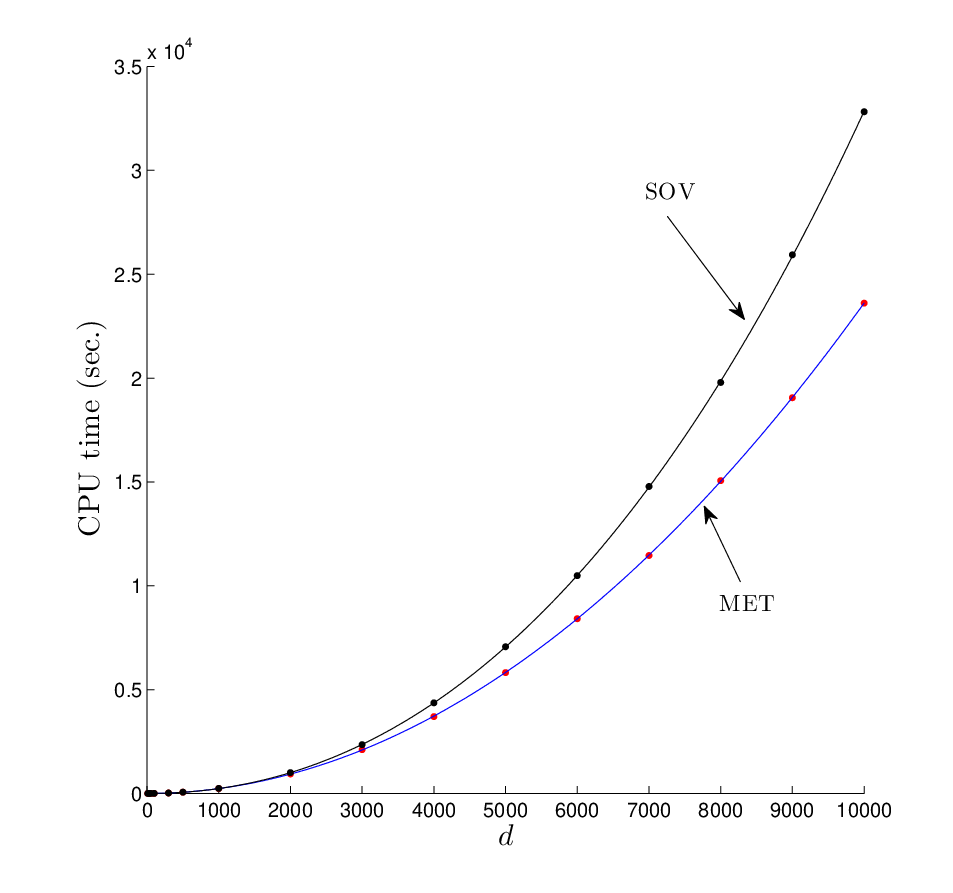
Figure 5 shows the output of a numerical experiment with for various values of . The graph on the left gives the computational cost in seconds. Both the SOV and the MET estimators have cost of — hence the excellent agreement with the least squares cubic polynomials fitted to the empirical CPU data. The table on the right displays the relative error for both methods. In this example, we apply the variable reordering heuristic to the SOV estimator only, illustrating that the heuristic is not always necessary to achieve satisfactory performance with the MET estimator.
| MET | SOV | |
|---|---|---|
| 10 | 0.0063% | 0.0076% |
| 30 | 0.053% | 0.080% |
| 50 | 0.038% | 0.090% |
| 100 | 0.15% | 0.29% |
| 300 | 0.11% | 1.4% |
| 500 | 0.21% | 2.0% |
| 1000 | 0.26% | 3.0% |
| 2000 | 0.18% | 3.9% |
| 3000 | 0.35% | 4.8% |
| 4000 | 0.26% | 8.6% |
| 5000 | 0.33% | 12% |
| 6000 | 0.28% | 7.5% |
| 7000 | 0.21% | 11% |
| 8000 | 0.29% | 8.3% |
| 9000 | 0.28% | 15% |
| 10000 | 0.24% | 12% |
This example confirms the result in Theorem 4.2 that the SOV estimator works better in settings with strongly positive correlation structure (but poorly with negative correlation). Further, the results suggest the MET estimator is also aided by the presence of positive correlation.
5.4 Exact Simulation of Probit Posterior
A popular GLM (Koop et al., 2007) for binary responses with explanatory variables is the probit Bayesian model:
- •
Prior: with and for simplicity ;
- •
Likelihood: .
The challenge is to simulate from the posterior . One can use latent variables (Albert and Chib, 1993) to represent the posterior as the marginal of a truncated multivariate normal. Let be latent variables and define the design matrix . Then, the marginal of the joint pdf
equals the desired posterior . We can thus apply our accept-reject scheme, because the joint is of the desired truncated multivariate form (1) with and

As an numerical example, we apply the probit model to the widely studied extramarital affairs dataset from Koop et al. (2007). The dataset contains independent observations: the binary response indicates if the -th respondent has had an extramarital affair; the six explanatory variables () are male indicator (Male), number of years married (Year), ‘has’ or ‘has not’ children (Kids), religious or not (Relig.), years of formal education (Ed.), and a binary variable denoting whether the marriage is happy or not (Happy). Figure 6 shows the boxplots of the marginal distributions of based on iid simulations from the posterior with prior covariance .
The conclusion that only years of marriage, religiosity, and conjugal happiness are statistically significant is, of course, well known (Koop et al., 2007) and used to validate our new simulation scheme. The question is what have we gained in using minimax tilting?
On the one hand, for the first time we have conducted the Bayesian inference using exact iid samples from the posterior and we did not have to fret about unquantifiable issues such as ‘burn-in’ and ‘mixing-speed’ as is typical with approximate MCMC simulation (Philippe and Robert, 2003).
On the other hand, the acceptance rate in the simulation was , that is, we had to simulate (on average) 217 random vectors to accept one as an exact independent realization from the posterior. Admittedly, this acceptance rate could have been better and as shown in the previous experiments it is going to deteriorate with increasing dimensionality. However, there are hardly any alternatives for exact sampling — naive acceptance rejection for the extramarital data would enjoy an acceptance rate of and without minimax tilting (say, with proposal ) the Accept-Reject Algorithm 2.2 enjoys an acceptance rate of .
Thus, our main point stands: the proposed accept-reject scheme can be used for exact simulation whenever, say , and when is in the thousands it can be used to accelerate Gibbs sampling by grouping or blocking dozens of highly correlated variables together (Chopin, 2011; Philippe and Robert, 2003).
Concluding Remarks
The minimax tilting method can be effective for exact simulation from the truncated multivariate normal distribution. The proposed method permits us to dispense with Gibbs sampling in dimensions less than 100, and for larger dimensions to accelerate existing Gibbs samplers by sampling jointly hundreds of highly correlated variables.
The minimax approach can also be used to estimate normal probability integrals. Theoretically, the method improves on the already excellent SOV estimator and in a tail asymptotic regime it can achieve the best possible efficiency — vanishing relative error. The numerical experiments suggest that the proposed method can be significantly more accurate than the widely used SOV estimator, especially in the tails of the distribution. The experiments also point out to its limitations — as the dimensions get larger and larger it eventually fails.
The minimax tilting approach in this article can be extended to other multivariate densities related to the normal. Upcoming work by the author will argue that significant efficiency gains are also possible in the case of the multivariate student- and general elliptic distributions for which a strong log-concavity property holds. Just as in the multivariate normal case, the approach permits us to estimate accurately hitherto intractable student- probabilities, for which existing estimation schemes exhibit relative error close to 100%.
Acknowledgments
This work was supported by the Australian Research Council under grant DE140100993.
Appendix A Appendix
A.1 Proof of Lemma 3.1
First, we show that is a concave function of for any . To see this, note that if under , then by the well-known properties of log-concave measures (Prékopa, 1973), the function defined as
where is a convex set, is a concave function of . Hence, for an arbitrary linear map , the function defined as is concave as well. It follows that each function
(using the obvious choices of and ) is concave in . Hence, is concave in , because it is a non-negative weighted sum of concave functions.
Second, we show that is convex in for each value of . After some simplification, we can write
Now, each of is convex in , because up to a normalizing constant, this is the cumulant generating function of a standard normal random variable , truncated to . Since a non-negatively weighted sum of convex functions is convex, we conclude that is convex in . Finally, since convexity is preserved under pointwise supremum, is still convex in . Moreover, here we have the strong min-max property: from which the lemma follows.
A.2 Proof of Theorem 4.1
Before proceeding with the proof we note the following.
First, using the necessary and sufficient condition (13), we can write the solution of (12) explicitly as with minimum . In addition, from (13) we can also deduce that and
Second, the asymptotic behavior of has been established by Hashorva and Hüsler (2003). For convenience, we restate their result using our simplified notation.
Proposition A.1 (Hashorva and Hüsler (2003))
Consider the tail probability , where and . Define the set as in (14). Then, the tail behavior of as is
where the constant is given by:
if , and if .
The last two observations pave the way to proving that, depending on the set , either , or . The details of the argument are as follows.
In the setting of Theorem 4.1, the Karusch-Kuhn-Tucker conditions (10) simplify to:
| (17) |
where is a Lagrange multiplier (corresponding to in (10)) and we replaced with .
Case .
We now verify by substitution that, if , the unique solution of (17) is of the asymptotic form
| (18) |
Equation four in (17) is obviously satisfied, because tends to zero by assumption in (18). Next, note that , as . Hence, line three in (17) is also satisfied for sufficiently large :
Next, note that
Hence, from and and Mill’s ratio ( and ) we obtain the asymptotic behavior of :
where we recall that . Equation one in (17) thus simply verifies that
Equation one and two yield , which again is easily verified:
The asymptotic behavior of is obtained by evaluating at the asymptotic solution (18), that is,
| (19) |
It follows from Mill’s ratio, , and that
In other words, from Proposition A.1 we have that as . Therefore,
It follows that for the minimax estimator (11) exhibits vanishing relative error — the best possible asymptotic tail behavior.
Case .
Recall that is the solution of the nonlinear system (8), as well as the optimization program (7) without its constraint (note that a reordering of the variables via the permutation matrix does not change the statement of (7) or (8)). We have , because dropping a constraint in the maximization of (7) cannot reduce the maximum. As in the case of , one can then verify via direct substitution that
is the asymptotic form of the solution to (8). In other words, . Similar manipulations as the ones in (19) lead to . An examination of Proposition A.1 when thus shows that as . In other words, is a bounded relative error estimator for :
A.3 Proof of Theorem 4.2
In the following proof we use the following multidimensional Mill’s ratio (Savage, 1962):
| (20) |
This is a generalization of the well-known one-dimensional result: As in the proof of Theorem 4.1, we proceed to find the asymptotic solution of the nonlinear optimization program (7) by considering the necessary and sufficient Karusch-Kuhn-Tucker conditions (10). In the setup of Theorem 4.2 these conditions simplify to (replacing with ):
| (21) |
We can thus verify via direct substitution that the following
| (22) |
satisfy the equations (21) asymptotically. Equations three and four in (21) are satisfied, because . Let us now examine equations one and two in (21). First, note that from (22)
and hence from the one-dimensional Mill’s ratio we have
In other words, as . It follows that for equation one in (21) we obtain
and for equation two (recall that , so that )
Thus, all of the equations in (21) are satisfied asymptotically and since (21) has a unique solution, we can conclude that . We now proceed to substitute this pair into . Using the one-dimensional Mill’s ratio, , we obtain
As a consequence, using the fact that (recall that is triangular with positive diagonal elements), we have
In other words,
However, by Mill’s ratio (20), we also have
It follows that and the minimax estimator (11) exhibits vanishing relative error:
In contrast, for the SOV estimator we have at most bounded relative error under quite stringent conditions. First, the second moment on the SOV estimator satisfies
and in considering the asymptotics of we are free to select to obtain the best error behavior subject to the constraint . This gives
where is a diagonal matrix such that and . It follows that the relative error of the SOV estimator behaves asymptotically as
A.4 Proof of Corollary 4.1
The corollary follows from a Pinsker-type inequality (Devroye and Györfi, 1985, Page 222, Theorem 2) by observing that (the expectation operator corresponds to the measure ):
where the last equality follows from , which is the case when (11) is a VRE estimator.
A.5 Proof of Lemma 4.1
That is a variational lower bound follows immediately from Jensen’s inequality:
| (23) |
Note that if and , then all the quantities on the left-hand side are available analytically:
| (24) |
Next, we establish the asymptotic behavior of under the conditions of Theorem 4.2. Suppose the pair satisfies and as . Then, , which in combination with , implies . Hence, substituting into (24) and then into the left-hand-side of (23), and simplifying, we obtain
where the last asymptotic equivalence follows from (20). Finally, the convergence of (16) follows by applying the Pinsker-type inequality (Devroye and Györfi, 1985) in conjunction with .
References
- Albert and Chib (1993) Albert, J. H. and S. Chib (1993). Bayesian analysis of binary and polychotomous response data. Journal of the American Statistical Association 88(422), 669–679.
- Azaïs et al. (2010) Azaïs, J.-M., S. Bercu, J.-C. Fort, A. Lagnoux, and P. Lé (2010). Simultaneous confidence bands in curve prediction applied to load curves. Journal of the Royal Statistical Society: Series C (Applied Statistics) 59(5), 889–904.
- Bolin and Lindgren (2015) Bolin, D. and F. Lindgren (2015). Excursion and contour uncertainty regions for latent gaussian models. Journal of the Royal Statistical Society: Series B (Statistical Methodology) 77(1), 85–106.
- Botev et al. (2013) Botev, Z. I., P. L’Ecuyer, and B. Tuffin (2013). Markov chain importance sampling with applications to rare event probability estimation. Statistics and Computing 23(2), 271–285.
- Botts (2013) Botts, C. (2013). An accept-reject algorithm for the positive multivariate normal distribution. Computational Statistics 28(4), 1749–1773.
- Chopin (2011) Chopin, N. (2011). Fast simulation of truncated Gaussian distributions. Statistics and Computing 21(2), 275–288.
- Craig (2008) Craig, P. (2008). A new reconstruction of multivariate normal orthant probabilities. Journal of the Royal Statistical Society: Series B (Statistical Methodology) 70(1), 227–243.
- Davies and Higham (2000) Davies, P. I. and N. J. Higham (2000). Numerically stable generation of correlation matrices and their factors. BIT Numerical Mathematics 40(4), 640–651.
- Devroye and Györfi (1985) Devroye, L. and L. Györfi (1985). Nonparametric density estimation: the L1 view, Volume 119. John Wiley & Sons Inc.
- Fernández et al. (2007) Fernández, P. J., P. A. Ferrari, and S. P. Grynberg (2007). Perfectly random sampling of truncated multinormal distributions. Advances in Applied Probability 39(4), 973–990.
- Galton (1889) Galton, F. (1889). Natural inheritance, Volume 42. Macmillan.
- Gassmann et al. (2002) Gassmann, H., I. Deák, and T. Szántai (2002). Computing multivariate normal probabilities: A new look. Journal of Computational and Graphical Statistics 11(4), 920–949.
- Gassmann (2003) Gassmann, H. I. (2003). Multivariate normal probabilities: implementing an old idea of Plackett’s. Journal of Computational and Graphical Statistics 12(3), 731–752.
- Genton et al. (2011) Genton, M. G., Y. Ma, and H. Sang (2011). On the likelihood function of Gaussian max-stable processes. Biometrika 98(2), 481–488.
- Genz (1992) Genz, A. (1992). Numerical computation of multivariate normal probabilities. Journal of computational and graphical statistics 1(2), 141–149.
- Genz (2004) Genz, A. (2004). Numerical computation of rectangular bivariate and trivariate normal and t probabilities. Statistics and Computing 14(3), 251–260.
- Genz and Bretz (2002) Genz, A. and F. Bretz (2002). Comparison of methods for the computation of multivariate t probabilities. Journal of Computational and Graphical Statistics 11(4), 950–971.
- Genz and Bretz (2009) Genz, A. and F. Bretz (2009). Computation of multivariate normal and t probabilities, Volume 195. Springer.
- Gerber and Chopin (2015) Gerber, M. and N. Chopin (2015). Sequential Quasi-Monte-Carlo sampling. J. R. Statist. Soc. B 77(3), 1–44.
- Geweke (1991) Geweke, J. (1991). Efficient simulation from the multivariate normal and student-t distributions subject to linear constraints and the evaluation of constraint probabilities. In Computing science and statistics: Proceedings of the 23rd symposium on the interface, pp. 571–578. Citeseer.
- Grün and Hornik (2012) Grün, B. and K. Hornik (2012). Modelling human immunodeficiency virus ribonucleic acid levels with finite mixtures for censored longitudinal data. Journal of the Royal Statistical Society: Series C (Applied Statistics) 61(2), 201–218.
- Hajivassiliou and McFadden (1998) Hajivassiliou, V. A. and D. L. McFadden (1998). The method of simulated scores for the estimation of LDV models. Econometrica 66(4), 863–896.
- Hashorva and Hüsler (2003) Hashorva, E. and J. Hüsler (2003). On multivariate gaussian tails. Annals of the Institute of Statistical Mathematics 55(3), 507–522.
- Hayter and Lin (2012) Hayter, A. J. and Y. Lin (2012). The evaluation of two-sided orthant probabilities for a quadrivariate normal distribution. Computational Statistics 27(3), 459–471.
- Hayter and Lin (2013) Hayter, A. J. and Y. Lin (2013). The evaluation of trivariate normal probabilities defined by linear inequalities. Journal of Statistical Computation and Simulation 83(4), 668–676.
- Huser and Davison (2013) Huser, R. and A. C. Davison (2013). Composite likelihood estimation for the Brown–Resnick process. Biometrika 100(2), 511–518.
- Joe (1995) Joe, H. (1995). Approximations to multivariate normal rectangle probabilities based on conditional expectations. Journal of the American Statistical Association 90(431), 957–964.
- Koop et al. (2007) Koop, G., D. J. Poirier, and J. L. Tobias (2007). Bayesian econometric methods, Volume 7. Cambridge University Press.
- Kroese et al. (2011) Kroese, D. P., T. Taimre, and Z. I. Botev (2011). Handbook of Monte Carlo Methods, Volume 706. John Wiley & Sons.
- L’Ecuyer et al. (2010) L’Ecuyer, P., J. H. Blanchet, B. Tuffin, and P. W. Glynn (2010). Asymptotic robustness of estimators in rare-event simulation. ACM Transactions on Modeling and Computer Simulation (TOMACS) 20(1), 6.
- Miwa et al. (2003) Miwa, T., A. J. Hayter, and S. Kuriki (2003). The evaluation of general non-centred orthant probabilities. Journal of the Royal Statistical Society: Series B (Statistical Methodology) 65(1), 223–234.
- Nomura (2014a) Nomura, N. (2014a). Computation of multivariate normal probabilities with polar coordinate systems. Journal of Statistical Computation and Simulation 84(3), 491–512.
- Nomura (2014b) Nomura, N. (2014b). Evaluation of Gaussian orthant probabilities based on orthogonal projections to subspaces. Statistics and Computing, in press.
- Philippe and Robert (2003) Philippe, A. and C. P. Robert (2003). Perfect simulation of positive Gaussian distributions. Statistics and Computing 13(2), 179–186.
- Powell (1970) Powell, M. J. D. (1970). A hybrid method for nonlinear equations. Numerical methods for nonlinear algebraic equations 7, 87–114.
- Prékopa (1973) Prékopa, A. (1973). On logarithmic concave measures and functions. Acta Scientiarum Mathematicarum 34, 335–343.
- Sándor and András (2004) Sándor, Z. and P. András (2004). Alternative sampling methods for estimating multivariate normal probabilities. Journal of Econometrics 120(2), 207–234.
- Savage (1962) Savage, I. R. (1962). Mills’ ratio for multivariate normal distributions. J. Res. Nat. Bur. Standards Sect. B 66, 93–96.
- Tuffin (1999) Tuffin, B. (1999). Bounded normal approximation in simulations of highly reliable markovian systems. Journal of Applied Probability 36(4), 974–986.
- Vijverberg (1997) Vijverberg, W. (1997). Monte Carlo evaluation of multivariate normal probabilities. Journal of Econometrics 76(1), 281–307.
- Wadsworth and Tawn (2014) Wadsworth, J. L. and J. A. Tawn (2014). Efficient inference for spatial extreme value processes associated to log-Gaussian random functions. Biometrika 101(1), 1–15.