AP-Cloud: Adaptive Particle-in-Cloud Method for Optimal Solutions to Vlasov-Poisson Equation

For simplicity of presentation, we consider a second order generalized finite-difference method.

Let $\mathbf{y}^{j}$, $j\in\{1,2,\cdots,m\}$ be the nodes in a neighborhood of reference node $\mathbf{y}^{0}$. Given a $C^{2}$ function $f$, by Taylor expansion we have

where $h$ is the characteristic interparticle distance in the neighborhood, for example, $h=\max\limits_{d,j}|y_{d}^{j}-y_{d}^{0}|$, and $H$ is the Hessian matrix. Putting equations for all neighbors together and omitting higher order term, we obtain

where $V(\mathbf{y}^{0})$ is a generalized Vandermonde matrix, $\partial f(\mathbf{y}^{0})$ is the first order and second order derivative of $f$ at $\mathbf{y}^{0}$, and $\delta f(\mathbf{y}^{0})$ is the increment of $f$.

For example, in 2-D, let $m=5$ and $\delta y_{d}^{j}=y_{d}^{j}-y_{d}^{0}$, then

where $f_{y_{d}}(\mathbf{y}^{0})$ denotes the derivative of $f$ with respect to $y_{d}$, and

To analyze the error in GFD, let $\xi_{d}^{j}=h^{-1}\delta y_{d}^{j}$. Rewrite (7) as

where

Now $V_{0}(\mathbf{y}^{0})$ depends on the shape but not the diameter of the GFD stencil. The error in solving linear system is

The error in right hand size comes from the omitted term in the Taylor expansion $\mathcal{O}(f_{y_{i}y_{j}y_{k}}h^{3})=\mathcal{O}(fh^{3})$ for $i,j,k\in{1,2}$, and $\|V_{0}^{-1}(\mathbf{y}^{0})\|$ is a constant independent of $h$, so the error in $\partial f_{0}(\mathbf{y}^{0})$ is also $\mathcal{O}(fh^{3})$. Because the coefficient before the $l$th order derivative in $\partial f_{0}(\mathbf{y}^{0})$ is $h^{l}$, the error for $l$th order derivative is $\mathcal{O}(fh^{3-l})$

In this example, the number of neighbors is equal to the number of unknowns, and it is quite likely for $V_{0}(\mathbf{y}^{0})$ to be nearly singular. In practice, we use more neighbors in the stencil than the number of coefficients in the Taylor series to improve the stability. In AP-Cloud method, 8 neighbors instead of 5 are used for the second order GFD in two dimensions, and 17 neighbors instead of 9 are used in three dimensions. In this case, the linear system is a least square problem. It is often helpful to assign more weights to closer neighbors to improve the accuracy, which is called the weighted lest square method [8]. AP-Cloud method uses a normalized Gaussian weight function [7]:

where $W$ is the weight, $r$ is the distance of the neighbor from the reference particle, $r_{max}$ is the maximum distance of all neighbors in the stencil from the reference particle, $c=4$.

By solving the linear system or least square problem (7), we can express the gradient $\partial f$ as linear combinations of $\delta f$. For example, once the potential $\phi$ is computed at nodes, we can find its gradient by generalized finite-difference, and then interpolate it to particles by Taylor expansion. Generally, the error of the $k$th order GFD interpolation is $\mathcal{O}(f(\mathbf{y})h^{k+1})$, and its approximation of the $l$th order derivative is $\mathcal{O}(f(\mathbf{y})h^{k-l+1})$.

Given a set of nodes, the selection for GFD neighbors, or the shape of the GFD stencil, is important for both accuracy and stability. Simply choosing the nearest nodes to be neighbors may lead to an imbalanced stencil. We follow the quadrant criterion in [10] and select two nearest nodes from each quadrant to be neighbors.

AP-Cloud also has three steps to calculate the electric field given by a particle distribution: a density estimator, a Poisson solver, and an interpolation step, but each step is different from its counterpart in PIC. Let $\mathcal{C}$ be the set of all computational nodes, and $f(\mathcal{C})=(f(\mathbf{y}^{1}),f(\mathbf{y}^{2}),\cdots,f(\mathbf{y}^{n}))$, where $n$ is the total number of nodes. Below is a detailed description of the three steps.

1. 1.

   Approximate density by interpolating states from particles $\mathcal{P}$ to computational nodes $\mathcal{C}$ by

   			$\displaystyle a(\mathbf{y}^{j})^{T}\partial\tilde{\rho}(\mathbf{y}^{j})$		(16)
   	$\displaystyle:$	$\displaystyle=$	$\displaystyle\sum_{l=0}^{k}\sum_{d_{1},d_{2},\cdots,d_{l}=1}^{D}\underbrace{\frac{1}{h^{D}}\int_{\Omega}\prod_{i=1}^{l}(x_{d_{i}}-y_{d_{i}}^{j})\Phi\left(\frac{\mathbf{x}-\mathbf{y}^{j}}{h}\right)\mathbf{dx}}_{a_{d_{1},d_{2},\cdots,d_{l}}(\mathbf{y}^{j})}\tilde{\rho}_{y_{d_{1}}y_{d_{2}}\cdots y_{d_{l}}}(\mathbf{y}^{j})$
   		$\displaystyle=$	$\displaystyle\underbrace{\frac{1}{h^{D}}\sum_{i=1}^{N}q^{i}\Phi\left(\frac{\mathbf{p}^{i}-\mathbf{y}^{j}}{h}\right)}_{\rho_{M}(\mathbf{y}^{j},h)}.$

   The right hand side of (16) is identical to the Monte Carlo integration in PIC, but the left hand side is a linear combination of derivatives, instead of the simple $\tilde{\rho}(\mathbf{y}^{j},\mathcal{P},h)$ in the PIC method. Because the coefficients in the linear combination, $a(\mathbf{y}^{j})=(a_{d_{1},d_{2},\cdots,d_{l}}(\mathbf{y}^{j}))$, depend only on $h$ and the interpolation kernel, they can be easily pre-calculated and tabulated in a lookup table. The derivatives $\tilde{\rho}_{y_{d_{1}}y_{d_{2}}\cdots y_{d_{l}}}(\mathbf{y}^{j})$ are in turn linear combinations of density values $\rho(\mathbf{y}^{j})$ given by least square solution of (7):

   $$\partial\tilde{\rho}(\mathbf{y}^{j})=V(\mathbf{y}^{j})^{+}\delta\tilde{\rho}(\mathbf{y}^{j}),$$

   (17)

   where $V(\mathbf{y}^{j})^{+}$ is the pseudo-inverse of the Vandermonde matrix.

   Let $C(\mathbf{y}^{j})$ be a matrix such that $\delta\tilde{\rho}(\mathbf{y}^{j})=C(\mathbf{y}^{j})\tilde{\rho}(\mathcal{C})$. Substituting (17) into (16), we get a linear equation for density values at the reference node $\mathbf{y}^{j}$ and its neighors

   $$\underbrace{a(\mathbf{y}^{j})^{T}V(\mathbf{y}^{j})^{+}C(\mathbf{y}^{j})}_{b(\mathbf{y}^{j})}\tilde{\rho}(\mathcal{C})=\rho_{M}(\mathbf{y}^{j},h).$$

   (18)

   Putting equations for all nodes together, we obtain a global linear system for density values

   $$B(\mathcal{C})\tilde{\rho}(\mathcal{C})=\rho_{M}(\mathcal{C},h).$$

   (19)

   where $B(\mathcal{C})=[b(\mathbf{y}^{1});b(\mathbf{y}^{2});\cdots;b(\mathbf{y}^{n})]$. Solution of (19) is the estimated density in AP-Cloud method.

2. 2.

   Discretize the left-hand side of (1) on $\mathcal{C}$ using GFD method. Solve the resulting linear system for $\phi(\mathcal{C})$.

3. 3.

   Obtain the electric field $\mathbf{E}$ by computing $\nabla\phi$ using GFD method, and then interpolating $\phi$ and $\mathbf{E}$ from the $\mathcal{C}$ to $\mathcal{P}$ using a Taylor expansion.

Similar to PIC, the error in AP-Cloud also contains the Monte Carlo noise $\mathcal{E}_{M}$ and the discretization error $\mathcal{E}_{D}$. The Monte Carlo noise in replacing $\bar{\rho}(\mathbf{y}^{j},h)$ by $\rho_{M}(\mathbf{y}^{j},h)$ is identical to the Monte Carlo noise in PIC, that is, $\mathcal{O}(\sqrt{\frac{\rho(\mathbf{y}^{j})}{Nh^{D}}})$. The discretization error in the first step has two sources: the Taylor expansion in (16) and the GFD approximation of the gradient in (17). The difference between the average of the $k$th order Taylor expansion of $\rho$ and $\rho$ itself is $\mathcal{O}(\rho(\mathbf{y}^{j})h^{2\lfloor\frac{k}{2}\rfloor+2})$, where we obtain an additional order for even $k$ due to the symmetry of the kernel $\Phi$. Because the error of $l$th order derivative is $\mathcal{O}(\rho(\mathbf{y}^{j})h^{k-l+1})$, and the coefficient for $l$th order derivative $a_{d_{1},d_{2},\cdots,d_{l}}(\mathbf{y}^{j})=\mathcal{O}(h^{l})$, the discretization error given by the GFD derivative approximation is $\mathcal{O}(\rho(\mathbf{y}^{j})h^{k+1})\geq\mathcal{O}(\rho(\mathbf{y}^{j})h^{2\lfloor\frac{k}{2}\rfloor+2})$. Thus the total discretization error in step 1 is $\mathcal{O}(\rho(\mathbf{y}^{j})h^{k+1})$.

Generalized finite-difference Poisson solver has the same accuracy with its estimation of $\Delta\phi$, i.e., $\mathcal{O}(\rho(\mathbf{y})h^{k-1})$. However, for the second order GFD we observe a supraconvergence when the GFD stencil is well-balanced due to the error cancellation similar to that in the standard five point finite difference stencil. In this case, the error for the solution and its gradient of the GFD Poisson solver are both $\mathcal{O}(f(\mathbf{y})h^{2})$, as observed in our numerical experiments. The interpolation from $\mathcal{C}$ to $\mathcal{P}$, based on the $k$th order Taylor expansion of $\phi$ where the derivatives are given by GFD, is $(k+1)$th order accurate for $\phi$ and $k$th order accurate for $\mathbf{E}$.

Generally, when $k$th order GFD is used in the charge assignment scheme, the Poisson solver, and the differentiation and interpolation routines, the total error for both $\phi$ and $\mathbf{E}$ are

where the $\mathcal{O}(\rho(\mathbf{y})h^{k-1})$ leading term in discretization error is from GFD Poisson solver. To minimize the error, the optimal mesh size is

and the minimized error is

For the second order GFD in particular, we have better error bound due to the symmetry of interpolation kernel and stencil and supraconvergence

and the optimal mesh size is the same as in (5)

The optimal interparticle distance $h$ given in (21) depends on the charge density $\rho$. In most applications, we do not know $\rho$ in advance; otherwise, we do not need the charge assignment scheme to estimate it. We use a Monte Carlo method to obtain a rough estimation of $\rho$:

where $V$ is the volume of a neighborhood of $\mathbf{y}$, and $N^{\prime}$ is the number of particles in the neighborhood.

If the neighborhood is the box with the edge length $h$ centred at $\mathbf{y}$, $V=h^{D}$, we substitute (25) into (21) and obtain

If the charge density undergoes rapid changes, as is typical for certain applications (such as particle accelerators and cosmology), the optimal $h$ (26) also changes rapidly. This causes two potential problems. First, when the difference between levels of refinement on two sides of a cell is too large, that cell cannot find a balanced GFD stencil. If no particle in the coarse side is chosen to be its neighbor, the information on that side is missing. If we force the algorithm to choose a particle on the coarse side as a neighbor, the truncation error from this particle is much larger than that from the others. Second, in some cases, there are almost no particles in the region near the boundary. In order to enforce the boundary condition, interior nodes need to use far away nodes located on the boundary as their neighbors.

To avoid these two problems, we enforce a 2:1 mesh balance. The 2:1 mesh balance requires that the difference between the levels of refinement of two neighbors is at most one. Because the mesh size changes smoothly, both imbalanced GFD stencils and empty regions are avoided.

For clarity, we will focus on the selection of nodes in 3D in this subsection. The selection of nodes in 2D is similar and easier. An octree cell and the centre of a cell will be used interchangeably in this subsection.

We say an octree cell $\mathbf{z}$ is a neighbor of another octree cell $\mathbf{y}$ in a set of octree cells $S$, if

• 1.

  $\mathbf{y},\mathbf{z}\in S$;

• 2.

  $Cell(\mathbf{y})\cap Cell(\mathbf{z})$ is a face.

• 3.

  $level(\mathbf{z})\leq level(\mathbf{y})$;

• 4.

  No ancestor of $\mathbf{z}$ satisfies the previous three conditions.

The neighbors defined here are different from the neighbors in [13] or the neighbors in GFD stencil. Generally, for any cell $\mathbf{y}$ in any set of octree cells $S$, it has at most 6 neighbors, each corresponding to one of its 6 faces. It is possible for a cell to have less than 6 neighbors. For example, root cell has no neighbor in any $S$ in a non-periodic region.

During the selection of nodes, we will keep a queue of octree cells, $Q$, and a list $L(\mathbf{y})$ for each cell $\mathbf{y}$ in $Q$ containing its neighbors in $Q$, which we call neighbor list. The basic operation is to open a cell $\mathbf{y}\in Q$:

1. 1.

   Mark $\mathbf{y}$ as non-node candidate.

2. 2.

   Add all children cells of $\mathbf{y}$ at the end of $Q$, mark them as node candidates.

3. 3.

   Initialize the neighbor lists of the new added cells. Some of the neighbors are their siblings, while others are the neighbors of $\mathbf{y}$ or children of the neighbors of $\mathbf{y}$.

4. 4.

   Update the neighbor lists of the descendent of the neighbors of $\mathbf{y}$.

The algorithm for the selection of nodes is as follows.

1. 1.

   Initialize a queue $Q$, which contains only the root cell.

2. 2.

   Traverse $Q$. For each cell $\mathbf{y}$ in $Q$, test if it satisfies

   $$h<c{N^{\prime}}^{-\frac{1}{2k-2}},$$

   (27)

   where $c$ is a tuning parameter, $h$ is the diameter of the subtree, $n$ is the number of particles in the subtree. If the condition is not satisfied, open $\mathbf{y}$. Let $l$ be the deepest level in $Q$ at the end of this traverse.

3. 3.

   Traverse $Q$. For each leaf cell $\mathbf{y}$ at level $l$, check if the neighbors of $\mathbf{y}$ satisfy the 2:1 mesh balance. Open each neighbor $\mathbf{z}$ that does not satisfy 2:1 mesh balance.

4. 4.

   If $l>0$, let $l\leftarrow l-1$, then repeat step 3. If $l=0$, output all node candidates as computational nodes. If non-periodic boundary condition is used, add additional nodes on the boundary.

Given the number of particles and the order of GFD is fixed, the tuning parameter $c$ in (27) determines the number of nodes. Ideally, $c$ can be computed from the constant in the proportional relationship in (21), which in turn depends on the order of GFD, the kernel function, and the relative magnitude of $\rho$ and its gradients. However, in most applications, the relative magnitude of $\rho$ and its gradients is unknown, so we try different values of $c$ and compare their results to estimate its optimal value in numerical tests.

Checking error balance criterion and 2:1 mesh balance takes only constant number of operations per cell. Except the part to update the neighbor lists, each open operation takes constant number of elementary operations as well, which can be charged on the 8 new added cells, so the time complexity is $\mathcal{O}(|Q|)$, where $|Q|$ is the number of cells in $Q$ in the end of the selection. To analyze the complexity to update the neighbor lists, we note that each time we update the neighbor of a cell $\mathbf{z}$ in $Q$, the level of its neighbor increases. Since the level of its neighbor is bounded by the height of the octree $l_{max}$, the total running time to update neighbors of all particles is $\mathcal{O}(|Q|l_{max})$. Because each interior cell of $Q$ has 8 children, $Q$ is a complete octree, we have $|Q|<8/7n$, where $n$ is the number of not opened cells, i.e., the number of computational nodes. In conclusion, the complexity to select nodes is $\mathcal{O}(|Q|l_{max})$.

After selecting the nodes, the neighbor list can be used to search GFD neighbors. If $\mathbf{z}$ is a neighbor of node $\mathbf{y}$, and $\mathbf{z}$ is not a node itself, then the 4 children of $\mathbf{z}$ that share a face with $\mathbf{y}$ must be nodes because of 2:1 mesh balance. The nodes among the neighbors of $\mathbf{y}$ and the children of these neighbors that share a face with $\mathbf{y}$ are called 1-ring. The union of the $k$-ring and the nodes among the neighbors of $k$-ring nodes and the children of these neighbors that share a face with $k$-ring nodes are called $(k+1)$-ring. GFD neighbors are chosen from 2-ring by the quadrant criterion if there are enough number of nodes in 2-ring. If there are not enough number of nodes in $k$-ring, we will try to select GFD neighbors from $(k+1)$-ring. In our simulations, 5-ring always contains enough neighbors. Because this neighbor searching algorithm only depends on the local nodes information and local data structures, we claim the complexity to search neighbors of a node is independent from the total number of nodes, and this algorithm takes $\mathcal{O}(n)$ time to find neighbors of all computational nodes.

One problem is related to the fact that we do not know in advance how deep the nodes are in the octree while we build the octree. In other words, it is possible that during the algorithm to select nodes, a leaf cell in the octree needs to be opened. However, this is very unlikely to happen in practice, if we always use the maximum depth supported in the implementation. For example, in the 2D Gaussian beam with halo test in Section 5, the order of GFD is 2, the region is $[-1,1]\times[-1,1]$, and the minimum tuning parameter $c$ used in simulations is 0.01. If we use a 64 bits Morton key, the maximum depth of the octree is 21, the cell size of the leaf cell is $(1-(-1))\times 2^{-21}=2^{-20}$. According to (27), $0.01^{2}\times 2^{20\times 2}=1.10\times 10^{8}$ particles must be in the same leaf cell in order to open it, which is more than the total number of particles in the whole domain.

We have performed verification of the Adaptive Particle-in-Cloud method using examples of highly non-uniform distributions of particles typical for accelerator beams with halos. In such problems, a high-intensity, small-sigma particle beam is surrounded by a larger radius halo containing from 3 to 6 orders of magnitude smaller number of particles compared to the main beam. As accurate modeling of realistic accelerator beam and halo distributions is unnecessary for the numerical verification, we represent the system by axially symmetric Gaussian distributions. This also allows us to obtain a benchmark solution.

Consider the following 2D electrostatic problem

where charge density $\rho$ is given by two overlapping Gaussian distribution:

in the domain $\Omega=[-1,1]\times[-1,1]$. We use the following values for the coefficients: the radius of the main beam $\tau_{1}=0.02$, the halo intensity $a_{2}=10^{-5}$, and the width of the halo $\tau_{2}=0.3$. Coefficient $a_{1}=396.1$ is a normalization parameter to ensure $\int_{\Omega}\rho(\mathbf{x})d\mathbf{x}=1$. The model is consistent (in terms of the order of magnitude for the beam versus halo ratio) with real particles beams in accelerators.

While the AP-Cloud method is independent of the geometric shape of the computational domain, we solve the problem in a square domain to enable the comparison with the traditional PIC method. The benchmark solution is obtained in the following way. The problem is embedded in a larger domain, a radius 2 disk, using the same charge density function $\rho$ and the homogeneous Dirichlet boundary condition. A solution, obtained by a highly refined 1D solver in cylindrically symmetric coordinates, is considered as the benchmark solution. The Dirichlet boundary condition for the two-dimensional problem is computed by interpolating the 1D solution at the location of the 2D boundary. This boundary condition function is then used for both the second-order AP-Cloud and PIC methods.

In our numerical simulations, CIC scheme (4) is used in charge assignment and interpolation in PIC method. Theoretically, there are more accurate schemes available, such as triangular shaped cloud with reshaping step. However, these higher order schemes are very computationally intensive, and are not able to give better result than CIC with the same CPU time in our numerical tests. The order of accuracy of AP-Cloud method does not depend on the particular kernel function $\Phi$, so we choose the nearest grid point scheme for its simplicity, that is, $\Phi$ in (16) is set to be the characteristic function of the corresponding octree cell.

Figures 1 - 4 show the distribution of particles coloured according to solution values, nodes, and distributions of errors of the potential and its gradient. $L_{2}$ errors are used in Tables 1 and 2 and Figures 5 and 6 show that the estimation of the potential and its gradient given by AP-Cloud is much more accurate compared to the PIC estimation. For example, the gradient error computed by AP-Cloud with 256 nodes is only about one fourth of the error of PIC with 19077 nodes. Although AP-Cloud is computationally more intensive for the same number of nodes due to the construction of a quadtree and solving an additional linear system for $\rho$, its accuracy under the same running time is still significantly better.

From theoretical complexity analysis in Section 4 and experimental results in Table 3 and Figure 7, the steps of AP-Cloud can be divided into 3 main groups:

• 1.

  Quadtree construction and interpolation, which time complexity is $\mathcal{O}(N\log N)$. The running time for this group is $\mathcal{O}(N\log N)$, which dominates when $N\gg n$.

• 2.

  Searching for nodes, building linear systems and finding interpolation coefficients. The running time for this group is $\mathcal{O}(nl_{max})$, which is small compared to the running time of other two groups.

• 3.

  Solving the linear system for $\rho$ and $\phi$. CPU time depends on both the linear solver and $n$, and dominates for small ratios of $N/n$.

In this test, we did not obtain the second order convergence due to the Monte Carlo noise. Table 4 shows the result of another test, where $\bar{\rho}(\mathbf{y}^{j},h)$ in (2) is given by the integral of the exact density function instead of Monte Carlo integration. The convergence is second order for both the potential and gradient, as expected.

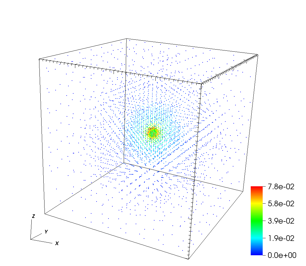
In this Section, we investigate the accuracy of the AP-Cloud method in 3D. To enable comparison with a simple benchmark solution, we study a spherically symmetric extension of the beam-with-halo problem. Despite the loss of physics relevance, it is a useful problem that tests adaptive capabilities of the method. Consider the Poisson equation with the charge density $\rho$ given by two overlapping Gaussian distributions (29) in the domain $\Omega=[-1,1]^{3}$. The radius of center beam is $\tau_{1}=0.02$, the strength of the halo is $a_{2}=10^{-5}$, and the width of the halo is $\tau_{1}=0.3$. The coefficient $a_{1}=7677$ provides the normalization $\int_{\Omega}\rho(\mathbf{x})d\mathbf{x}=1$. The benchmark solution and the boundary condition function were obtained similarly to the 2D case. The distribution of $10^{6}$ particles is shown in Figure 8. The AP-Cloud computation, performed using 4067 nodes (Figure 9), gives a solution with the normalized norm of $\phi$ on particles is 0.0352 ($\|\phi\|_{\infty}=3.038$), and the normalized norm of $\phi_{x}$ on particles is 0.578 ($\|\phi_{x}\|_{\infty}=41.18$).

Results presented in Tables 5 and 6 and Figures 12 and 13 show that the advantage of AP-Cloud is more evident in 3D problem. With only 1546 nodes and less than 1 second running time, AP-Cloud has more accurate result than PIC with 4096000 cells and more than 361 seconds running time.

As mentioned in the introduction, Vlasov-Poisson problems with highly non-uniform distributions of matter can be solved using the adaptive mesh refinement technique for PIC [4, 5]. However, it is well known that AMR-PIC introduces significant artifacts in the form of artificial image particles across boundaries between coarse and fine meshes. These images introduce spurious forces that may potentially alter the particle motion to an unacceptable level [4, 5]. Methods for the mitigation of the spurious forces have been designed in [6]. The traditional PIC on a uniform mesh is free of such artifacts.

The convergence of Adaptive Particle-in-Cloud solutions to benchmark solutions, discussed in the previous Section, already indicates the absence of artifacts. To further verify that AP-Cloud is free of artificial forces present in the original AMR-PIC, we have performed an additional test similar to the one in [4], which involved the motion of a single particle across the coarse and fine mesh interface. For AP-Cloud, we studied the motion of a single test particle represented by a moving cloud of nodes with refined distances towards the test particle. The test particle contained a smooth, sharp, Gaussian-type charge distribution to satisfy the requirements of the GFD method.

The forces and motion of a single test particle obtained with PIC and AP-Cloud methods are shown in Figure 14. We observe that the electric forces computed by the AP-Cloud method are more accurate and smoother compared to even the traditional PIC. But the oscillatory deviation of forces in PIC from the correct direction does not cause accumulation of the total error due to conservative properties of PIC. The trajectories of the particle obtained by both methods are close. The test provides an additional assurance that artificial images are not present in the AP-Cloud method.

References

- [1] R.W. Hockney, J.W. Eastwood, Computer simulation using particles, (CRC Press, 1988), 21.
- [2] H. Johansen, P. Colella, A cartesian grid embedding boundary method for poisson’s equation on irregular domains, J Comput Phys, 1998 (147), 60?85.
- [3] S. Wang, R. Samulyak, T. Guo, An embedded boundary method for parabolic problems with interfaces and application to multi-material systems with phase transitions, Acta Mathematica Scientia, 30B (2010), No. 2, 499 - 521.
- [4] Vay, J-L., et al. “Mesh refinement for particle-in-cell plasma simulations: applications to and benefits for heavy ion fusion." Laser and Particle Beams 20.04 (2002): 569-575.
- [5] Vay, J-L., et al. “Application of adaptive mesh refinement to particle-in-cell simulations of plasmas and beams." Physics of Plasmas (1994-present) 11.5 (2004): 2928-2934.
- [6] Colella, Phillip, and Peter C. Norgaard. “Controlling self-force errors at refinement boundaries for AMR-PIC." Journal of Computational Physics 229.4 (2010): 947-957.
- [7] Onate, E., et al. “A finite point method in computational mechanics. Applications to convective transport and fluid flow." International journal for numerical methods in engineering 39.22 (1996): 3839-3866.
- [8] Benito, J. J., F. Urena, and L. Gavete. “Influence of several factors in the generalized finite difference method." Applied Mathematical Modelling 25.12 (2001): 1039-1053.
- [9] Benito, J. J., et al. “An h-adaptive method in the generalized finite differences." Computer methods in applied mechanics and engineering 192.5 (2003): 735-759.
- [10] Liszka, Tadeusz, and Janusz Orkisz. “The finite difference method at arbitrary irregular grids and its application in applied mechanics." Computers & Structures 11.1 (1980): 83-95.
- [11] Golub, Gene H., and Charles F. Van Loan, Matrix Computations, 4th edition, Johns Hopkins University Press, 2012.
- [12] Barbeiro, S., J. A. Ferreira, and R. D. Grigorieff. “Supraconvergence of a finite difference scheme for solutions in Hs (0, L)." IMA journal of numerical analysis 25.4 (2005): 797-811.
- [13] Zhou, Kun, et al. “Data-parallel octrees for surface reconstruction." Visualization and Computer Graphics, IEEE Transactions on 17.5 (2011): 669-681.
- [14] Cottet, G-H., and P-A. Raviart. "Particle methods for the one-dimensional Vlasov-Poisson equations." SIAM journal on numerical analysis 21.1 (1984): 52-76.
- [15] Wang, Bei, Gregory H. Miller, and Phillip Colella. "A particle-in-cell method with adaptive phase-space remapping for kinetic plasmas." SIAM Journal on Scientific Computing 33.6 (2011): 3509-3537.
Appendix A Error analysis for PIC
Assume the interpolation kernel is symmetric, non-negative, bounded by 1, integrable and normalized over a compact support. That is, for all , for for some , and . These properties hold for all commonly used charge assignment schemes, including the nearest grid point, cloud-in-cell, and triangular shaped cloud schemes without reshaping step. In the following subsections, we will analyze the errors in the three steps of PIC, respectively.
A.1 Error in Step 1
To analyze the error in (2), let us first define an average quantity at a grid point as
Then,
where is analogous to the error in Monte Carlo integration of a continuous function, and is known as moment error or discretization error in step 1, which depends on the interpolation kernel .
A.1.1 Monte Carlo noise
To bound the error , note that the expected value of is