The methodology of resonant equiangular composite quantum gates
Abstract
The creation of composite quantum gates that implement quantum response functions dependent on some parameter of interest is often more of an art than a science. Through inspired design, a sequence of primitive gates also depending on can engineer a highly nontrivial that enables myriad precision metrology, spectroscopy, and control techniques. However, discovering new, useful examples of requires great intuition to perceive the possibilities, and often brute-force to find optimal implementations. We present a systematic and efficient methodology for composite gate design of arbitrary length, where phase-controlled primitive gates all rotating by act on a single spin. We fully characterize the realizable family of , provide an efficient algorithm that decomposes a choice of into its shortest sequence of gates, and show how to efficiently choose an achievable that for fixed , is an optimal approximation to objective functions on its quadratures. A strong connection is forged with classical discrete-time signal processing, allowing us to swiftly construct, as examples, compensated gates with optimal bandwidth that implement arbitrary single spin rotations with sub-wavelength spatial selectivity.
pacs
03.67.Ac, 03.67.Lx, 82.56.Jn, 84.30.VnI Introduction
Composite quantum gates [1, 2] are indispensable to many important quantum technologies, such as nuclear magnetic resonance, magnetic resonance imaging, quantum sensing, and quantum computation [3]. Their versatility arises from cunningly chosen sequences of primitive quantum gates that produce an effective quantum gate with a more desirable dependence on some parameters of interest , such as drive amplitude or background magnetic fields. As a function of , the quantum response function can be tailored to amplify weak signals beyond the statistics of repetition, and suppress noise without measurement. Finding such useful composite gates is thus the subject of intense research.
Even in single spin systems, the focus of this work, extraordinary richness can be found in the possible forms of . For example: NMR spectroscopy, where minute chemical shifts are made clearer through [4, 2, 5]; Heisenberg-limited quantum imaging, where is made sensitive to sub-wavelength position variations [6] without aliasing [7, 8]; sub-wavelength spatial addressing where arbitrary quantum gates with low crosstalk are applied on spin arrays [9, 10, 8]; quantum phase estimation for atomic clocks [11] or tomography [12], where extremely small drifts are amplified by factor in the gradient of ; error-compensation, where fractional control errors are exponentially suppressed like [13, 14, 15, 16, 17, 18, 19, 20]; quantum algorithms such as amplitude amplification [21, 22] where a computation proceeds with input . The discovery of other applications would be expedited if a useful characterization of all achievable could be found.
However, the road to new results does not end with a choice of . Given some reasonable system-dependent quantum control [23], its realization as a composite gate must be found. Only with rare exceptions [16, 9, 8] and great effort are optimal, arbitrary length examples found in closed-form. Thus celebrated techniques including gradient ascent algorithms [5] and pseudospectral methods [24, 25] formulate this as a systematic optimization problem that can be solved by brute force, but unfortunately with an exponential worst-case runtime for finding optimally short approximations. Finding efficient solutions to various control problems would expand the potential of long composite gates, for which the most sophisticated quantum response functions can be constructed.
A tantalizing similarity is seen in discrete-time signal processing [26]. Optimal finite-impulse response filters [27] can be designed simply by choosing the lowest-degree polynomial that is the optimal approximation to a desired frequency response, from which an optimal and exact implementation is computed – made possible by efficient algorithms for both steps. It is recognized that composite gates implement a filter on physical parameters [20, 28], and the use of polynomials in quantum response functions is well-known [29, 30]. Unfortunately, quantum constraints can render computing these polynomials and their optimal implementation a hard problem. It would be a tremendous advance if efficient solutions to these problems could be found, and even more so if the countless results from the exalted history of classical discrete-time signal processing were transferable to the quantum realm.
One noteworthy step in this direction is the Shinnar-LeRoux algorithm [31, 32] and its refinements [33, 34, 35], which have so far been restricted to the field of magnetic resonance imaging. There, represents the amplitude of background magnetic fields and manifests as an off-resonant rotation. Given otherwise perfect and arbitrary single-spin control, this approach enables the efficient design of by a connection to finite-impulse response filters. Unfortunately, extending the concept to situations with different controls and additional restrictions, particularly the case of on-resonant compensating pulse sequences, appears to have been difficult.
We contribute to this aspiration with a methodology, similar to the Shinnar-LeRoux algorithm, for designing composite gates built from resonant primitive gates acting on a single spin, all rotating by angle , but not necessarily with the same phase. We rigorously characterize the quantum response functions achievable in this manner, prove how we can efficiently choose its form with trigonometric polynomials of degree , and prove how its optimal implementation with the shortest sequence of primitive gates can be efficiently computed. In the process, a connection is made with discrete-time signal processing that allows us to inherit some of its machinery. These powerful tools expedite composite gate design, which we demonstrate with three optimal important examples: (1) narrowband and broadband composite population inversion gates; (2) compensated NOT gates with optimal bandwidth; (3) spatially-selective arbitrary single spin rotations below the diffraction limit.
We elucidate in Sec. II the controls available to our single qubit system and demonstrate how equiangular composite gates motivate in Sec. III the intuitive concept of choosing polynomials to explicitly define the quantum response function . This is made rigorous and tractable in Sec. III.1 by a simple characterization of the space of achievable , and showing in Sec. III.2 how an optimal implementation of any such can be efficiently computed. We then show in Sec. III.3 how an achievable can be efficiently computed from a partial specification with polynomials that describe only the composite gate fidelity or transition probability response functions. This enables in Sec. III.4 the efficient design of achievable by inheriting from discrete-time signal processing existing polynomials and efficient polynomial design algorithms. Together, these provide a methodology outlined in Sec. III.5 for the systematic and efficient design of composite quantum gates. Use of this methodology is demonstrated in Sec. IV with the creation of optimal bandwidth compensated gates in Sec. IV.2 that provide an optimal solution in Sec. IV.3 to the problem of implementing sub-wavelength spatially selective arbitrary quantum gates. Further directions are discussed in Sec.V.
II Model
The unitary quantum response function describes how a quantum system evolves under the influence of some parameter of interest. We consider the generic system of a resonantly driven single spin, and present a construction for composite quantum gates that motivates a powerful approach for designing their implemented response functions.
A two-level system driven by time-dependent Rabi frequency and phase is controlled by the Hamiltonian , where and are Pauli matrices. Taking to be constant over time , we generate the primitive rotation
| (1) |
Note that might only be partially under our control and thus contain an uncontrollable residual signal. Our parameter of interest is thus , which captures both effects.
An equiangular composite gate of length is built from these primitive rotations, each with the same rotation amplitude , but with varying phases . This produces a -dependent unitary , or quantum response function, of the form
| (2) | ||||
where , and the phase sums are defined through the recurrence [19]
| (3) | ||||
performed over , then .
Now, we make the crucial observation that is polynomial of degree in and with a particularly elegant representation. Using the trigonometric relation , has the form
| (4) |
where are polynomials of degree at most with coefficients () respectively. In the following, without arguments are understood to be functions of the seen in Eq. 4. As the tuple is an equivalent representation of , we refer to both interchangeably. In particular, achievable tuples are those than can be realized by some composite gate of Eq. 2:
Definition 1 (Achievable polynomial tuples).
A tuple of polynomials is achievable if s.t. has the form of Eq. 4.
We are often interested in only a few components of . For example, the partial tuple fully defines the gate fidelity response function with respect to some target gate .
| (5) |
Similarly, or fully defines the transition probability response function ,
| (6) |
We refer to a tuple with empty slots as an -partial tuple. An -partial tuple is achievable if it is consistent with some achievable tuple.
A brute-force approach to composite gate design is minimizing an objective function for over a space . Though useful examples have been discovered in this manner, such an approach is highly unappealing. In addition to being inefficient with a runtime , there is no guarantee that a globally optimal solution will be found. Furthermore, the procedure provides little of the necessary insight into possible for envisioning further novel applications.
III Systematic and efficient design of optimal composite gates
The functional form of hints at a powerful methodology for composite gate design via choices of the polynomials of degree . This ambition must solve long-standing problems:
- (P1)
-
An insightful characterization of achievable to eliminate the traditional guesswork in envisioning novel quantum response functions and their dependence on .
- (P2)
-
An efficient algorithm to compute the optimal implementing an achievable , in contrast to the intractable random search in time of current state-of-art [8].
- (P3)
- (P4)
-
An efficient algorithm for computing achievable partial tuples optimal for some objective function.
Our main technical advances are precisely the resolution of problems (1-4). We describe in a simple and intuitive manner the set of achievable , and provide efficient algorithms for solving what has traditionally been the hardest aspects of composite gate design. In particular, a beautiful connection is made with the historic field of discrete-time signal processing that allows allows us to inherit much of its prior work in polynomial design. In this manner, the inspired art of composite gates is transformed into a systematic science. Optimal composite gates are simply polynomials optimal for the objective function, and these polynomials can be found efficiently.
III.1 Characterization of quantum response functions
We characterize here achievable choices of quantum response functions in a manner independent of , hence resolving problem (P1). By providing insight into the forms of possible , we also obtain a quantitative explanation for the remarkable versatility of composite gates. Achievability constraints on the polynomials are as follows:
Theorem 1 (Achievable tuples).
A tuple of polynomials of degree at most is achievable iff all the following are true:
(1) are real.
(2) or .
(3)
(4)
Proof.
In forward direction, (1) and (3) are true by applying the trigonometric substitution in Eq. 2 and collecting coefficients of . (2) is true as in Eq. 2. (4) is true as is unitary so and evaluated via Eq. 4 produces
In the reverse direction, we need to show that any satisfying (1-4) is achievable in the sense of Def. 1. We leave these steps to Lem. 1. ∎
Conditions (1-4) for achievable appear fairly general, which allows for great flexibility in choosing arbitrary response functions. They are also understandable and intuitive. A characterization of achievable partial tuples is also useful. Not all quadratures of might be relevant to an objective function, and optimizing over a subset could be easier. In the following, we examine how the unitarity constraint of condition (4) is weakened for all possible -partial tuples.
Theorem 2 (Achievable -partial tuples).
Assuming satisfy conditions (1-3) of Thm. 1,
(1) , is achievable iff
(1a)
(2) , is achievable iff
(2a)
(3) is achievable iff
(3a) , and
(3b) , and
(3c) .
(4) is achievable iff
(4a) and
(4b) .
Proof.
In the forward direction, all the (a) conditions are true from Eq. III.1 using the fact that are all real, hence their squares are positive. (3b) is true by considering Eq. III.1 with the substitution , and computing . Note that the here are complex. Using the odd/even symmetry of , the RHS factorizes into a positive term times or . This is negative so . (3c) is similarly proven by considering . The RHS factorizes into and a positive term. (4b) is proven with the substitution and by considering . In the reverse direction, we need to show that assuming these conditions enable the computation of an achievable . We leave these steps to Lems. 2. 3. ∎
Note that are interchangeable in Thm. 2 as their constraints in Thm. 1 are identical. We also characterize all possible -partial tuples.
Theorem 3 (Achievable -partial tuples).
Assuming satisfy conditions (1-3) of Thm. 1, the following are achievable under their respective conditions
(1) iff .
(2) iff .
(3) iff
(4) iff
Proof.
These simple characterizations show how one can in principle encode almost any arbitrary desired function into quadratures of . Consider , which aside from symmetry and , only needs to satisfy . The famous Stone-Weierstrass theorem [36] assures us that of sufficiently large degree can approximate arbitrarily well any arbitrary continuous real function that satisfies these constrains on the interval . This ability to create almost arbitrary quantum response functions helps explain the applicability of composite gates to many diverse problems.
III.2 Implementation of quantum response functions
Unleashing the potential of arbitrarily sophisticated choices of achievable requires an efficient computation of their implementation . It is clear that the a random search is wholly inadequate as the degree of could be very large. Nevertheless, achievability leads to a certain structure that resolves this problem (P2). This is encapsulated in the following lemma, which is proven constructively and furnishes the reverse direction proof of Thm. 1.
Lemma 1 (Optimal quantum response compilation).
Exactly phases are required to implement an achievable of degree at most , and these phases can be computed in time .
Proof.
A minimum of phases are required to implement a given of degree at most as each application of only increases the degree of by one. We now show that can be implemented with at most phases . Due to the even/odd symmetry of real from Thm. 1 conditions (1) and (3), we can compute its unique phase sum representation in Eq. 2 via the invertible transformation
| (9) |
Let us take the ansatz where is unitary and as represents a unitary from Thm. 1 condition (4). Thus also has a phase sum representation . These two phase sums are related by the linear map of Eq. 3, with inverse
| (10) |
By choosing
| (11) |
we satisfy the necessary condition from Eq. 3. In particular, is real, as Eq. III.1 has the trailing term . Hence the RHS of Eq. 11 has absolute value . By recursively reducing the degree of , we obtain all phases . The terminal case at must be consistent with Eq. 3 where . When evaluated with Eq. 9, 10, this is satisfied only if (Thm. 1 condition (2)), which is true for achievable . All steps in this procedure can be computed in time , and there are only recursions, leading to a runtime of . ∎
III.3 Computation of quantum response functions
A consequence of Lem. 1 is that designing a composite gate is no more difficult than finding the to describe the quantum response function . Optimizing for some objective function is far more intuitive than the prior art of a random search over . However, this still is a difficult problem. The unitary constraint Eq. III.1 represents a system of quadratic multinomial equations that would have to be solved at each step of the optimization to obtain an achievable . Solving such systems is in general an NP-complete task. This is the essence of problem (P3): it would be much easier to optimize a subset of , and doing so is often the problem of practical interest anyway.
This subset optimization is illustrated by the response functions , of Eq. 5,6 which depend on only two polynomials. Optimizing just these for some objective function offers more freedom as the unitary constraint Eq. III.1 is weakened to that of Thm. 2. Ultimately, we must compute some achievable from a partial specification in order to find the phases .
Fortunately, the structure of achievable partial tuples can be exploited to derive algorithms analogous to prior art [31] based on polynomial sum-of-squares problems [37], but specialized to the symmetries of Thm. 2. We present results for , of odd degree and show how they apply to all achievable -partial tuple. As these primarily serve to show that the necessary conditions in Thms. 1, 2, 3 are also sufficient, the details of the proofs for Lems. 2, 3, which also furnish constructive algorithms for computing from partial tuples, may be skipped by the casual reader.
Lemma 2 (Transition probability sum-of-squares).
Proof.
Consider the polynomial of degree at most
| (12) |
with roots ( contains duplicates if a root is degenerate). Since , are odd polynomials, is real for all real . Because is real, complex roots occur in pairs. Thus we can group subsets of without loss of generality as:
| (13) | ||||
Observe that are real, and is complex. Thus
| (14) |
with scale constant . Using (3b), . Hence, all negative roots in occur with even multiplicity. Using (3a), . As changes sign at , is odd. Using the oddness of , . Since , all positive roots in occur with even multiplicity. Thus, all real roots excluding occur with even multiplicity. By repeated application of the two-squares identity
| (15) |
the complex factors can be simplified like
| (16) |
where are real polynomials in . Thus where
| (17) |
and are odd real polynomials of degree at most . Note that different choices of signs Eq. 15 generates a finite number of different valid solutions. Computing the roots of is the most difficult step of this algorithm, but can be done in time [38]. ∎
The proof for even , and tuples carries through with minor modification. The stated conditions in Thm. 2 guarantee that the various factors of , necessary for the correct symmetry of the unspecified polynomials occur with the right multiplicity, and that all other real roots occur with even multiplicity. Some additional processing for the case is required as the output is not guaranteed to satisfy . However, is still true so by computing , we can form an achievable .
We now present the analogous algorithm for .
Lemma 3 (Fidelity response sum-of-squares).
Proof.
With the Weierstrass substitution , define the real polynomials
| (18) |
These polynomials have extremely useful symmetries which we indicate with angled brackets . are Even aNtipalindromes while are Odd Palindromes . Antipalindromes satisfy whereas palindromes satisfy . Note that , and , polynomials with multiplication form a group isomorphic to . For example, .
Consider the positive, palindromic polynomial
| (19) |
with scale constant , and roots , where is the multiplicity of the zero roots. Note the degree of is , not , because the first coefficients being zero implies the last are as well. Due to the symmetry of , roots , roots ,, and . Thus we group subsets of these roots without any loss of information as follows:
| (20) | ||||
Observe that are real, are imaginary and are complex. From the real roots, we construct the factor
| (21) |
The positiveness of means that all real factors have even multiplicity. Thus is a polynomial. From the complex roots, we form
| (22) | ||||
The symmetry of terms under the squares is one of , and occur in a combination that forms a group under repeated application of the two-squares identity of Eq. 15. Thus we can construct
| (23) | ||||
For some combinations of multiplicities, this decomposition will not produce polynomials with the symmetry required by , . However, summing the multiplicities of these roots shows that is even and that such combinations do not exist. From this decomposition, we compute using
| (24) | ||||
As with Lem. 2, different choices of signs in the two-squares identity lead to multiple valid solutions. Computing the roots of is the still most difficult step, but can be done in time . ∎
The case of even replaces Eq. 19 with and we find with and with symmetry . A similar root counting argument guarantees the existence of such solutions. The coefficients of are then computed also using Eq. 24. This procedure carries through without modification for the other tuples (1), (2) of Thm. 2.
III.4 Selection of quantum response functions
It should be clear that optimal composite gate design is a systematic process no more difficult than choosing one or two polynomials optimal for some objective function. Nevertheless, problem (P4) is that computing these optimal polynomials could still be a difficult task. However, the constraints on achievable partial tuples in Thms. 2, 3 seem fairly lax, which lends hope that this could be done efficiently. In fact these constraints are consistent with textbook problems in approximation theory [39].
It is at this point where a close connection with discrete-time signal processing [26] is made. Efficient algorithms [40, 41, 42, 43, 44] for designing polynomials optimal for arbitrary objective functions under a variety of optimality criteria have been extensively studied for finite-impulse response filters [27]. We thus inherit much of this machinery, and in many cases, existing polynomials consistent with achievability have already been found and are directly transferable.
A most common optimality criterion is the Chebyshev norm: Let be the objective function, with continuous weight function , to be approximated by a polynomial of degree on a bounded subset of the closed interval with the smallest Chebyshev error norm
| (25) |
The unique best approximation can be computed efficiently by Remez-type exchange algorithms [45]. Many variants exist such as where is a trigonometric polynomial [40], bounded [42], subject other unary or linear constraint [43], and even complex [41]. Linear programming methods [43] provide an alternate solution. Efficient algorithms for other optimality criteria such as least squares are also available [46, 47].
These algorithms efficiently solve the problem of optimization over achievable quantum response functions where the objective functions are -partial or -partial tuples. Optimization for a -partial objective function involves a single quadrature from together with a single real objective function . Thus we optimize over for in Eq. 25 subject to the constraints of Thm. 3 for the corresponding quadrature. The slightly more complicated -partial case instead specifies two quadratures and real objective functions . Thus we define , and optimize over for subject to the constraints of Thm. 2 for the corresponding quadratures. Note that the unitarity inequality constraint poses no difficulty as .
III.5 The methodology of composite quantum gates
Our efforts lead us to a methodology for the design of single spin quantum response functions through composite quantum gates built from a sequence of primitive gates all rotating by , but each with its own phase . The procedure is systematic, flexible, and most importantly, provably efficient:
- Problem statement
-
Given and objective function for either -partial or -partial tuples, find the composite quantum gate that implements through the optimal -approximation to .
- Solution procedure
- (S1)
- (S2)
-
Choose optimality criterion.
–The Chebyshev norm is most common. - (S3)
-
Execute polynomial optimization algorithm over achievable partial tuples.
–Remez-type algorithms are efficient. - (S4)
- (S5)
-
Compute phases .
–This can be done efficiently by Lem. 1.
IV Examples
Using the methodology in Sec. III.5, composite quantum gates with response function that minimize the error with respect to arbitrary objective functions can be efficiently designed. We illustrate this process with three examples of independent scientific interest: compensated population inversion gates, compensated broadband NOT gates, and compensated narrowband quantum gates.
Population inversion gates rotate states to and vice-versa, and come in two flavors. The broadband variant implements this rotation with high probability across the widest bandwidth of , meaning that the transition probability response function from Eq. 6 is close to . The narrowband variant instead implements this rotation with low probability so , except at a single point . We discuss optimal design of these gates in Section IV.1. As closed-form solutions for these gates are already known, and used extensively in NMR spectroscopy, they help build familiarity with the methodology in Sec. III.5 when it is used to solve open questions in the next two examples.
Broadband compensated NOT gates implement the rotation with high fidelity over the widest bandwidth of parameters. Whereas population inversion gates only succeed on initial states to , NOT gates apply a rotation with a known phase for all input states. Such gates have been extensively studied for applying uniform rotations in the presence of drive field inhomogeneities, particularly in quantum computing applications, and our methodology, presented in Sec. IV.2, solves open questions regarding the scaling of bandwidth with sequence length as well as their efficient synthesis.
A complementary design problem addressed in Sec. IV.3 is that of narrowband compensated quantum gates. These instead apply a desired arbitrary rotation at a single value, and the identity rotation elsewhere over widest bandwidth of parameters. Such gates are highly relevant to minimizing crosstalk in the selective addressing of spins in arrays, particularly when spin-spin distances are below the diffraction limit, as might be found in architectures for scalable architectures of ion-trap quantum computation.
IV.1 Composite population inversion gates
Population inversion gates maximize the bandwidth over which the transition probability response function from Eq. 6 is close to for the broadband variant, or close to for the narrowband variant. Note that in both cases, perfect population inversion occurs at for odd, owing to the fact that . Moreover, the optimal polynomials and phases for both variants turn out to be related by a simple transformation, so it suffices for us to consider only the broadband case.
Composite gates with these properties have been studied extensively for nuclear magnetic resonance and quantum computing applications. One approach to obtaining broadband behavior is with the maximally flat ansatz [9]. This exponentially suppresses errors in the transition probability to order , thus over a wide range of . Remarkably, the that implement this profile can be found in closed form [48] with optimal sequence lengths . More recently, a second approach has emerged [8], motivated by the following observation: as the flat ansatz only increases bandwidth indirectly through the suppression order , better results can be obtained by directly optimizing for bandwidth, while ensuring that the worst-case error remained bounded.
The procedure of Sec. III.5 for odd formalizes this task as a straightforward optimization problem:
(S1) Choose the objective function for the 2-partial tuple. Since is close to over , the unitarity constraint implies that a rotation is approximated over , with an unspecified phase that varies with . As consistency with Thm. 1 requires that , this implies that identity is applied at , thus must not contain .
(S2) Choose the Chebyshev optimality criterion, where the best solves the minimax optimization problem
| (26) |
where the worst-case transition probability over is .
(S3) Find the function that solves Eq. 26. For consistency with Thm. 1, the optimization is over real odd polynomials bounded by .
(S4) Using Lem. 2, compute the achievable tuple from the partial specification .
(S5) Compute from using Lem. 1.
The solution to (S3) is the Dolph-Chebyshev window function [49, 50] famous in discrete-time signal processing.
| (27) |
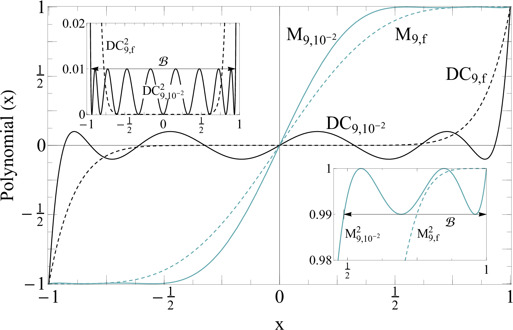
where are Chebyshev polynomials. Note the ripples of bounded by in Fig. 1. This is in contrast to monotonic increase of the limiting function, indicated by the subscript f,
| (28) |
which is maximally flat at , but has significantly narrower bandwidth. Using , the bandwidth in coordinates is to order
| (29) |
Given the same target bandwidth, the worst-case error of is exponentially smaller than . Note also the quadratic difference in the scaling with of the bandwidth over which does not approximate .
| (30) |
The ripples in the amplitude are a generic feature of best polynomial approximations to functions in the Chebyshev norm. By sacrificing flatness, much smaller absolute variations in error can be achieved over some specified bandwidth . This is a common theme that will be revisited in the subsequent example.
IV.2 Broadband compensated NOT gates
Broadband compensated NOT gates maximize the bandwidth over which the fidelity response function with respect to the target gate is close to . One option consistent with this goal is the choice of fidelity response functions that are maximally flat with respect to . When the correction order increases, deviations from are exponentially suppressed, resulting in improved approximations of the target gate over wider ranges of . The central difficulty of this pursuit is finding the phases that maximize for any given . Unlike the population inversion gates of Sec. IV.1, this appears to be significantly more difficult; optimal length solutions for the have only been found in closed-form for small [19].
This problem has been attacked over the course of two decades, starting with Wimperis [13] who found the in closed form for BB1, a sequence with . This was extended by Brown et. al. [15] with SK for arbitrary through a recursive construction, and then by Jones [18, 51] with Fn to in closed-form through sequence concatenation. The most recent effort [19] proved a lower bound of and conjectured that the sequence BB ( in [51]) with is optimal through brute-force up to . Using our methodology, we can easily prove this conjecture and efficiently compute its implementation .
Moreover, our methodology enables a second option. Instead of optimizing for correction order, it is possible to directly minimize the worst-case infidelity , which is the experimental quantity of interest, over a target bandwidth . We find that doing so leads to an improvement in that scales exponentially with over the maximally flat case. To prove these statements, we proceed with the design outline of Sec. III.5 for odd :
(S1) Choose the objective function for the 3-partial tuple. Provided that does not contain the point , this is consistent with the constraints of Thm. 3. This corresponds to finding a fidelity response function that is close to across .
(S2) The best fidelity response function for the maximally flat approach in prior art is obtained from the function that maximizes the correction order
| (32) | ||||
where is the worst-case infidelity over the bandwidth . It is easy to verify that any such satisfies . The more direct approach uses the Chebyshev optimality criterion, where the best solves the minimax optimization problem
| (33) |
(S3) Find the function that solves Eqs. 32, 33. For consistency with Thm. 1, the optimization is over real, odd polynomials bounded by .
(S4) Using Lem. 3, compute the achievable tuple from the partial specification .
(S5) Compute from using Lem. 1.
We now present the solutions to (S3) of this procedure. This is the most difficult step, as once is provided, the implementation is a straightforward calculation. Eq. 32 is solved by the the odd polynomial that satisfies the following independent linear constraints:
| (34) |
As a degree odd polynomial has free parameters, a degree polynomial is necessary and sufficient. This is solved by the polynomial
| (35) |
with an example plotted in Fig. 1. The index indicates the degree, and the subscript f indicates that this is a maximally flat polynomial. As is monotonically decreasing from , the relation between infidelity and bandwidth is obtained by solving to leading order:
| (36) |
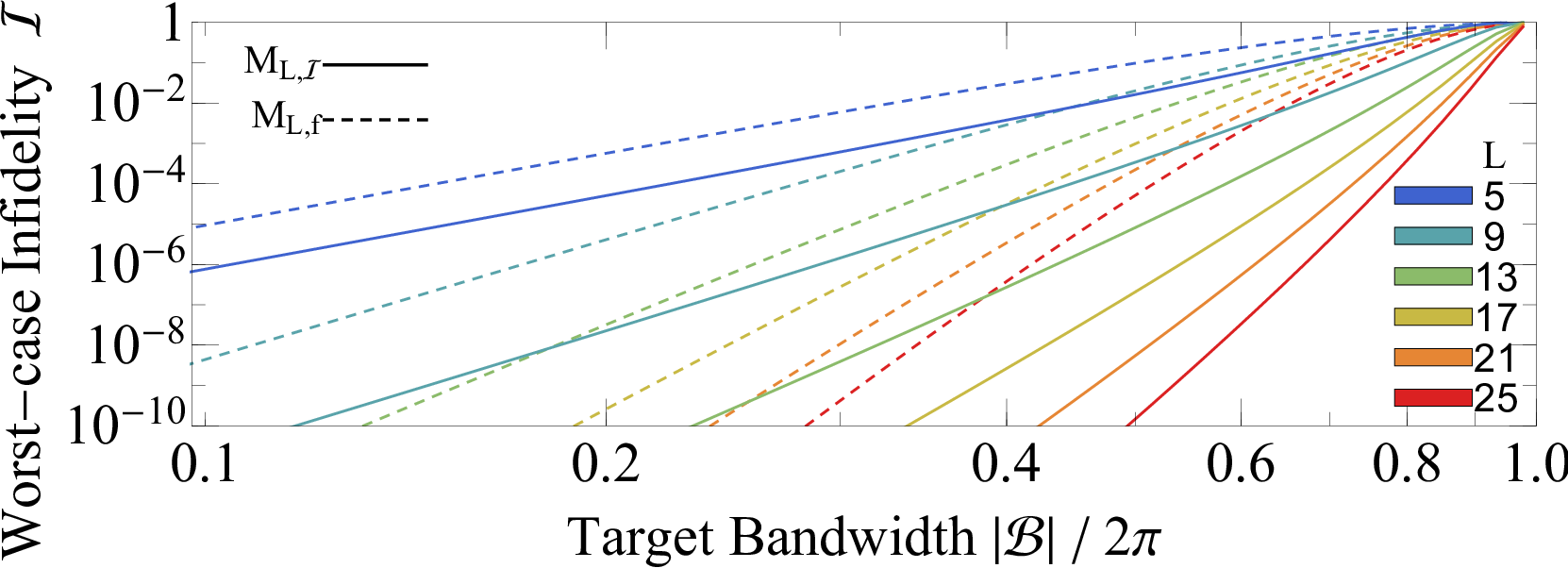
Thus given some target bandwidth of high-fidelity operation, the composite quantum gate represented by implements NOT with a worst-case fidelity that decreases exponentially with sequence length. This proves the conjecture of [19].
The odd polynomials of degree that satisfy the Chebyshev error norm optimality criterion in Eq. 33 can also be found. We label these polynomials , where indicates the degree, and is the worst-case infidelity, which is directly related to the bandwidth . For , we have a complicated looking expression
| (37) |
parameterized implicitly through . For larger , such as in Fig. 1, the can always be computed numerically through the famous Parks–McClellan algorithm [40] for finite impulse response filters. Remarkably, the Chebyshev error of this approximation problem is known [52]:
| (38) | ||||
By comparing Eqs. 36. 38 in Fig. 2, it can be seen that for any target and sequence length , the composite quantum gate has a worst-case infidelity that improves on by an exponential factor .
| where | ||
|---|---|---|
| Eq. 37 | ||
In contrast to the BB sequences that are fixed for each , OB allows for an optimal design trade-off between bandwidth and infidelity . As seen in Fig. 1, this occurs by introducing equiripples of equal amplitude bounded by , similar to the DCL,I polynomials for population inversion gates. Thus, given the same performance targets, an extremely short OB gate can perform just as well as a significantly longer BB gate. In other words, maximizing the correction order only improves the achieved bandwidth indirectly, leading to a poor trade-off between and , whereas better results are naturally achieved by optimizing for polynomials that directly solve Eq. 33 by minimizing infidelity over a target bandwidth.
IV.3 Composite quantum gates with sub-wavelength spatial selectivity
Narrowband compensated gates maximize the bandwidth over which the fidelity response function with respect to identity is close to , except at a single point where an arbitrary target rotation is applied. Although the direct approach is computing new polynomials that satisfy these properties, we can reuse the polynomials from Sec. IV.2 by making certain assumptions on the physical system. In the following, we also assume that .
Consider a Gaussian beam of fixed width . As a function of position , this beam has a spatially-varying Rabi frequency . Thus when applied for time , a primitive gate that also varies as a function of position is generated, where and . At , one can choose such that the target rotation is implemented, and due to exponential decay of the Gaussian beam, moving away from the beam center approximates the identity gate with infidelity . Thus at distance from the beam center, the worst-case infidelity is . As the minimum possible beam width is the wavelength of light, selective addressing below the diffraction limit appears impossible. However, even this can be overcome with a carefully designed composite quantum gate.
Narrowband composite gates of length applicable to this scenario have been widely studied. For instance, [13, 10] report beam width reductions by factor [13, 10]. Further reduction is possible with longer composite gates [19], but with poor scaling .
A better narrowband composite gate results from using the broadband identity gate designed from the polynomial in presented in Sec. IV.2. Then, the fidelity response function with respect to identity is , which, as we now show, corresponds to a quadratic improvement of .
Let us compose ID with the Gaussian beam to produce the spatially-varying quantum response function
| (39) |
for some choice . Note that is stable with respect to beam-pointing errors in due to the vanishing first derivative. The degree of spatial selectivity is computed from the bandwidth in Eq. 38 by substituting and solving for . Thus, identity is implemented with infidelity at most at all as seen in Fig. 3, where to leading order ,
| (40) |
Meanwhile at , we obtain the gate
| (41) |
where . The desired rotation is thus obtained by choosing such that and rotating all phases , which follows from .

| where | ||
|---|---|---|
| Eq. 37 | ||
The optimality of these results follows from the construction of as optimal bandwidth polynomials. In particular, using the flat polynomial leads to the scaling found in prior art and Fig. 3(inset).
V Conclusion
We have presented and applied a methodology, analogous to the Shinnar-LeRoux algorithm but with different controls, for the systematic design of resonant equiangular composite quantum gates of length on a single spin. In particular, we show that all steps are efficient with time complexity , and provide an extremely rigorous characterization of achievable quantum response functions. Moreover, the elegant and practical connection made with discrete-time signal processing allows us to inherit and adapt many existing algorithms and polynomials used in the design of classical response functions for this quantum problem. Much potential remains untapped there, and interdisciplinary exchange could spur the discovery of further connections, leading to the development of previously intractable applications. Indeed, this relationship has already proven fruitful in surprising directions, such as recent work furnishing optimal algorithms for important problems such as Hamiltonian simulation [53, 54] on a quantum computer.
In fact, our work bridges discrete-time signal processing and quantum query algorithms for evaluating symmetric boolean functions. The idea here is that the space of a single-qubit, as we study here, is isomorphic to the subspace spanned by a uniform superposition of marked states and a uniform superposition of unmarked state in such a query problem. Query algorithms can be built to calculate a boolean function that depends only on the number of marked states (i.e. for some ) and do so with a Grover-type algorithm of partial reflections (e.g. [55, 21, 56, 57]). Thus, the same methods introduced here also give a way to determine how many reflections (analogous to our ) and what reflections (analogous to our ) are required to compute any particular symmetric boolean function, achieving the known lower bounds for this problem, which (not) coincidentally are also derived using polynomials [58]. As examples of this correspondence, is an optimal solution for OR [22], is optimal for Majority.
Various thought provoking extensions are also motivated. The set of achievable quantum response functions is changed by introducing elements such as additional (possibly continuous) control parameters, disturbances, coupled spins [59, 10, 60], or open systems [61, 20]. These all enable their own unique applications, but also appear difficult to solve somehow systematically and intuitively. Our success in the case of composite gates contributes supporting evidence that a useful characterization as well as efficient methods for these more complex design problems could exist.
VI Acknowledgements
G.H.Low acknowledges funding by NSF RQCC Project No.1111337 and NRO. T.J.Yoder acknowledges funding by NDSEG. We thank Alan Oppenheim and Tom Baran for inspiring discussions, and connections made possible by their 6.341x open online MITx course. We thank Yuan Su for useful comments on the paper.
References
- [1] L. M. K. Vandersypen and I. L. Chuang, “NMR techniques for quantum control and computation,” Rev. Mod. Phys. 76, 1037–1069 (2005).
- [2] R Freeman, Spin choreography (Oxford University Press Oxford, UK, 1998).
- [3] Michael A. Nielsen and Isaac L. Chuang, Quantum Computation and Quantum Information, 1st ed. (Cambridge University Press, 2004).
- [4] Malcolm H. Levitt, “Composite pulses,” in eMagRes (John Wiley & Sons, Ltd, 2007).
- [5] Navin Khaneja, Timo Reiss, Cindie Kehlet, Thomas Schulte-Herbrüggen, and Steffen J. Glaser, “Optimal control of coupled spin dynamics: design of NMR pulse sequences by gradient ascent algorithms,” J. Mag. Res. 172, 296 – 305 (2005).
- [6] K. Arai, C. Belthangady, H. Zhang, N. Bar-Gill, S. J., DeVience, P. Cappellaro, A. Yacoby, and R. L., Walsworth, “Fourier magnetic imaging with nanoscale resolution and compressed sensing speed-up using electronic spins in diamond,” Nat. Nano 10, 859–864 (2015).
- [7] T. Häberle, D. Schmid-Lorch, K. Karrai, F. Reinhard, and J. Wrachtrup, “High-dynamic-range imaging of nanoscale magnetic fields using optimal control of a single qubit,” Phys. Rev. Lett. 111, 170801 (2013).
- [8] Guang Hao Low, Theodore J. Yoder, and Isaac L. Chuang, “Quantum imaging by coherent enhancement,” Phys. Rev. Lett. 114, 100801 (2015).
- [9] Boyan T. Torosov and Nikolay V. Vitanov, “Smooth composite pulses for high-fidelity quantum information processing,” Phys. Rev. A 83, 053420 (2011).
- [10] J. T. Merrill, S. C. Doret, Grahame Vittorini, J. P. Addison, and Kenneth R. Brown, “Transformed composite sequences for improved qubit addressing,” Phys. Rev. A 90, 040301 (2014).
- [11] J. Vanier, “Atomic clocks based on coherent population trapping: a review,” App. Phys. B 81, 421–442 (2005).
- [12] Shelby Kimmel, Guang Hao Low, and Theodore J. Yoder, “Robust calibration of a universal single-qubit gate set via robust phase estimation,” Phys. Rev. A 92, 062315 (2015).
- [13] S. Wimperis, “Broadband, narrowband, and passband composite pulses for use in advanced NMR experiments,” J. Mag. Res., Series A 109, 221 – 231 (1994).
- [14] Holly K. Cummins, Gavin Llewellyn, and Jonathan A. Jones, “Tackling systematic errors in quantum logic gates with composite rotations,” Phys. Rev. A 67, 042308 (2003).
- [15] Kenneth R. Brown, Aram W. Harrow, and Isaac L. Chuang, “Arbitrarily accurate composite pulse sequences,” Phys. Rev. A 70, 052318 (2004).
- [16] Götz S. Uhrig, “Keeping a quantum bit alive by optimized -pulse sequences,” Phys. Rev. Lett. 98, 100504 (2007).
- [17] Xin Wang, Lev S. Bishop, Edwin Barnes, J. P. Kestner, and S. DasSarma, “Robust quantum gates for singlet-triplet spin qubits using composite pulses,” Phys. Rev. A 89, 022310 (2014).
- [18] Jonathan A. Jones, “Nested composite NOT gates for quantum computation,” Phys. Lett. A 377, 2860 – 2862 (2013).
- [19] Guang Hao Low, Theodore J. Yoder, and Isaac L. Chuang, “Optimal arbitrarily accurate composite pulse sequences,” Phys. Rev. A 89, 022341 (2014).
- [20] A. Soare, H. Ball, D. Hayes, J. Sastrawan, M. C. Jarratt, J. J. McLoughlin, X. Zhen, T. J. Green, and M. J. Biercuk, “Experimental noise filtering by quantum control,” Nat. Phys 10, 825–829 (2014).
- [21] Gilles Brassard, Peter Høyer, and Alain Tapp, “Quantum counting,” in Automata, Languages and Programming (Springer, 1998) pp. 820–831.
- [22] Theodore J. Yoder, Guang Hao Low, and Isaac L. Chuang, “Fixed-point quantum search with an optimal number of queries,” Phys. Rev. Lett. 113, 210501 (2014).
- [23] Steffen J Glaser, Ugo Boscain, Tommaso Calarco, Christiane P Koch, Walter Köckenberger, Ronnie Kosloff, Ilya Kuprov, Burkhard Luy, Sophie Schirmer, Thomas Schulte-Herbrüggen, et al., “Training Schrödinger’s cat: Quantum optimal control,” Eur. Phys. J. D 69, 1–24 (2015).
- [24] J. Ruths and J. S. Li, “Optimal control of inhomogeneous ensembles,” IEEE Trans. Autom. Control 57, 2021–2032 (2012).
- [25] I. Michael Ross and Mark Karpenko, “A review of pseudospectral optimal control: From theory to flight,” Annu. Rev. Control 36, 182 – 197 (2012).
- [26] A.V. Oppenheim and R.W. Schafer, Discrete-time Signal Processing (3rd Ed.), Prentice-Hall signal processing series (Prentice Hall, 2010).
- [27] F.J. Harris, “On the use of windows for harmonic analysis with the discrete Fourier transform,” Proc. IEEE 66, 51–83 (1978).
- [28] Chingiz Kabytayev, Todd J. Green, Kaveh Khodjasteh, Michael J. Biercuk, Lorenza Viola, and Kenneth R. Brown, “Robustness of composite pulses to time-dependent control noise,” Phys. Rev. A 90, 012316 (2014).
- [29] J. S. Li and N. Khaneja, “Ensemble control of Bloch equations,” IEEE Trans. Autom. Control 54, 528–536 (2009).
- [30] J. Shin Li, Justin Ruths, Tsyr Yan Yu, Haribabu Arthanari, and Gerhard Wagner, “Optimal pulse design in quantum control: A unified computational method,” Proc. Natl. Acad. Sci. U.S.A. 108, 1879–1884 (2011).
- [31] Meir Shinnar, Scott Eleff, Harihara Subramanian, and John S. Leigh, “The synthesis of pulse sequences yielding arbitrary magnetization vectors,” Mag. Res. Med. 12, 74–80 (1989).
- [32] J. Pauly, P. Le Roux, D. Nishimura, and A. Macovski, “Parameter relations for the Shinnar-Le Roux selective excitation pulse design algorithm [NMR imaging],” IEEE Trans. Med. Imag. 10, 53–65 (1991).
- [33] Vasiliki N Ikonomidou and George D Sergiadis, “Improved Shinnar-Le Roux algorithm,” J. Mag. Res. 143, 30 – 34 (2000).
- [34] Kuan J. Lee, “General parameter relations for the Shinnar-Le Roux pulse design algorithm,” Journal of Magnetic Resonance 186, 252 – 258 (2007).
- [35] William A. Grissom, Zhipeng Cao, and Mark D. Does, “-selective excitation pulse design using the ShinnarLe Roux algorithm,” Journal of Magnetic Resonance 242, 189 – 196 (2014).
- [36] M. H. Stone, “The generalized Weierstrass approximation theorem,” Mathematics Magazine 21, 167–184 (1948).
- [37] Murray Marshall, Positive polynomials and sums of squares, 146 (American Mathematical Soc., 2008).
- [38] C.Andrew Neff and John H. Reif, “An efficient algorithm for the complex roots problem,” J. Complex 12, 81 – 115 (1996).
- [39] Günter Meinardus, Approximation of functions: Theory and numerical methods, Vol. 13 (Springer Science & Business Media, 2012).
- [40] J. McClellan, T. Parks, and L. Rabiner, “A computer program for designing optimum FIR linear phase digital filters,” IEEE Trans. Audio Electroacoust. 21, 506–526 (1973).
- [41] Lina J. Karam and James H. McClellan, “Chebyshev digital FIR filter design,” Signal Process. 76, 17 – 36 (1999).
- [42] Francis Grenez, “Design of linear or minimum-phase FIR filters by constrained Chebyshev approximation,” Signal Process. 5, 325–332 (1983).
- [43] Mathias Lang, Algorithms for the Constrained Design of Digital Filters with Arbitrary Magnitude and Phase Responses, Ph.D. thesis, Vienna University of Technology (1999).
- [44] E. Hofstetter, A. V. Oppenheim, and J. Siegel, “A new technique for the design of nonrecursive digital filters,” 5th Annu. Princeton Conf. Informat. Sci. Syst. , 62–72 (1971).
- [45] W. Fraser, “A survey of methods of computing minimax and near-minimax polynomial approximations for functions of a single independent variable,” J. ACM 12, 295–314 (1965).
- [46] Y. C. Lim, J. H. Lee, C. K. Chen, and R. H. Yang, “A weighted least squares algorithm for quasi-equiripple FIR and IIR digital filter design,” IEEE Trans. Signal Process. 40, 551–558 (1992).
- [47] P. Vaidyanathan and Truong Nguyen, “Eigenfilters: A new approach to least-squares FIR filter design and applications including Nyquist filters,” IEEE Trans. Circuits Syst. 34, 11–23 (1987).
- [48] Nikolay V. Vitanov, “Arbitrarily accurate narrowband composite pulse sequences,” Phys. Rev. A 84, 065404 (2011).
- [49] C. L. Dolph, “A current distribution for broadside arrays which optimizes the relationship between beam width and side-lobe level,” Proc. IRE 34, 335–348 (1946).
- [50] Peter Lynch, “The Dolph-Chebyshev window: A simple optimal filter,” Monthly Weather Review, Mon. Wea. Rev. 125, 655–660 (1997).
- [51] Sami Husain, Minaru Kawamura, and Jonathan A. Jones, “Further analysis of some symmetric and antisymmetric composite pulses for tackling pulse strength errors,” J. Mag. Res. 230, 145 – 154 (2013).
- [52] Alexandre Eremenko and Peter Yuditskii, “Uniform approximation of by polynomials and entire functions,” Journal d’Analyse Mathématique 101, 313–324 (2007).
- [53] Guang Hao Low and Isaac L Chuang, “Optimal Hamiltonian simulation by quantum signal processing,” arXiv preprint arXiv:1606.02685 (2016a).
- [54] Guang Hao Low and Isaac L Chuang, “Hamiltonian simulation by qubitization,” arXiv preprint arXiv:1610.06546 (2016b).
- [55] Lov K. Grover, “A fast quantum mechanical algorithm for database search,” Proceedings of the Twenty-eighth Annual ACM Symposium on Theory of Computing, STOC ’96, 212–219 (1996).
- [56] Peter Høyer, “Arbitrary phases in quantum amplitude amplification,” Phys. Rev. A 62, 052304 (2000).
- [57] Lov K. Grover, “Fixed-point quantum search,” Phys. Rev. Lett. 95, 150501 (2005).
- [58] Robert Beals, Harry Buhrman, Richard Cleve, Michele Mosca, and Ronald de Wolf, “Quantum lower bounds by polynomials,” J. ACM 48, 778–797 (2001).
- [59] Y Tomita, J T Merrill, and K R Brown, “Multi-qubit compensation sequences,” New J. Phys. 12, 015002 (2010).
- [60] Svetoslav S. Ivanov and Nikolay V. Vitanov, “Composite two-qubit gates,” Phys. Rev. A 92, 022333 (2015).
- [61] Kaveh Khodjasteh, Daniel A. Lidar, and Lorenza Viola, “Arbitrarily accurate dynamical control in open quantum systems,” Phys. Rev. Lett. 104, 090501 (2010).