Abstract:

XIX Escola Brasileira de Probabilidade

3–8 de Agosto de 2015

São Sebastião-SP, Brasil

Probabilistic Models for the (sub)Tree(s) of Life

Amaury Lambert¹¹ 1 UPMC Univ Paris 06. Please email your comments to amaury.lambert@upmc.fr and check updates at http://www.lpma-paris.fr/pageperso/amaury/

Abstract:

The goal of these lectures is to review some mathematical aspects of random tree models used in evolutionary biology to model species trees.

We start with stochastic models of tree shapes (finite trees without edge lengths), culminating in the $\beta$ -family of Aldous’ branching models.

We next introduce real trees (trees as metric spaces) and show how to study them through their contour, provided they are properly measured and ordered.

We then focus on the reduced tree, or coalescent tree, which is the tree spanned by species alive at the same fixed time. We show how reduced trees, like any compact ultrametric space, can be represented in a simple way via the so-called comb metric. Beautiful examples of random combs include the Kingman coalescent and coalescent point processes.

We end up displaying some recent biological applications of coalescent point processes to the inference of species diversification, to conservation biology and to epidemiology.

Keywords:

random tree; tree shape; real tree; reduced tree; branching process; coalescent; comb; phylogenetics; population dynamics; population genetics.

Chapter 1 Tree shapes

Standard references on the topic of this chapter include: Barthélémy and Guénoche, (1991); Stanley, (1999); Semple and Steel, (2003).

1.1 Definitions

In these lecture notes, we call tree shape any rooted, finite tree (no edge lengths, no plane embedding). A finite tree $\tau$ is an acyclic graph $(\mathcal{V},\mathcal{E})$ where $\mathcal{V}=\mathcal{V}(\tau)$ is a finite set whose elements are called the vertices or nodes of $\tau$ , and $\mathcal{E}=\mathcal{E}(\tau)$ is a subset of $\mathcal{V}\times\mathcal{V}$ whose elements are (not ordered and) called the edges of $\tau$ . The root of $\tau$ is a distinguished vertex of $\tau$ .

We will also use the following terminology.

—

Degree. The degree of a node $u$ of the tree shape $\tau$ is the number of its neighbors, where a neighbor of $u$ is an element $v$ of $\tau$ such that $(u,v)$ is an edge of $\tau$ . We will always assume that the root has degree 1.
—

Partial order. If $u$ and $v$ are two nodes of $\tau$ , we say that $v$ is descending from $u$ and we write $u\preceq v$ , if $v$ is not in the same connected component of $\tau\setminus\{u\}$ as the root. The relation $\preceq$ is a (partial) order on the vertex set of $\tau$ .
—

Tips/leaves. All nodes with degree 1 but the root, are called tips or leaves. All other nodes (including the root) are called internal nodes (or internal vertices).
—

A tree shape is said binary when each of its internal nodes (but the root) has degree 3.

In the next chapter, we will introduce a framework not needed at this stage, known as Ulam–Harris–Neveu coding, in which finite trees can be embedded into the set $\mathscr{U}$ of finite words, where a word $v$ descends from a word $u$ if $u$ is a prefix of $v$ .

We also mention that in combinatorial phylogenetics, a tree whose tips are labelled by some finite set $X$ is usually identified as a so-called $X$ -hierarchy (Semple and Steel, 2003). An $X$ -hierarchy is a collection $\mathcal{H}$ of subsets of $X$ containing all singletons and such that for any $A,B\in\mathcal{H}$ , $A\cap B\in\{\varnothing,A,B\}$ .

Exercise 1.1.1.

Display the labelled tree coded by the $\{1,2,3,4,5\}$ -hierarchy $\mathcal{H}=\{\{1\},\{1,4\},\{1,4,5\},\{2\},\{2,3\},\{3\},\{4\},\{5\}\}$ .

1.2 Combinatorics warm up

1.2.1 Counting trees

Definition 1.2.1.

We let $\mathscr{T}_{n}$ denote the set of all binary tree shapes with $n$ tips, and $\mathscr{T}_{n}^{\ell}$ the set of binary tree shapes with $n$ tips labelled by $\{1,\ldots,n\}$ . The elements of $\mathscr{T}_{n}^{\ell}$ are called cladograms or labelled tree shapes (with $n$ tips).

Definition 1.2.2.

For any (labelled or not) tree shape $\tau$ , we call radial order any total order $\sqsubset$ on the internal nodes of $\tau$ respecting the genealogical order. In other words, $\sqsubset$ is a radial order if for any internal nodes $u$ and $v$ of $\tau$ ,

u\preceq v\Rightarrow u\sqsubset v,

where we recall that $u\preceq v$ means that $v$ is descending from $u$ .

Note that the minimal element in a radial order is always the root.

Example 1.2.3.

The archetypal example of radial order is the order in which splits occur through continuous time in a tree produced by a birth–death process. Note that this is specific to continuous time, since in discrete time there are always several nodes with the same generation (i.e., the same graph distance to the root).

Definition 1.2.4.

We let $\mathscr{R}_{n}$ denote the set of all binary tree shapes with $n$ tips endowed with a radial order. The elements of $\mathscr{R}_{n}$ are called ranked tree shapes (with $n$ tips).

Also, we let $\mathscr{R}_{n}^{\ell}$ denote the set of ranked tree shapes with $n$ tips labelled by $\{1,\ldots,n\}$ . The elements of $\mathscr{R}_{n}^{\ell}$ are called labelled, ranked tree shapes (with $n$ tips).

There is a canonical surjection $\ell:\mathscr{T}_{n}^{\ell}\rightarrow\mathscr{T}_{n}$ mapping each labelled tree shape to the same tree shape without labels. We use the same notation for the surjection $\ell:\mathscr{R}_{n}^{\ell}\rightarrow\mathscr{R}_{n}$ .

Similarly, there is a canonical surjection $r:\mathscr{R}_{n}\rightarrow\mathscr{T}_{n}$ mapping each ranked tree shape to the same tree shape without radial order. We use the same notation for the surjection $r:\mathscr{R}_{n}^{\ell}\rightarrow\mathscr{T}_{n}^{\ell}$ .

The mappings $\ell$ and $r$ are sometimes called the forgetful maps, because they consist in ‘forgetting’ the labels or the ranks, respectively. It is obvious that $\ell\circ r=r\circ\ell$ , so that the following diagram commutes.

We now give explicit expressions for the cardinal numbers of $\mathscr{T}_{n}^{\ell}$ and $\mathscr{R}_{n}^{\ell}$ .

Proposition 1.2.5 (Murtagh, 1984).

For each $n\geq 2$ , set $t_{n}:=\#\mathscr{T}_{n}^{\ell}$ and $r_{n}:=\#\mathscr{R}_{n}^{\ell}$ . Then

t_{n}=(2n-3)!!:=(2n-3)(2n-5)\cdots(3)(1)

r_{n}=\frac{n!\,(n-1)!}{2^{n-1}}

Remark 1.2.6.

No explicit expression is known for $\#\mathscr{T}_{n}$ (sometimes called Wedderburn-Etherington number) or $\#\mathscr{R}_{n}$ .

Proof.

We reason by induction. Let $p_{n}:\mathscr{T}_{n+1}^{\ell}\rightarrow\mathscr{T}_{n}^{\ell}$ denote the projection which maps each $\tau$ with $n+1$ labelled tips to the tree spanned by the tips of $\tau$ carrying labels in $\{1,\ldots,n\}$ . Note that

t_{n+1}=\sum_{\tau\in\mathscr{T}_{n}^{\ell}}\#p_{n}^{-1}(\{\tau\}).

Now let us compute $\#p_{n}^{-1}(\{\tau\})$ . It is immediate that each tree shape with $n$ labelled tips $\tau\in\mathscr{T}_{n}^{\ell}$ has $n$ external edges, $n-2$ internal edges and a root edge. This gives $2n-1$ distinct locations where to grow a new external edge carrying the label $n+1$ , which means that $\#p_{n}^{-1}(\{\tau\})=2n-1$ . In conclusion, $t_{n+1}=(2n-1)t_{n}$ and the first result follows, since $t_{2}=1$ .

For ranked tree shapes, we can similarly consider the projection (still denoted) $p_{n}:\mathscr{R}_{n+1}^{\ell}\rightarrow\mathscr{R}_{n}^{\ell}$ and use the similar equality

r_{n+1}=\sum_{\tau\in\mathscr{R}_{n}^{\ell}}\#p_{n}^{-1}(\{\tau\}).

Now let us compute $\#p_{n}^{-1}(\{\tau\})$ . Each ranked tree shape with $n$ labelled tips $\tau\in\mathscr{R}_{n}^{\ell}$ has $n-1$ ordered internal nodes. Growing a new edge with label $n+1$ requires to add a new internal node. There are $n$ distinct locations where to insert it in the radial order, say between the $(k-1)$ -st internal node and the $k$ -th internal node for $1\leq k\leq n$ . For a given $k$ , there are $k$ distinct edges where to grow the new edge, which means $\#p_{n}^{-1}(\{\tau\})=1+\cdots+n=n(n+1)/2$ . In conclusion, $r_{n+1}=n(n+1)r_{n}/2$ and the second result follows, since $r_{2}=1$ . ∎

Exercise 1.2.7.

Check that $t(x):=\sum_{n\geq 1}t_{n}\displaystyle\frac{x^{n}}{n!}$ is well defined for $|x|<\frac{1}{2}$ . By combinatorial arguments, prove that for $n\geq 2$

t_{n}=\frac{1}{2}\sum_{i=1}^{n-1}{n\choose i}t_{i}\,t_{n-i}

and deduce that $t(x)=x+\frac{1}{2}t\left(x\right)^{2}$ . Conclude that $t(x)=1-\sqrt{1-2x}$ .

Exercise 1.2.8.

A tree shape is said oriented when each internal vertex has a left and a right descending subtree. Each orientation gives a tree a unique plane embedding. Prove that the number of ranked oriented trees with $n$ tips is $(n-1)!$ and that the number of ranked, oriented trees with $n$ labelled tips is $n!\,(n-1)!$ . Also if $o$ denotes the map forgetting orientation, check that for any $\tau\in\mathscr{R}_{n}^{\ell}$ , $o^{-1}(\{\tau\})=2^{n-1}$ . This gives another proof of the formula $r_{n}=\frac{n!\,(n-1)!}{2^{n-1}}$ .

1.2.2 Counting rankings and labellings

Definition 1.2.9.

For any $\tau\in\mathscr{T}_{n}$ , an internal node $u$ of $\tau$ is said symmetric if the two subtrees descending from $u$ (i.e., the two connected components of $\tau\setminus\{u\}$ not containing the root) are identical. A particular case of symmetric node is when $u$ subtends (i.e., is the most recent common ancestor of) a cherry, that is $u$ only subtends (two) tips.

We denote by $s(\tau)$ the number of symmetric nodes of $\tau$ , and by $c(\tau)$ the number of cherries of $\tau$ .

Assume we were to extend the notion of symmetric node to labelled (resp. ranked) tree shapes, in the sense that the two descending subtrees of a symmetric node should have not only the same shape but also the same tip labels (resp. the same internal node ranks). Then in a labelled or ranked tree shape, only cherries would be symmetric. This explains the following convention.

Definition 1.2.10.

For any $\tau\in\mathscr{T}_{n}^{\ell}\cup\mathscr{R}_{n}\cup\mathscr{R}_{n}^{\ell}$ , we denote invariably by $s(\tau)$ or $c(\tau)$ the number of cherries of $\tau$ .

Exercise 1.2.11.

Prove that for any unlabelled tree shape $\tau$ with $n$ tips ( $\tau\in\mathscr{T}_{n}\cup\mathscr{R}_{n}$ ), the number of distinct labellings of $\tau$ is

\#\ell^{-1}(\{\tau\})=2^{-s(\tau)}\,n!

(1.1)

where we recall that if $\tau$ is ranked ( $\tau\in\mathscr{R}_{n}$ ), $s(\tau)$ is the number of cherries of $\tau$ (see previous discussion).

Definition 1.2.12.

For any tree shape $\tau$ (labelled or not, ranked or not), for any vertex $v\in\mathcal{V}(\tau)$ , if $\tau^{\prime}$ denotes the subtree descending from $v$ , we denote invariably by $\lambda(v)$ or by $\lambda(\tau^{\prime})$ the number of leaves subtended by $v$ , which is also the number of leaves of $\tau^{\prime}$ .

Note that $\lambda(v)=1$ iff $v$ is a leaf.

Eq (1.1) gives an explicit expression for the number of distinct labellings of a given tree shape $\tau$ . The next statement gives the number of distinct rankings of any given (either labelled or not labelled) tree shape.

Proposition 1.2.13 (Knuth, 1997).

For any unranked tree shape $\tau$ with $n$ tips ( $\tau\in\mathscr{T}_{n}\cup\mathscr{T}_{n}^{\ell}$ ), the number of distinct rankings of $\tau$ is

\#r^{-1}(\{\tau\})=2^{c(\tau)-s(\tau)}\,\frac{(n-1)!}{\prod_{v\in\mathring{\mathcal{V}}(\tau)}(\lambda(v)-1)},

(1.2)

where $\mathring{\mathcal{V}}(\tau)$ denotes the set of internal vertices of $\tau$ . Recall that when $\tau$ is labelled ( $\tau\in\mathscr{T}_{n}^{\ell}$ ), $s(\tau)=c(\tau)$ .

Proof.

First note that the total number of internal vertices of $\tau$ is $\#\mathring{\mathcal{V}}(\tau)=\lambda(\tau)-1$ .

Now assume that $\tau\in\mathscr{T}_{n}^{\ell}$ and let $\tau^{\prime}$ and $\tau^{\prime\prime}$ denote the two labelled subtrees descending from the root of $\tau$ (say for example that $\tau^{\prime}$ is the subtree containing the tip with label 1). Let $k$ denote the number of internal vertices of $\tau^{\prime}$ . Assuming that the $k$ internal nodes of $\tau^{\prime}$ are ordered and that the $n-k-2$ internal nodes of $\tau^{\prime\prime}$ are ordered, the number of ways of ordering the internal nodes of $\tau^{\prime}$ and $\tau^{\prime\prime}$ with respect to each other is ${n-2}\choose k$ . In conclusion,

\#r^{-1}(\{\tau\})={{n-2}\choose k}\#r^{-1}(\{\tau^{\prime}\})\,\#r^{-1}(\{\tau^{\prime\prime}\}),

which also reads

\frac{\#r^{-1}(\{\tau\})}{(n-1)!}=\frac{1}{n-1}\,\frac{\#r^{-1}(\{\tau^{\prime}\})}{k!}\,\frac{\#r^{-1}(\{\tau^{\prime\prime}\})}{(n-2-k)!}.

An immediate induction yields

\frac{\#r^{-1}(\{\tau\})}{(n-1)!}=\prod_{v\in\mathring{\mathcal{V}}(\tau)}\frac{1}{\lambda(v)-1},

which is the expected result for labelled tree shapes.

Now assume that $\tau\in\mathscr{T}_{n}$ . The following proof relies on the equality

\#\ell^{-1}(r^{-1}(\{\tau\}))=\#r^{-1}(\ell^{-1}(\{\tau\})),

due to the fact that $\ell$ and $r$ commute.

First, let $\tilde{\tau}\in\mathscr{R}_{n}$ such that $r(\tilde{\tau})=\tau$ . Recall from Eq (1.1) that the number of distinct labellings of $\tilde{\tau}$ is $2^{-s(\tilde{\tau})}\,n!=2^{-c(\tau)}\,n!$ , which yields

\#\ell^{-1}(r^{-1}(\{\tau\}))=\#r^{-1}(\{\tau\})\,2^{-c(\tau)}\,n!

Second, let $\bar{\tau}\in\mathscr{T}_{n}^{\ell}$ such that $\ell(\bar{\tau})=\tau$ . From what precedes, we know that

\#r^{-1}(\{\bar{\tau}\})=(n-1)!\prod_{v\in\mathring{\mathcal{V}}(\bar{\tau})}\frac{1}{\lambda(v)-1}=(n-1)!\prod_{v\in\mathring{\mathcal{V}}(\tau)}\frac{1}{\lambda(v)-1},

which yields

\#r^{-1}(\ell^{-1}(\{\tau\}))=\#\ell^{-1}(\{\tau\})(n-1)!\prod_{v\in\mathring{\mathcal{V}}(\tau)}\frac{1}{\lambda(v)-1}=2^{-s(\tau)}\,n!\,(n-1)!\prod_{v\in\mathring{\mathcal{V}}(\tau)}\frac{1}{\lambda(v)-1},

thanks again to Eq (1.1). Equalling the expression for $\#\ell^{-1}(r^{-1}(\{\tau\}))$ and the expression for $\#r^{-1}(\ell^{-1}(\{\tau\}))$ provides the final result. ∎

1.3 Random tree shapes

1.3.1 Uniform distributions

Definition 1.3.1.

Let $\texttt{\rm Unif}_{\mathscr{T}_{n}^{\ell}}$ and $\texttt{\rm Unif}_{\mathscr{R}_{n}^{\ell}}$ denote the uniform distributions on $\mathscr{T}_{n}^{\ell}$ and $\mathscr{R}_{n}^{\ell}$ respectively.

We will adopt the following notation. The distributions $P_{n}^{\texttt{\rm pda}}$ and $P_{n}^{\texttt{\rm erm}}$ are the probabilities on $\mathscr{T}_{n}^{\ell}$ defined as

P_{n}^{\texttt{\rm pda}}:=\texttt{\rm Unif}_{\mathscr{T}_{n}^{\ell}}\hskip 11.74988pt\mbox{ and }\hskip 11.74988ptP_{n}^{\texttt{\rm erm}}=\texttt{\rm Unif}_{\mathscr{R}_{n}^{\ell}}\circ r^{-1}.

The distribution $P_{n}^{\texttt{\rm urt}}$ is the probability on $\mathscr{R}_{n}$ defined as

P_{n}^{\texttt{\rm urt}}:=\texttt{\rm Unif}_{\mathscr{R}_{n}^{\ell}}\circ\ell^{-1}

Note that $P_{n}^{\texttt{\rm urt}}\circ r^{-1}=P_{n}^{\texttt{\rm erm}}\circ\ell^{-1}$ is the push forward of $\texttt{\rm Unif}_{\mathscr{R}_{n}^{\ell}}$ by $\ell\circ r$ .

Remark 1.3.2.

The preceding denominations come from the terminology used in the phylogenetics literature (Aldous, 1996; Aldous, 2001; Blum and François, 2006; Brown, 1994; Lambert and Stadler, 2013; Semple and Steel, 2003), where these three TLAs¹¹ 1 Three-Letter Acronym have the following meanings.

—

PDA stands for ‘proportional to distinguishable arrangements’,
—

ERM stands for ‘equal rates Markov’,
—

URT stands for ‘uniform on ranked (labelled) trees’.

Thanks to Proposition 1.2.5, and to Equations (1.1) and (1.2), here are the probabilities of any given tree $\tau$ under various of the previously defined distributions. For any $\tau\in\mathscr{T}_{n}^{\ell}$ ,

P_{n}^{\texttt{\rm pda}}(\tau)=\frac{1}{t_{n}}=\frac{1}{(2n-3)!!}

and

P_{n}^{\texttt{\rm erm}}(\tau)=\frac{\#r^{-1}(\{\tau\})}{r_{n}}=\frac{2^{n-1}}{n!}\prod_{v\in\mathring{\mathcal{V}}(\tau)}\frac{1}{\lambda(v)-1}

For any $\tau\in\mathscr{R}_{n}$ ,

P_{n}^{\texttt{\rm urt}}(\tau)=\frac{\#\ell^{-1}(\{\tau\})}{r_{n}}=\frac{2^{n-1-c(\tau)}}{(n-1)!}

For any $\tau\in\mathscr{T}_{n}$ ,

P_{n}^{\texttt{\rm pda}}\circ\ell^{-1}(\tau)=\frac{\#\ell^{-1}(\{\tau\})}{t_{n}}=\frac{n!\,2^{-s(\tau)}}{t_{n}}=\frac{2^{n-1-s(\tau)}}{c_{n-1}},

where $c_{k}:=\displaystyle\frac{1}{k+1}{2k\choose k}$ is the $k$ -th Catalan number, and

P_{n}^{\texttt{\rm erm}}\circ\ell^{-1}(\tau)=\#\ell^{-1}(\{\tau\})\frac{2^{n-1}}{n!}\prod_{v\in\mathring{\mathcal{V}}(\tau)}\frac{1}{\lambda(v)-1}=\frac{2^{n-1-s(\tau)}}{\prod_{v\in\mathring{\mathcal{V}}(\tau)}(\lambda(v)-1)}

Figure 1.1: Probabilities of trees shapes with

n=4

tips under

P_{n}^{\texttt{\rm urt}}

. (a) the caterpillar tree with 4 tips has only one conforming ranked shape, with probability

2/3

; (b) the symmetric tree with

4

tips also has one conforming ranked shape, with probability

1/3

Figure 1.2: Probabilities of trees shapes with

n=5

tips under

P_{n}^{\texttt{\rm urt}}

. (a) is the caterpillar tree with 5 tips, which has only one conforming ranked shape, with probability

1/3

; (b) has one conforming ranked shape with probability

1/6

; (c) has 3 conforming ranked shapes, each with probability

1/6

Figure 1.3: Probabilities of trees shapes with

n=6

tips under

P_{n}^{\texttt{\rm urt}}

. (a) is the caterpillar tree with 6 tips, which has only one conforming ranked shape, with probability

2/15

; (b) has one conforming ranked shape with probability

1/15

; (c) has 3 conforming ranked shapes, each with probability

1/15

; (d) has 4 conforming ranked shapes, each with probability

1/30

; (e) has 4 conforming ranked shapes, each with probability

1/15

; (f) has 3 conforming ranked shapes, each with probability

1/15

Exercise 1.3.3.

We will see that the tree generated by a Yule (pure-birth) process stopped upon reaching $n$ particles, has the law $P_{n}^{\texttt{\rm urt}}$ of the uniform labelled, ranked tree shape after ignoring labels. Check the computations shown for the Yule tree with $n$ tips ( $n=4,5,6$ ) in Figures 1.1, 1.2 and 1.3.

1.3.2 The law of your favourite random tree

The Bienaymé–Galton–Watson tree shape

Let $\mathcal{B}$ stand for the law of a binary (unlabelled) Galton–Watson tree with parameter $p\in(0,1)$ , where $p$ is the probability of begetting two offspring, and $\mathcal{B}_{n}$ the law of the same tree conditioned to have $n$ leaves. Set $\sigma_{n}$ the probability of having $n$ leaves under $\mathcal{B}$

\sigma_{n}:=\mathcal{B}(\lambda=n),

so that for each $\tau\in\mathscr{T}_{n}$ ,

\mathcal{B}_{n}(\tau)=\frac{\mathcal{B}(\tau)}{\sigma_{n}}.

Now I will leave the reader convince herself (by drawing an example, say the two different binary trees with 4 leaves; or more rigorously, proving that the total number of plane orientations of an unlabelled, unranked tree shape $\tau$ is $2^{n-1-s(\tau)}$ ) that

\mathcal{B}(\tau)=2^{n-1-s(\tau)}\left[\prod_{v\in\mathring{\mathcal{V}}(\tau)}p\right]\left[\prod_{u\text{ tip of }\tau}(1-p)\right]=2^{n-1-s(\tau)}\,p^{n-1}\,(1-p)^{n}.

(1.3)

Now thanks to Eq (1.1), we know that

t_{n}=\sum_{\tau\in\mathscr{T}_{n}}\ell^{-1}(\{\tau\})=\sum_{\tau\in\mathscr{T}_{n}}2^{-s(\tau)}\,n!

so that

\sigma_{n}=\sum_{\tau\in\mathscr{T}_{n}}2^{n-1-s(\tau)}\,p^{n-1}\,(1-p)^{n}=\frac{2^{n-1}\,t_{n}}{n!}\,p^{n-1}\,(1-p)^{n}.

(1.4)

In conclusion, for each $\tau\in\mathscr{T}_{n}$ ,

\mathcal{B}_{n}(\tau)=\frac{\mathcal{B}(\tau)}{\sigma_{n}}=\frac{n!\,2^{-s(\tau)}}{t_{n}}=\frac{\#\ell^{-1}(\{\tau\})}{t_{n}}=P_{n}^{\texttt{\rm pda}}\circ\ell^{-1}(\tau),

which can be recorded in the following statement

Proposition 1.3.4.

For each integer $n\geq 2$ , $\mathcal{B}_{n}=P_{n}^{\texttt{\rm pda}}\circ\ell^{-1}$ .

If the reader is not convinced that (1.3) does hold, another proof will be given in the context of Markov branching models page 1.4.2.

Notice that $\mathcal{B}_{n}$ does not depend on $p$ . Also note for the record that the probability of a given labelled tree shape under the Galton–Watson model with uniform labelling is $\frac{2^{n-1}}{n!}p^{n-1}(1-p)^{n}$ (where $n$ is its number of tips).

The Yule tree shape

The reason why $\texttt{\rm Unif}_{\mathscr{R}_{n}^{\ell}}\circ r^{-1}$ is denoted $P_{n}^{\texttt{\rm erm}}$ is that it is the law of the (uniformly labelled) tree shape given by the genealogy of a population where all particles split independently and at the same rate $b$ , called birth rate, into two new particles (more details to come in Chapter 3). The process counting the size of the population is a Markov process jumping from $k$ to $k+1$ at rate $bk$ and is usually called pure birth process, or Yule (sometimes Yule–Furry) process (see Lambert, 2008 for an introduction to stochastic models of population dynamics and genealogies).

More specifically let $\mathcal{Y}_{n}$ denote the probability on $\mathscr{R}_{n}$ defined as the law of the ranked tree shape generated by a pure-birth process started at 1 and stopped upon reaching $n$ , where the radial order is the chronological order of node splits. It is clear that this probability does not depend on the birth rate $b$ .

Proposition 1.3.5.

For each integer $n\geq 2$ , $\mathcal{Y}_{n}=P_{n}^{\texttt{\rm urt}}$ . In particular, the law $\mathcal{Y}_{n}\circ r^{-1}$ of a Yule tree whose node ranks are ignored is $P_{n}^{\texttt{\rm erm}}\circ\ell^{-1}$ .

Proof.

Let us prove the proposition by induction on $n$ (the proposition obviously holds for $n=2$ ). Let $n\geq 2$ and assume the proposition holds for this $n$ . Now let $\tau$ be a ranked tree shape with $n+1$ tips. Let $v$ denote the maximal interior node in the radial order and let $v^{\prime}$ denote the maximal interior node in the genealogical order of the path from the root to $v$ . Define $\hat{\tau}$ as the ranked tree shape with $n$ tips obtained from $\tau$ by collapsing the cherry subtended by $v$ into a single terminal edge. By definition of the Yule process, if $v^{\prime}$ subtends a cherry in $\hat{\tau}$ , then splitting any of the two tips of this cherry of $\hat{\tau}$ into a new cherry yields $\tau$ . Otherwise, only one tip of $\hat{\tau}$ can be split to yield $\tau$ . This can be expressed as

\mathcal{Y}_{n+1}(\tau)=\frac{2^{1_{\lambda(v^{\prime})=3}}}{n}\mathcal{Y}_{n}(\hat{\tau})

By the induction hypothesis,

\mathcal{Y}_{n+1}(\hat{\tau})=P_{n}^{\texttt{\rm urt}}(\hat{\tau})=\frac{2^{n-1-c(\hat{\tau})}}{(n-1)!},

so that

\mathcal{Y}_{n+1}(\tau)=\frac{2^{1_{\lambda(v^{\prime})=3}}\,2^{n-1-c(\hat{\tau})}}{n!}.

But now check that $c(\tau)=c(\hat{\tau})+1_{\lambda(v^{\prime})\not=3}$ , which yields the result. ∎

The Kingman tree shape

Conversely, consider a population where each pair of particles independently merges at the same rate $c$ , called coalescence rate (or competition rate) into one single new particle. The process counting the size of the population is a Markov pure-death process jumping from $k$ to $k-1$ at rate $ck(k-1)/2$ .

More specifically, let $\mathcal{K}_{n}$ denote the probability on $\mathscr{R}_{n}^{\ell}$ of the labelled, ranked tree shape generated by this process started from $n$ labelled particles and naturally stopped when it reaches 1, usually called Kingman $n$ -coalescent tree (Kingman, 1982). Obviously, $\mathcal{K}_{n}$ does not depend on $c$ .

Proposition 1.3.6.

For each integer $n\geq 2$ , $\mathcal{K}_{n}=\texttt{\rm Unif}_{\mathscr{R}_{n}^{\ell}}$ . In particular, the law $\mathcal{K}_{n}\circ\ell^{-1}$ of a Kingman tree whose labels are ignored is the law $\texttt{\rm Unif}_{\mathscr{R}_{n}^{\ell}}\circ\ell^{-1}=\mathcal{Y}_{n}$ of a Yule tree.

Proof.

Let us prove the proposition by induction on $n$ (the proposition obviously holds for $n=2$ ). Let $n\geq 2$ and assume the proposition holds for this $n$ . Let $\tau$ be a ranked tree shape with $n+1$ labelled tips. Let $i$ and $j$ be the labels of the cherry subtended by the maximal interior node in the radial order, and as in the previous proof, let $\hat{\tau}$ be the ranked tree shape with $n$ labelled tips obtained from $\tau$ by collapsing this cherry into one single terminal edge and relabelling the new tip. By induction $\mathcal{K}_{n}(\hat{\tau})=1/r_{n}$ , so that

\mathcal{K}_{n+1}(\tau)=\frac{2}{n(n+1)}\mathcal{K}_{n}(\hat{\tau})=\frac{2}{n(n+1)}\frac{1}{r_{n}}=\frac{1}{r_{n+1}},

which terminates the proof. ∎

Exercise 1.3.7.

Explain why the probability distribution $P_{n}^{\texttt{\rm erm}}$ puts more weight on balanced trees than $P_{n}^{\texttt{\rm pda}}$ . If $a_{n}$ denotes the most imbalanced tree with $n$ tips, known as the caterpillar tree (see panel (a) in each of Figures 1.1–1.3), prove that

P_{n}^{\texttt{\rm pda}}\circ\ell^{-1}(a_{n})=\frac{2^{n-2}}{c_{n-1}}\hskip 11.74988pt\mbox{ and }\hskip 11.74988ptP_{n}^{\texttt{\rm erm}}\circ\ell^{-1}(a_{n})=\frac{2^{n-2}}{(n-1)!}.

$n$	$\ 3\$	$\ 4\$	$\ 5\$	$\ 6\$	$\ 7\$
$P_{n}^{\texttt{\rm pda}}\circ\ell^{-1}(a_{n})$	$1$	$\frac{4}{5}$	$\frac{4}{7}$	$\frac{8}{21}$	$\frac{8}{33}$
$P_{n}^{\texttt{\rm erm}}\circ\ell^{-1}(a_{n})$	$1$	$\frac{2}{3}$	$\frac{1}{3}$	$\frac{2}{15}$	$\frac{2}{45}$

Table 1.1: Numerical values of the probability of the caterpillar tree under

P_{n}^{\texttt{\rm erm}}

and

P_{n}^{\texttt{\rm pda}}

. Observe the larger weight put on this tree under

P_{n}^{\texttt{\rm pda}}

than under

P_{n}^{\texttt{\rm erm}}

One can easily see that the probability of the caterpillar tree with $n$ tips, under either of these two distributions, vanishes as $n\to\infty$ . Nevertheless, the probability that one of the two subtrees incident to the root subtends exactly one tip (i.e., a long external edge) converges to $\frac{1}{4}$ under $P_{n}^{\texttt{\rm pda}}$ , as will be seen in Exercise 1.4.5.

It is generally observed that none of the random tree shapes generated by $P_{n}^{\texttt{\rm erm}}$ or by $P_{n}^{\texttt{\rm pda}}$ statistically give a good fit to empirical species trees. More specifically, real phylogenies are less balanced than random trees under $P_{n}^{\texttt{\rm erm}}$ but more balanced than random trees under $P_{n}^{\texttt{\rm pda}}$ . In the following section, we introduce more general models of random tree shapes, as well as a one-parameter family of tree shape distributions interpolating in particular $P_{n}^{\texttt{\rm erm}}$ and $P_{n}^{\texttt{\rm pda}}$ .

1.4 Markov branching models

1.4.1 Definitions and interval splitting

In what follows, for each $\tau\in\mathscr{T}_{n}\cup\mathscr{T}_{n}^{\ell}$ , we will write $\tau=\tau^{\prime}\oplus\tau^{\prime\prime}$ to denote the fact that $\tau^{\prime}$ and $\tau^{\prime\prime}$ are the two subtrees descending from the root of $\tau$ . It will be convenient to assume that $\tau^{\prime}$ is chosen uniformly at random among the two possible subtrees (except in the case when $\tau$ is not labelled and the root is symmetric, since then $\tau^{\prime}=\tau^{\prime\prime}$ ). Note that it would also have been possible to select $\tau^{\prime}$ deterministically as the subtree containing the tip with label 1 say, or the subtree with the smaller number of tips.

Definition 1.4.1 (Aldous, 1996).

A family of distributions $(P_{n})$ on $\mathscr{T}_{n}^{\ell}$ is a Markov branching model if there is a family of laws $(q_{n})$ on $\{1,\ldots,n-1\}$ such that $q_{n}(i)=q_{n}(n-i)$ for all $i$ , and for any $\tau\in\mathscr{T}_{n}^{\ell}$ ,

P_{n}(\tau)=\frac{2q_{n}(i)}{{n\choose i}}\,P_{i}(\tau^{\prime})\,P_{n-i}(\tau^{\prime\prime}),

where $\tau=\tau^{\prime}\oplus\tau^{\prime\prime}$ and $i=\lambda(\tau^{\prime})$ (when $n=3,$ and $i=2$ , $P_{2}(\tau^{\prime})=1=P_{1}(\tau^{\prime\prime})$ ).

Note the abuse of notation, since $\tau^{\prime}$ is not in general labelled by $\{1,\ldots,i\}$ . It is implicit that $P_{n}$ is invariant by permutations of labels ( $P_{n}$ is said exchangeable or equivariant) and defined independently from the chosen label set.

Remark 1.4.2.

If $\tau^{\prime}$ was chosen to be the subtree containing the tip with label 1 (instead of being chosen at random), the previous display would become

P_{n}(\tau)=\frac{q_{n}(i)}{{n-1\choose i-1}}\,P_{i}(\tau^{\prime})\,P_{n-i}(\tau^{\prime\prime}).

A third possibility would be to choose $\tau^{\prime}$ as the subtree with the smaller number of tips. The details are left to the reader (see also Aldous, 2001).

To generate a labelled tree shape with law $P_{n}$ , proceed recursively.

1.

Draw a random variable $K_{n}\in\{1,\ldots,n-1\}$ with law $q_{n}$ .
2.

Conditional on $K_{n}=i$ , select a subset $I$ of $\{1,\ldots,n\}$ with cardinality $i$ , uniformly at random.
3.

Create two edges joining the root of $\tau$ to $\tau^{\prime}$ and $\tau^{\prime\prime}$ respectively, where $\tau^{\prime}$ and $\tau^{\prime\prime}$ are two independent tree shapes labelled respectively by $I$ and its complement, with respective laws $P_{i}$ and $P_{n-i}$ .

Exercise 1.4.3.

If $\tau\in\mathscr{T}_{n}$ , recall that $\tau=\tau^{\prime}\oplus\tau^{\prime\prime}$ still makes sense, and check that $s(\tau)=s(\tau^{\prime})+s(\tau^{\prime\prime})$ except when $\tau^{\prime}=\tau^{\prime\prime}$ , where $s(\tau)=1+s(\tau^{\prime})+s(\tau^{\prime\prime})$ . Deduce that

P_{n}\circ\ell^{-1}(\tau)=2^{1_{\tau^{\prime}\not=\tau^{\prime\prime}}}q_{n}(i)\,P_{i}\circ\ell^{-1}(\tau^{\prime})\,P_{n-i}\circ\ell^{-1}(\tau^{\prime\prime}),

where again $i=\lambda(\tau^{\prime})$ . Explain why $(P_{n}\circ\ell^{-1})$ can also be seen as a Markov branching model (on unlabelled tree shapes).

Now we introduce a specific way of designing Markov branching models. Let $f$ be a non-negative function on $(0,1)$ such that $f(x)=f(1-x)$ and $\int_{0}^{1}x(1-x)f(x)\,dx<\infty$ . Set

\alpha_{n}:=\sum_{i=1}^{n-1}{n\choose i}\int_{0}^{1}x^{i}(1-x)^{n-i}f(x)\,dx=\int_{0}^{1}\big(1-x^{n}-(1-x)^{n}\big)\,f(x)\,dx,

which is finite by assumption. Then we define

q_{n}^{f}(i):=\alpha_{n}^{-1}\,{n\choose i}\int_{0}^{1}x^{i}(1-x)^{n-i}f(x)\,dx,

as well as $(P_{n}^{f})$ the associated Markov branching model.

In the case when $f$ is integrable, one can generate a labelled tree shape with law $P_{n}^{f}$ by throwing uniformly $n$ points in $(0,1)$ and performing a recursive interval splitting procedure, down until each interval contains at most two of the initial points. Let $U_{1},\ldots,U_{n}$ be i.i.d. random variables uniform in $(0,1)$ . Assume that $\int_{0}^{1}f(x)\,dx=1$ .

1.

Draw an independent r.v. $X$ with density $f$ in $(0,1)$ .
2.

Let $I$ be the subset of $\{1,\ldots,n\}$ defined by: $i\in I\Leftrightarrow U_{i}<X$ . Then conditional on $X=x$ , proceed as in the general case, by putting the labels of $I$ in $\tau^{\prime}$ and those of its complement in $\tau^{\prime\prime}$ .
3.

Apply recursively the same procedure to the intervals $(0,x)$ and $(x,1)$ independently.

It is intuitive from this description that the more $f$ puts weight close to the boundaries of $(0,1)$ , the more the associated random tree shape is imbalanced.

1.4.2 ERM, PDA and Aldous’ $\beta$ -splitting model

Theorem 1.4.4 (Harding, 1971; Slowinski, 1990; Brown, 1994).

Both $(P_{n}^{\texttt{\rm erm}})$ and $(P_{n}^{\texttt{\rm pda}})$ are Markov branching models with

q_{n}^{\texttt{\rm pda}}(i)=\frac{1}{2}{n\choose i}\frac{t_{i}\,t_{n-i}}{t_{n}}\hskip 11.74988pt\mbox{ and }\hskip 11.74988ptq_{n}^{\texttt{\rm erm}}(i)=\frac{1}{n-1}

Proof.

We know that for any $\tau\in\mathscr{T}_{n}^{\ell}$ written $\tau=\tau^{\prime}\oplus\tau^{\prime\prime}$ , with $i=\lambda(\tau^{\prime})$ , $P_{n}^{\texttt{\rm pda}}(\tau)=\frac{1}{t_{n}}$ , $P_{i}^{\texttt{\rm pda}}(\tau^{\prime})=\frac{1}{t_{i}}$ and $P_{n-i}^{\texttt{\rm pda}}(\tau^{\prime\prime})=\frac{1}{t_{n-i}}$ , so that

P_{n}^{\texttt{\rm pda}}(\tau)=\frac{1}{t_{n}}=\frac{t_{i}\,t_{n-i}}{t_{n}}\,P_{i}^{\texttt{\rm pda}}(\tau^{\prime})\,P_{n-i}^{\texttt{\rm pda}}(\tau^{\prime\prime}),

which agrees with the characterization of Markov branching models choosing $q_{n}^{\texttt{\rm pda}}$ as in the theorem.

We now focus on the distribution of $\lambda(\tau^{\prime})=:J_{n}$ under $P_{n}^{\texttt{\rm erm}}$ . Recall that $P_{n}^{\texttt{\rm erm}}\circ\ell^{-1}$ is the law of the unranked and unlabelled Yule tree. Consider two particles, a red one and a black one. Give these two particles independent Yule descendances and stop the process when the total number of particles equals $n$ . By the strong Markov property of the Yule process (applied at the time it reaches 2), $J_{n}$ has the same law as the number of red (say) particles when the process stops. By the strong Markov property applied at the first time when there are $n-1$ particles, it is easy to see that

\mathbb{P}(J_{n}=i)=\frac{i-1}{n-1}\,\mathbb{P}(J_{n-1}=i-1)+\frac{n-1-i}{n-1}\,\mathbb{P}(J_{n-1}=i),

An immediate induction shows that $\mathbb{P}(J_{n}=i)=\displaystyle\frac{1}{n-1}$ .

Now recall that $P_{n}^{\texttt{\rm erm}}$ is also the law of the unranked Kingman coalescent tree. Fixing a subset $I$ of $\{1,\dots,n\}$ with cardinality $i$ and conditioning the Kingman coalescent tree to have on the one hand all lineages initially labelled by $I$ and on the other hand all lineages initially labelled by the complement of $I$ , coalesce within each other before coalescing between each other, yields two independent Kingman coalescent trees (forbidding a restricted subset of the pairwise exponential clocks to ring does not alter the independence of the other clocks). Now these two unranked, labelled subtrees follow respectively $P_{i}^{\texttt{\rm erm}}$ and $P_{n-i}^{\texttt{\rm erm}}$ , which yields the result. ∎

Exercise 1.4.5.

Show that $\lim_{n\to\infty}q_{n}^{\texttt{\rm pda}}(i)=c_{i-1}4^{-i}$ , which ‘contrasts sharply with the flat distribution $q_{n}^{\texttt{\rm erm}}$ ’ (Semple and Steel, 2003).

$\ i\$	$\ 1\$	$\ 2\$	$\ 3\$	$\ 4\$
$\lim_{n}q_{n}^{\texttt{\rm pda}}(i)$	$\frac{1}{4}$	$\frac{1}{16}$	$\frac{1}{32}$	$\frac{5}{128}$

Table 1.2: The limiting value, as

n\to\infty

, of a basal split

i

n-i

, under

P_{n}^{\texttt{\rm pda}}

Back to the Galton–Watson tree

Here, we want to give a proof of Proposition 1.3.4 via Markov branching models, without using (1.3). Let $\tau\in\mathscr{T}_{n}$ and write $\tau=\tau^{\prime}\oplus\tau^{\prime\prime}$ , $i=\lambda(\tau^{\prime})$ . Then by the branching property,

\mathcal{B}(\tau)=p\,2^{1_{\tau^{\prime}\not=\tau^{\prime\prime}}}\,\mathcal{B}(\tau^{\prime})\,\mathcal{B}(\tau^{\prime\prime}),

which becomes

\mathcal{B}_{n}(\tau)=p\,2^{1_{\tau^{\prime}\not=\tau^{\prime\prime}}}\,\frac{\sigma_{i}\,\sigma_{n-i}}{\sigma_{n}}\,\mathcal{B}_{i}(\tau^{\prime})\,\mathcal{B}_{n-i}(\tau^{\prime\prime}).

Now recalling Exercise 1.4.3, this shows that $\mathcal{B}_{n}=P_{n}\circ\ell^{-1}$ , where $(P_{n})$ is the Markov branching model associated with

q_{n}(i)=p\,\frac{\sigma_{i}\,\sigma_{n-i}}{\sigma_{n}}

Then it remains to show that

\sigma_{n}=\frac{2^{n-1}\,t_{n}}{n!}\,p^{n-1}\,(1-p)^{n},

(1.5)

for this will ensure that

q_{n}(i)=\frac{1}{2}{n\choose i}\,\frac{t_{i}\,t_{n-i}}{t_{n}},

which indeed is the splitting probability of the PDA model. Actually, (1.5) was already obtained as Eq (1.4), but this equation was derived from (1.3), so we have to prove (1.5) by other means. This can actually be done in multiple ways, using for example the Lukasiewicz path associated to the tree and Dwass identity (see for example Pitman, 2006).

Aldous’ $\beta$ -splitting model

The $\beta$ -splitting model of Aldous, (1996); Aldous, (2001) is a one-parameter family of interval splitting branching models. Specifically, for any $\beta\in(-2,+\infty)$ , consider

f_{\beta}(x)=x^{\beta}(1-x)^{\beta}\hskip 23.49976ptx\in(0,1).

The law $q_{n}^{f_{\beta}}$ associated with $f_{\beta}$ will be denoted $q_{n}^{\beta}$ .

Exercise 1.4.6.

Prove that

q_{n}^{\beta}(i)=\frac{1}{a_{n}(\beta)}\,\frac{\Gamma(\beta+i+1)\,\Gamma(\beta+n-i+1)}{\Gamma(i+1)\,\Gamma(n-i+1)},

(1.6)

where $\Gamma$ is the usual Gamma function $\Gamma(x)=\int_{0}^{\infty}t^{x-1}\,e^{-t}\,dt$ , for $x>0$ , and

a_{n}(\beta):=\frac{\Gamma(2\beta+n+2)}{\Gamma(n+1)}\,\int_{0}^{1}\big(1-x^{n}-(1-x)^{n}\big)\,x^{\beta}(1-x)^{\beta}\,dx.

This family has some interesting special cases. As noticed earlier, the balance of the tree increases with $\beta$ . As $\beta\to\infty$ , the intervals are split deterministically in their middle, while as $\beta\to-2$ , the splitting procedure converges to pure erosion, that is $P_{n}^{\beta}$ puts weight converging to 1 on the caterpillar tree. The three other cases of interest are $\beta=0$ , $\beta=-3/2$ and $\beta=-1$ .

—

$\beta=0$ . Thanks to Eq (1.6), $q_{n}^{0}(i)$ does not depend on $i$ , which implies $q_{n}^{0}(i)=\displaystyle\frac{1}{n-1}=q_{n}^{\texttt{\rm erm}}(i)$ , so that

$\beta=0\ \Longrightarrow\ P_{n}^{\beta}=P_{n}^{\texttt{\rm erm}}.$

—

$\beta=-3/2$ . We are going to prove that

\beta=-3/2\ \Longrightarrow\ P_{n}^{\beta}=P_{n}^{\texttt{\rm pda}}.

First notice that we can write

t_{n}=\frac{(2n-3)!}{2^{n-2}\,(n-2)!}=\frac{\Gamma(2n-2)}{2^{n-2}\,\Gamma(n-1)}=2^{n-1}\,\frac{\Gamma\big(n-\frac{1}{2}\big)}{\Gamma\big(\frac{1}{2}\big)},

where we used the identities $\Gamma(x)\,\Gamma\big(x+\frac{1}{2}\big)=2^{1-2x}\,\sqrt{\pi}\,\Gamma(2x)$ and $\Gamma\big(\frac{1}{2}\big)=\sqrt{\pi}$ . Now tedious calculations (note the missing ‘4’ in Aldous, 1996, equation following Eq 5) show that

a_{n}\left(-\frac{3}{2}\right)=\frac{4\,\Gamma\big(n-\frac{1}{2}\big)\,\Gamma\big(\frac{1}{2}\big)}{\Gamma(n+1)},

so that

q_{n}^{-\frac{3}{2}}(i)=\frac{\Gamma(n+1)}{4\,\Gamma\big(n-\frac{1}{2}\big)\,\Gamma\big(\frac{1}{2}\big)}\,\frac{\Gamma\big(i-\frac{1}{2}\big)\,\Gamma\big(n-i-\frac{1}{2}\big)}{\Gamma(i+1)\,\Gamma(n-i+1)}\\ =\frac{1}{2}\,\frac{\Gamma(n+1)}{\Gamma(i+1)\,\Gamma(n-i+1)}\,\frac{t_{i}\,t_{n-i}}{t_{n}}=q_{n}^{\texttt{\rm pda}}(i).

—

$\beta=-1$ . This model is sometimes called AB model for ‘Aldous branching’. First check thanks to (1.6) that

q_{n}^{-1}(i)=\frac{1}{a_{n}(-1)}\,\frac{\Gamma(i)\,\Gamma(n-i)}{\Gamma(i+1)\,\Gamma(n-i+1)}=\frac{1}{a_{n}(-1)}\,\frac{1}{i(n-i)}.

Then

a_{n}(-1)=\sum_{i=1}^{n-1}\frac{1}{i(n-i)}=\frac{1}{n}\sum_{i=1}^{n-1}\left(\frac{1}{i}+\frac{1}{n-i}\right)=\frac{2h_{n-1}}{n},

with the usual notation $h_{n}$ for the harmonic series

h_{n}:=1+\frac{1}{2}+\cdots+\frac{1}{n}.

In the end, we get

q_{n}^{-1}(i)=\frac{n}{2h_{n-1}}\,\frac{1}{i(n-i)}

The remarkable feature of the $\beta$ -splitting family is that it interpolates between maximally imbalanced (caterpillar) trees and random (maximally) balanced trees passing through $P_{n}^{\texttt{\rm pda}}$ and $P_{n}^{\texttt{\rm erm}}$ . Table 1.3 is taken from Aldous, (2001, Table 3) and provides the median size of the smaller daughter clade at the basal split under $P_{n}^{\beta}$ .

$\beta$	$\ -2\$	$\ -\frac{3}{2}\$	$\ -1\$	$\ 0\$	$\ \infty\$
smaller clade size	$1$	$1.5$	$\sqrt{n}$	$\frac{n}{4}$	$\frac{n}{2}$

Table 1.3: Median value of the smaller clade size at the basal split as

n\to\infty

, under

P_{n}^{\beta}

(taken from Aldous, 2001).

Remark 1.4.7.

The reason why the name of Aldous is tied to the special case $\beta=-1$ is due to the empirical observation that the trees generated by $P_{n}^{-1}$ give the best fit to real phylogenies. In Aldous, (2001), this was shown by a visual fit to a linear dependence with slope 1/2 in the log-log scale of the size of the median split vs $n$ (see previous table). In Blum and François, (2006), the MLE of $\beta$ for species trees is remarkably centered around $-1$ . The biological reason for this pattern is still very much debated (Hagen et al., 2015; Manceau et al., 2015).

For the record, we finally provide a closed-form expression for the probability of a given labelled tree shape $\tau\in\mathscr{T}_{n}^{\ell}$ under $P_{n}^{\beta}$ .

Proposition 1.4.8.

For any $\beta>-2$ and $\tau\in\mathscr{T}_{n}^{\ell}$ ,

P_{n}^{\beta}(\tau)=\frac{\Gamma(\beta+2)^{n}\,2^{n-1}}{\Gamma(\beta+n+1)}\,\prod_{v\in\mathring{\mathcal{V}}(\tau)}\frac{\Gamma(\beta+\lambda(v)+1)}{\Gamma(\lambda(v)+1)\,a_{\lambda(v)}(\beta)}

(1.7)

Proof.

Thanks to Definition 1.4.1 and Eq (1.6), writing $\tau=\tau^{\prime}\oplus\tau^{\prime\prime}$ and $i=\lambda(\tau^{\prime})$ , we get by an immediate induction

$\displaystyle P_{n}^{\beta}(\tau)$	$\displaystyle=$	$\displaystyle\frac{2q_{n}(i)}{{n\choose i}}\,P_{i}^{\beta}(\tau^{\prime})\,P_{n-i}^{\beta}(\tau^{\prime\prime})$
	$\displaystyle=$	$\displaystyle\frac{2}{a_{n}(\beta)\,n!}\,\Gamma(\beta+\lambda(\tau^{\prime})+1)\,\Gamma(\beta+\lambda(\tau^{\prime\prime})+1)\,P_{i}^{\beta}(\tau^{\prime})\,P_{n-i}^{\beta}(\tau^{\prime\prime})$
	$\displaystyle=$	$\displaystyle\prod_{v\in\mathring{\mathcal{V}}(\tau)}\frac{2}{a_{\lambda(v)}(\beta)\,\lambda(v)!}\,\Gamma(\beta+\lambda(v_{1})+1)\,\Gamma(\beta+\lambda(v_{2})+1),$

where for each internal node $v$ , we have denoted by $v_{1}$ and $v_{2}$ its two offspring vertices. Therefore,

\displaystyle P_{n}^{\beta}(\tau)

\displaystyle=

\displaystyle\Gamma(\beta+n+1)^{-1}\left[\prod_{v\in\mathring{\mathcal{V}}(\tau)}\frac{2\Gamma(\beta+\lambda(v)+1)}{a_{\lambda(v)}(\beta)\,\lambda(v)!}\right]\left[\prod_{u\text{ tip of }\tau}\Gamma(\beta+\lambda(u)+1)\right],

which yields (1.7). ∎

Exercise 1.4.9.

By giving the value 0 or $-3/2$ to $\beta$ , recover from (1.7) the explicit expressions

P_{n}^{\texttt{\rm erm}}(\tau)=\frac{2^{n-1}}{n!}\prod_{v\in\mathring{\mathcal{V}}(\tau)}\frac{1}{\lambda(v)-1}\hskip 11.74988pt\mbox{ and }\hskip 11.74988ptP_{n}^{\texttt{\rm pda}}(\tau)=\frac{1}{t_{n}}

For $\beta=0$ you will need to remember that $a_{n}(0)=n-1$ , and for $\beta=-3/2$ that

t_{n}=2^{n-1}\,\frac{\Gamma\big(n-\frac{1}{2}\big)}{\Gamma\big(\frac{1}{2}\big)}\hskip 11.74988pt\mbox{ and }\hskip 11.74988pta_{n}\left(-\frac{3}{2}\right)=\frac{4\,\Gamma\big(n-\frac{1}{2}\big)\,\Gamma\big(\frac{1}{2}\big)}{\Gamma(n+1)}.

1.4.3 Sampling consistency

Following Aldous, (1996), we will say that the Markov branching model $(P_{n})$ is sampling consistent if for each $n\geq 2$ , the random tree shape $\hat{\tau}$ obtained from the tree $\tau$ with law $P_{n+1}$ , after removing its edge subtending the label $n+1$ , has law $P_{n}$ .

Exercise 1.4.10.

Prove that a Markov branching model where $q_{4}(2,2)=1$ cannot be sampling consistent.

It is obvious that the interval splitting branching models $(P_{n}^{f})$ are sampling consistent. The converse statement is given in the following theorem.

Theorem 1.4.11.

Let $(P_{n})$ be a sampling consistent Markov branching model. Then there is a measure $\mu$ on $[0,1]$ invariant by $x\mapsto 1-x$ such that $\int_{(0,1)}x(1-x)\,\mu(dx)<\infty$ and

q_{n}(i)=\alpha_{n}^{-1}\,\left\{{n\choose i}\,\int_{(0,1)}\mu(dx)\,x^{i}\,(1-x)^{n-i}+n\mu(\{0\})1_{i=1}+n\mu(\{1\})1_{i=n-1}\right\}

(1.8)

where

\alpha_{n}=\int_{(0,1)}\mu(dx)\,\big(1-x^{n}-(1-x)^{n}\big)+n\mu(\{0,1\}).

Remark 1.4.12.

If $\mu$ has a density $f$ w.r.t. Lebesgue measure, then we are left with the interval splitting models of Aldous. The terms due to atoms at 0 and 1 correspond to single labels being taken away from the rest, a phenomenon called erosion. The theorem states that the only Markov branching models that are sampling-consistent combine interval splitting with erosion. In the case of pure erosion (i.e., when $\mu$ charges only $\{0,1\}$ ), all trees are caterpillar trees a.s.

Remark 1.4.13.

A more general version of the previous statement (i.e., not restricted to binary trees) is shown in Haas et al., (2008) by identifying the splitting rules with the transitions of a general fragmentation process (Bertoin, 2006). This also allows the authors to study scaling limits of these random tree shapes. In particular, when $\beta\in(-2,-1)$ , the trees with $n$ tips generated by the $\beta$ -splitting branching model, converge as $n\to\infty$ when their edges are given properly scaled lengths, to some closed set called real tree (weakly in the Gromov–Hausdorff topology, see next chapter).

Proof of Theorem 1.4.11.

Assume that $(P_{n})$ form a Markov branching model, by definition exchangeable, and by assumption sampling consistent. Let $1\leq i\leq n\leq m$ . Consider the tree generated by $P_{m}$ and let $\sigma_{n,m}$ be the most recent common ancestor (mrca, i.e., the ancestor with maximal distance to the root) of all its tips carrying a label in $\{1,\ldots,n\}$ , let $\tau_{n,m}$ denote the descending subtree of $\sigma_{n,m}$ , and write $\tau_{n,m}=\tau_{n,m}^{\prime}\oplus\tau_{n,m}^{\prime\prime}$ (each subtree being equally likely to be chosen as $\tau_{n,m}^{\prime}$ ). Now let $J_{n,m}$ (resp. $J_{n,m}^{\prime}$ , $J_{n,m}^{\prime\prime}$ ) denote the set of labels carried by the tips of $\tau_{n,m}$ (resp. $\tau_{n,m}^{\prime}$ , $\tau_{n,m}^{\prime\prime}$ ). By construction, $\{1,\ldots,n\}$ is entirely contained in $J_{n,m}$ , and intersects both $J_{n,m}^{\prime}$ and $J_{n,m}^{\prime\prime}$ , which form a partition of $J_{n,m}$ .

Next, by sampling consistency, the triple $(J_{n,m+1},J_{n,m+1}^{\prime},J_{n,m+1}^{\prime\prime})$ restricted to $\{1,\ldots,m\}$ has the same law as $(J_{n,m},J_{n,m}^{\prime},J_{n,m}^{\prime\prime})$ . By Kolmogorov’s extension theorem, all these triples can be coupled on a same probability space, i.e., there exists a random triple $(J_{n},J_{n}^{\prime},J_{n}^{\prime\prime})$ of random subsets of $\mathbb{N}$ , such that $J_{n}$ contains $\{1,\ldots,n\}$ , $(J_{n}^{\prime},J_{n}^{\prime\prime})$ form a partition of $J_{n}$ , both intersect $\{1,\ldots,n\}$ , and the restriction of $(J_{n},J_{n}^{\prime},J_{n}^{\prime\prime})$ to $\{1,\ldots,m\}$ has the same law as $(J_{n,m},J_{n,m}^{\prime},J_{n,m}^{\prime\prime})$ .

From here on, we denote $\{1,\ldots,n\}$ by $[n]$ . We define $I_{n}$ as the set $(J_{n}\setminus[n])-n$ , that is

I_{n}:=s_{n}(J_{n}\cap\{n+1,n+2,\ldots\}),

where $s_{n}(x)=x-n$ . We define similarly $I_{n}^{\prime}$ and $I_{n}^{\prime\prime}$ . Now the triple $(I_{n},I_{n}^{\prime},I_{n}^{\prime\prime})$ is exchangeable, so by de Finetti’s theorem, they all have an asymptotic frequency, say $Y_{n},Y_{n}^{\prime}$ and $Y_{n}^{\prime\prime}$ respectively. Note that conditional on $Y_{n}=y$ , the random variables $({\mathbbm{1}}_{\{k\in I_{n}\}})_{k}$ are i.i.d. Bernoulli random variables with parameter $y$ . In particular, $I_{n}$ is empty iff $Y_{n}=0$ and if $Y_{n}\not=0$ , $I_{n}$ is infinite with positive asymptotic frequency $Y_{n}$ .

Let us prove that $\mathbb{P}(I_{n}=\varnothing)=0$ so that $Y_{n}>0$ a.s. Set $p_{n,m}:=\mathbb{P}(J_{n,m}=[n])$ . In particular, $p_{2,m}$ is the probability that in the tree $T_{m}$ , the tips labelled 1 and 2 form a cherry. Then by exchangeability,

1\geq\mathbb{P}(\text{ the tip labelled 1 belongs to a cherry in }T_{m})=(m-1)\,p_{2,m},

so that $p_{2,m}$ vanishes as $m\to\infty$ . This shows that

\mathbb{P}(I_{2}=\varnothing)=\mathbb{P}(J_{2}=[2])=\lim_{m\to\infty}p_{2,m}=0.

Following the preceding discussion, $I_{2}$ is a.s. infinite. Now it can be seen that $\tau_{2,m}$ is a subtree of $\tau_{n,m}$ , so that $J_{2,m}\subseteq J_{n,m}$ . As a consequence, $\#J_{2}$ is stochastically smaller than $\#J_{n}$ , which shows that $J_{n}$ (and hence $I_{n}$ ) is infinite a.s. We have proved that $Y_{n}>0$ a.s.

Now let $X_{n}^{\prime}$ (resp. $X_{n}^{\prime\prime}$ ) be the asymptotic fraction of $I_{n}^{\prime}$ (resp. $I_{n}^{\prime\prime}$ ) in $I_{n}$ , that is

X_{n}^{\prime}:=\lim_{k\to\infty}\frac{\#I^{\prime}_{n}\cap[k]}{\#I_{n}\cap[k]}=\frac{Y_{n}^{\prime}}{Y_{n}}\hskip 11.74988pt\mbox{ and }\hskip 11.74988ptX_{n}^{\prime\prime}:=\lim_{k\to\infty}\frac{\#I^{\prime\prime}_{n}\cap[k]}{\#I_{n}\cap[k]}=\frac{Y_{n}^{\prime\prime}}{Y_{n}}

Note that $X_{n}^{\prime}+X_{n}^{\prime\prime}=1$ . Since $X_{n}^{\prime}$ and $X_{n}^{\prime\prime}$ have the same law, we can record that $X^{\prime}_{n}$ and $1-X^{\prime}_{n}$ have the same law. The Markov property of the branching model and the exchangeability imply that $X_{n}^{\prime}$ is independent of $I_{n}$ and in particular of $Y_{n}$ . In addition, conditional on $J_{n}$ and $X_{n}^{\prime}$ , the indicator variables $({\mathbbm{1}}_{\{a_{i}\in I_{n}^{\prime}\}})$ , where $a_{i}$ is the $i$ -th element of $I_{n}$ , are independent copies of a Bernoulli r.v. with success parameter $X_{n}^{\prime}$ .

From now on, we write $K_{n}^{\prime}:=J_{n}^{\prime}\cap[n]$ and $K_{n}^{\prime\prime}=J_{n}^{\prime\prime}\cap[n]$ , so that $K_{n}^{\prime}\cup K_{n}^{\prime\prime}=[n]$ . Let $A$ be a fixed subset of $[n]$ such that $1\in A$ but $2\not\in A$ . Now observe that on the event $K_{n}^{\prime}=A$ , the triple $(J_{2},J_{2}^{\prime},J_{2}^{\prime\prime})$ is either equal to $(J_{n},J_{n}^{\prime},J_{n}^{\prime\prime})$ or to $(J_{n},J_{n}^{\prime\prime},J_{n}^{\prime})$ with probabilities equal to $1/2$ . So for any $x\in(0,1)$ , writing $A^{c}$ for $[n]\setminus A$ ,

\mathbb{P}(X_{n}^{\prime}\in dx,K_{n}^{\prime}=A)=\frac{1}{2}\,\mathbb{P}(X_{2}^{\prime}\in dx,J_{2}^{\prime}\cap[n]=A,J_{2}^{\prime\prime}\cap[n]=A^{c}).

Now recall that $J_{2}$ is independent of $X_{2}^{\prime}$ and conditional on $J_{2}$ and $X_{2}^{\prime}=x$ , the indicator variables $({\mathbbm{1}}_{\{a_{i}\in I_{2}^{\prime}\}})$ , where $a_{i}$ is the $i$ -th element of $J_{2}$ , are independent copies of a Bernoulli r.v. with success parameter $x$ . So we get

\mathbb{P}(X_{2}^{\prime}\in dx,J_{2}^{\prime}\cap[n]=A,J_{2}^{\prime\prime}\cap[n]=A^{c})\\ =\mathbb{P}([n]\subset J_{2})\,\mathbb{P}(X_{2}^{\prime}\in dx)\,\mathbb{P}(J_{2}^{\prime}\cap[n]=A,J_{2}^{\prime\prime}\cap[n]=A^{c}|[n]\subset J_{2},X_{2}^{\prime}=x)\\ =\mathbb{P}([n]\subset J_{2})\,\mathbb{P}(X_{2}^{\prime}\in dx)\,x^{i-1}\,(1-x)^{n-i-1},

where we let $i$ denote the cardinality of $A$ . We can rewrite the next-before-last equality as

\mathbb{P}(X_{n}^{\prime}\in dx,K_{n}^{\prime}=A)=\frac{1}{2}\,\mathbb{P}([n]\subset J_{2})\,\mathbb{P}(X_{2}^{\prime}\in dx)\,x^{i-1}\,(1-x)^{n-i-1}.

Summing all these equalities over all possible $A$ ’s with cardinality $1\leq i\leq n-1$ , gives

\mathbb{P}(X_{n}^{\prime}\in dx,\#K_{n}^{\prime}=i,1\in K_{n}^{\prime},2\not\in K_{n}^{\prime})=\frac{1}{2}\,{{n-2}\choose{i-1}}\,\mathbb{P}([n]\subset J_{2})\,\mathbb{P}(X_{2}^{\prime}\in dx)\,x^{i-1}\,(1-x)^{n-i-1}.

By exchangeability again, the left-hand-side equals

\mathbb{P}(X_{n}^{\prime}\in dx,\#K_{n}^{\prime}=i,1\in K_{n}^{\prime},2\not\in K_{n}^{\prime})=\mathbb{P}(X_{n}^{\prime}\in dx,\#K_{n}^{\prime}=i)\,\frac{i(n-i)}{n(n-1)},

so that

\mathbb{P}(X_{n}^{\prime}\in dx,\#K_{n}^{\prime}=i)={{n}\choose{i}}\,\mathbb{P}([n]\subset J_{2})\,\frac{\mathbb{P}(X_{2}^{\prime}\in dx)}{2x(1-x)}\,x^{i}\,(1-x)^{n-i}.

Now let us treat the case when $X_{n}^{\prime}=0$ , that is $I_{n}^{\prime}$ is empty and $J_{n}^{\prime}$ is reduced to a singleton. By exactly the same reasoning as above,

\mathbb{P}(X_{n}^{\prime}=0,J_{n}^{\prime}=\{1\})=\frac{1}{2}\,\mathbb{P}([n]\subset J_{2})\,\mathbb{P}(X_{2}^{\prime}=0),

so again by exchangeability

\mathbb{P}(X_{n}^{\prime}=0,\#K_{n}^{\prime}=1)=\frac{n}{2}\,\mathbb{P}([n]\subset J_{2})\,\mathbb{P}(X_{2}^{\prime}=0).

Reasoning symmetrically with $X_{n}^{\prime\prime}$ , we finally get for all $x\in[0,1]$ and $i\in[n-1]$ ,

\mathbb{P}(X_{n}^{\prime}\in dx,\#K_{n}^{\prime}=i)=\mathbb{P}([n]\subset J_{2})\,{{n}\choose{i}}\,\left(x^{i}\,(1-x)^{n-i}\,1_{x\in(0,1)}+1_{(x,i)=(0,1)\text{ or }(1,n-1)}\right)\,\mu(dx),

where $\mu$ is the positive measure on $[0,1]$ defined by

\mu(dx):=\frac{1}{2x(1-x)}\,\mathbb{P}(X_{2}^{\prime}\in dx)1_{x\in(0,1)}+\frac{1}{2}\mathbb{P}(X_{2}^{\prime}=0)\,\delta_{0}(dx)+\frac{1}{2}\mathbb{P}(X_{2}^{\prime}=1)\,\delta_{1}(dx).

Summing on $i\in[n-1]$ yields

\mathbb{P}(X_{n}^{\prime}\in dx)=\mathbb{P}([n]\subset J_{2})\,\left(\big(1-x^{n}-(1-x)^{n}\big)\,1_{x\in(0,1)}+n\,1_{x\in\{0,1\}}\right)\,\mu(dx).

Integrating w.r.t. $x$ , we have

\mathbb{P}([n]\subset J_{2})=\left(\int_{x\in(0,1)}\big(1-x^{n}-(1-x)^{n}\big)\,\mu(dx)+n\mu(\{0,1\})\right)^{-1}=:\frac{1}{\alpha_{n}},

so that

\mathbb{P}(X_{n}^{\prime}\in dx,\#K_{n}^{\prime}=i)=\alpha_{n}^{-1}\,\left({{n}\choose{i}}\,x^{i}\,(1-x)^{n-i}\,1_{x\in(0,1)}+1_{(x,i)=(0,1)\text{ or }(1,n-1)}\right)\,\mu(dx).

Integrating w.r.t. $x$ gives the result, because $q_{n}(i)=\mathbb{P}(\#K_{n}^{\prime}=i)$ . ∎

Chapter 2 Real Trees

Textbooks and surveys available on the topic of this chapter include: Duquesne and Le Gall, (2002); Evans, (2008); Le Gall, (2005).

2.1 Preliminaries

2.1.1 Scaling limits

As seen in the previous chapter, it is tempting to investigate the limiting behaviour of some marginals of our random tree shapes with $n$ tips, as $n\to\infty$ . Typically interesting marginals include the maximal leaf height (the generation at which the population becomes extinct), the maximal width (the maximal population size), the coalescence time (number of generations back to the most common recent ancestor of a given subpopulation). There are also higher dimensional, natural marginals like the leaf-height process (the sequence of heights of tip $i$ , $i=1,\ldots,n$ , for some plane embedding of the tree), or the width process (the process counting the number of individuals at each successive generation).

If for the same proper rescaling several of these marginals converge in distribution, it is relevant to ask whether the trees themselves converge in some sense to some continuous object. Such a limit theorem would have several important implications.

First, if our marginals of interest can be obtained from the tree by a continuous mapping, then by the continuous mapping theorem, they should converge to the image of the limiting object by the same mapping (in practice however, it can be easier to prove the convergence directly than to prove the mapping’s continuity…).

Second, some difficult computations in the finite case can be smoothened out in the limiting case, just as solving differential equations can be simpler than solving difference equations. The limit theorem already provides the scaling, now computations can provide the constant in front of the scaling. For example the maximal distance achieved by a random walker in $n$ time units scales like $\sqrt{n}$ thanks to Donsker’s theorem, and when rescaled by $\sqrt{n}$ , it converges in distribution to the maximum of the reflected Brownian motion on $[0,1]$ .

Third, exactly as in the case of Donsker’s theorem, we could hope that the limit theorem is an invariance principle, in the sense that the law of the limiting object is the same for a wide class of converging random sequences. In practice, this has the very important consequence that the patterns predicted by the model do not depend on the details of the model.

It is beyond the scope of these notes to give more details about limit theorems for random trees, see Le Gall and Miermont, (2012) or Haas, (2016). In this chapter, we want to directly pounce to the continuous objects, only mentioning in passing how they arise as limits of discrete objects. We end this section recalling some well-known definitions in this area. We will then introduce the general framework of real trees and explain how they can be usefully coded by a real function called the (jumping) contour process.

2.1.2 Local time

If $A$ is a closed subset of $[0,\infty)$ , a local time associated to $A$ is a nondecreasing mapping $L:[0,\infty)\to[0,\infty)$ such that $L(0)=0$ and whose points of increase coincide with $A$ . If $A$ is discrete, $L$ can be defined simply, for example as the counting process $L_{t}=\#[0,t]\cap A$ . If $A$ is not discrete, the counting process will blow up at the first accumulation point of $A$ , so a different strategy is needed.

Assume that $A$ is perfect, i.e., it has empty interior and no isolated point. For any compact interval, say $[0,M]$ , we can construct a continuous mapping $L:[0,M]\to[0,1]$ such that $L(0)=0$ , $L(M)=1$ and for any $0\leq s<t\leq M$

L_{t}>L_{s}\Leftrightarrow(s,t)\cap A\not=\varnothing.

The construction is recursive, exactly as for the Cantor–Lebesgue function, also called ‘devil’s staircase’. The reader who already knows this construction may skip the next paragraph.

First recall that the open set $B:=(0,M)\setminus A$ can be written as a countable union of open intervals, say $(I_{n})_{n\geq 1}$ . Note that for any $\varepsilon>0$ , there can be only finitely many of these intervals which have length larger than $\varepsilon$ . Therefore, we can assume that the intervals $(I_{n})$ are ranked by decreasing order of their lengths (in case of equality, in their order of appearance, say). Finally for each $n\geq 1$ , write $I_{n}=(g_{n},d_{n})$ .

We are going to construct recursively, for each $n\geq 1$ , a continuous mapping $L^{n}:[0,M]\to[0,1]$ which is piecewise affine and constant exactly on $\cup_{k=1}^{n}I_{k}$ . First, $L^{1}$ is the function equal to $1/2$ on $I_{1}$ , affine on $[0,g_{1}]$ and on $[d_{1},1]$ , such that $L^{1}(0)=0$ and $L^{1}(M)=1$ . Now assume that we are given a continuous function $L^{n}:[0,M]\to[0,1]$ which is piecewise affine and constant exactly on $\cup_{k=1}^{n}I_{k}$ . Writing $d_{0}=0$ and $g_{0}=1$ , there is a unique pair $0\leq k,j\leq n$ such that $d_{j}<g_{n+1}<d_{n+1}<g_{k}$ minimizing $g_{k}-d_{j}$ . Then we can define $L^{n+1}$ as the continuous function equal to $L^{n}$ outside $(d_{k},g_{j})$ , constant to $\frac{1}{2}(L^{n}(g_{j})+L^{n}(d_{k}))$ on $[g_{n+1},d_{n+1}]$ , affine on $[d_{j},g_{n+1}]$ and on $[d_{n+1},g_{k}]$ . It is easy to see that $L^{n+1}$ satisfies the announced properties.

Now for any $p\in\mathbb{N}$ , let $\mathscr{D}_{p}$ denote the set of dyadic numbers of $(0,1)$ whose dyadic expansion has length smaller than $p$ , i.e., $\mathscr{D}_{p}=\{x\in(0,1):\exists(x_{1},\ldots,x_{p})\in\{0,1\}:x=\sum_{k=1}^{p}x_{k}\,2^{-k}\}$ . Also for $n\in\mathbb{N}$ , let $\mathscr{J}_{n}$ denote the set of values taken by $L^{n}$ on its constancy intervals. Because $A$ has no isolated point, for each $p\geq 1$ there is an integer $N$ such that for all $n\geq N$ , $\mathscr{D}_{p}\subset\mathscr{J}_{n}$ , so that for any $n^{\prime}\geq N$ , $\|L^{n}-L^{n^{\prime}}\|\leq 2^{-p}$ , where $\|\cdot\|$ is the supremum norm on $[0,1]$ . This shows that $(L^{n})$ is a Cauchy sequence for the supremum norm, and so converges uniformly on $[0,1]$ to a continuous function $L$ . It is not difficult to see, using the stationarity of $(L^{n})$ on $B$ , that $L$ increases exactly on $A$ .

In probability theory, local times are most often used to ‘count’ the visits to a point or set by a stochastic process, e.g. the visit times of zero by Brownian motion. In this case, there are alternative ways of constructing the local time which ensure that it is at the same time adapted and unique up to a multiplicative constant. This contrasts with the recursive construction given above, where the local time is measurable, but is certainly neither adapted nor unique.

In the case of the standard Brownian motion $B$ (but also of many other Markov processes or semi-martingales) there exist several possible such constructions. For example, if $N_{\varepsilon}(t)$ denotes the number of positive excursions of $B$ with height larger than $\varepsilon$ , then a.s. for all $t$ , $2\varepsilon\,N_{\varepsilon}(t)$ converges as $\varepsilon\downarrow 0$ to $L_{t}^{0}$ , which is a local time at 0 for $B$ . Also,

L^{0}_{t}=\lim_{\varepsilon\downarrow 0}\frac{1}{2\varepsilon}\int_{0}^{t}{\mathbbm{1}}_{|B_{s}|<\varepsilon}\,ds,

where the limit again holds a.s. for all $t$ . Even more interestingly, the local times of $B$ at all levels (not only 0) can be simultaneously constructed in a consistent manner. Namely, let $\nu_{t}$ denote the so-called occupation measure of $B$ , that is for any non-negative Borel function $f$

\int_{\mathbb{R}}f\,d\nu_{t}=\int_{0}^{t}f(B_{s})\,ds.

Then a.s. for all $t$ , $\nu_{t}$ has a density $(L_{t}^{a};a\in\mathbb{R})$ w.r.t. Lebesgue measure. In addition, the doubly indexed process $(L_{t}^{a};a\in\mathbb{R})$ is bicontinuous and for each $a$ , $(L_{t}^{a};t\geq 0)$ is a local time for $B$ at level $a$ .

Not the least utility of an adapted local time $L$ (at 0 say) for a stochastic process $X$ , is that it provides a way of indexing the excursions of $X$ away from 0 in their order of appearance. Indeed, if $J$ denotes the inverse $J$ of $L$ , then to each jump $\Delta J_{s}$ of $J$ corresponds an excursion of $X$ away from 0 with length $\Delta J_{s}$ , say $e_{s}$ . In particular, if $X$ is a strong Markov process, $((s,\Delta J_{s});s\geq 0)$ are the atoms of a Poisson point process in $[0,\infty)^{2}$ . Furthermore, $((s,e_{s});s\geq 0)$ are the atoms of a Poisson point process in $[0,\infty)\times\mathscr{E}$ , where $\mathscr{E}$ is the space of paths with finite lifetime $V$ visiting $0$ at most at 0 and at $V$ . The intensity measure of this Poisson point process is called Itô’s excursion measure and is the analogue to the common probability distribution of excursions when the visit times of 0 by $X$ form a discrete set.

2.2 Definitions and examples

2.2.1 The real tree

Definition 2.2.1.

A real tree, or $\mathbb{R}$ - tree, is a complete metric space $(\mathbbm{t},d)$ satisfying

(A)

Uniqueness of geodesics. For any $x,y\in\mathbbm{t}$ , there is a unique isometric map $\phi_{x,y}:[0,d(x,y)]\to\mathbbm{t}$ such that $\phi_{x,y}(0)=0$ and $\phi_{x,y}(d(x,y))=y$ .

The geodesic $\phi_{x,y}([0,d(x,y)])$ , also called arc, is denoted $\llbracket x,y\rrbracket$ .
(B)

No loop. For any continuous, injective map $\psi:[0,1]\to\mathbbm{t}$ , $\psi([0,1])=\llbracket\psi(0),\psi(1)\rrbracket$ .

The root of an $\mathbb{R}$ -tree $\mathbbm{t}$ is a distinguished element of $\mathbbm{t}$ denoted $\rho$ .

Theorem 2.2.2 (Four points condition).

The metric space $(\mathbbm{t},d)$ is a real tree if it is complete, path-connected and satisfies for any $x_{1},x_{2},x_{3},x_{4}\in\mathbbm{t}$

d(x_{1},x_{2})+d(x_{3},x_{4})\leq\max\left[d(x_{1},x_{3})+d(x_{2},x_{4}),d(x_{1},x_{4})+d(x_{2},x_{3})\right]

For references on real trees and the paternity of the last theorem, see Dress et al., (1996) and Duquesne, (2006, p.2).

Definition 2.2.3.

For any $x\in\mathbbm{t}$ , the multiplicity, or degree of $x$ denotes the number of connected components of $\mathbbm{t}\setminus\{x\}$ .

—

$m(x)=1$ : $x$ is called a leaf
—

$m(x)=2$ : $x$ is an internal vertex
—

$m(x)\geq 3$ : $x$ is a branching point.

The set of leaves of $\mathbbm{t}$ is denoted $\text{\rm Lf}(\mathbbm{t})$ and the set of branching points $\text{\rm Br}(\mathbbm{t})$ . The skeleton of $\mathbbm{t}$ is $\text{\rm Sk}(\mathbbm{t}):=\mathbbm{t}\setminus\text{\rm Lf}(\mathbbm{t})$ .

Exercise 2.2.4.

Prove that for any sequence $(x_{n})$ dense in the $\mathbb{R}$ -tree $\mathbbm{t}$ ,

\text{\rm Sk}(\mathbbm{t})=\bigcup_{n}\ \llbracket\rho,x_{n}\llbracket.

From now on, we will assume that $\mathbbm{t}$ denotes a binary $\mathbb{R}$ -tree, that is, $m(x)\leq 3$ for all $x\in\mathbbm{t}$ . We will also assume that $m(\rho)=1$ . We will further need the following notation and terminology.

—

Mrca. For any $x,y\in\mathbbm{t}$ the most recent common ancestor (in short mrca) of $x$ and $y$ , denoted $x\wedge y$ , is the unique $z\in\mathbbm{t}$ such that $\llbracket\rho,x\rrbracket\cap\llbracket\rho,y\rrbracket=\llbracket\rho,z\rrbracket$ .
—

Partial order. For any $x,y\in\mathbbm{t}$ , $y$ is said to descend from $x$ , and then $x$ is called an ancestor of $y$ if $x\in\llbracket\rho,y\rrbracket$ , and this is denoted $x\preceq y$ .
—

Lebesgue measure. Whenever $\mathbbm{t}$ is locally compact, there is a unique measure $\ell$ on the Borel $\sigma$ -field of $\mathbbm{t}$ , called Lebesgue measure or length measure, such that for any $x,y\in\mathbbm{t}$ , $\ell(\llbracket x,y\rrbracket)=d(x,y)$ (see Section 4.3.5 in Evans, 2008).
—

Orientation. For any $x\in\text{\rm Br}(\mathbbm{t})$ , $\mathbbm{t}\setminus\{x\}$ has 3 connected components: the one containing $\rho$ and two others, which are assumed to be labelled as the left subtree $L_{x}$ and the right subtree $R_{x}$ .

2.2.2 First constructive example: Connecting segments

Fix some infinite-dimensional, complete vector space $\mathcal{X}$ and let $(\gamma_{n})$ be a linearly independent, countable family of $\mathcal{X}$ . Then construct a real tree by recursively connecting segments as follows.

1.

Start with a segment colinear to $\gamma_{1}$ ;
2.

Given a set consisting of the first $n$ segments properly connected, draw a uniform point (according to Lebesgue measure) in this set and glue one of the extremities of a segment colinear to $\gamma_{n+1}$ to this point.
3.

When all segments are connected, take the closure $\mathbbm{t}$ of the resulting set.

The (random) set $\mathbbm{t}$ is obviously path connected and satisfies the four points condition. So it is a real tree iff it is complete, which holds iff the sequence $(\|\gamma_{n}\|)$ vanishes (see Evans, 2008, Lemma 4.33). In this case $\mathbbm{t}$ is even compact.

2.2.3 Second constructive example: Chronological trees

We start with a well-known coding of discrete, rooted (plane) trees, sometimes denoted UHN, for Ulam–Harris–Neveu.

Definition 2.2.5.

A (rooted) discrete tree $\mathcal{T}$ is a subset of $\mathscr{U}:=\bigcup_{n\in\mathbb{Z}_{+}}\mathbb{N}^{n}$ (finite words), with the convention $\mathbb{N}^{0}=\{\varnothing\}$ , whose elements are called vertices, satisfying

(i)

$\varnothing\in\mathcal{T}$
(ii)

if $v=uj\in\mathcal{T}$ , then $u\in\mathcal{T}$
(iii)

for any $u\in\mathcal{T}$ , there is $K_{u}\in\mathbb{Z}_{+}\cup\{+\infty\}$ such that

$uj\in\mathcal{T}\Leftrightarrow 1\leq j<K_{u}$

The vertex $\varnothing$ is called the root of $\mathcal{T}$ .

Let us give some further terminology and notation.

—

Edge. An edge is any (non-ordered) pair $\{u,uj\}$ such that $u\in\mathcal{T}$ , $uj\in\mathcal{T}$ .
—

Partial order. The vertex $v$ is said to descend from $u$ , and then $u$ is called an ancestor of $v$ if there is a finite word $w$ such that $v=uw$ , and this is denoted $u\preceq v$ .
—

Generation. The number of letters in the word $u$ is called its length, or generation, and denoted $|u|$ .
—

Ancestor. The ancestor of $u$ at generation $k$ is denoted $u|k$ .
—

Mrca. The most common recent ancestor (mrca) of $u$ and $v$ is

$\displaystyle u\wedge v:=\arg\max_{w\in\mathcal{T}}\{|w|:w\preceq u,w\preceq v\}.$
—

Distance. The graph distance $d$ in $\mathcal{T}$ can be written as

$d(u,v)=|u|+|v|-2|u\wedge v|\hskip 23.49976ptu,v\in\mathcal{T}.$
—

Boundary. We denote by $\partial\mathcal{T}$ the boundary of $\mathcal{T}$ defined as

$\partial\mathcal{T}:=\{u\in\mathbb{N}^{\mathbb{N}}:\forall n\in\mathbb{N},\ u|n\in\mathcal{T}\}.$

Definition 2.2.6.

Let $\mathcal{T}$ be a discrete, rooted tree. Assume that each vertex $u\in\mathcal{T}$ is endowed with a date of birth $\alpha(u)\in[0,+\infty)$ , a date of death $\omega(u)\in(\alpha(u),+\infty]$ and a lifetime duration $\zeta(u):=\omega(u)-\alpha(u)$ , satisfying

(i)

$\alpha(\varnothing)=0$
(ii)

for any $u\in\mathcal{T}$ , for any $j\in\mathbb{N}$ ,

$uj\in\mathcal{T}\Rightarrow\alpha(u)<\alpha(uj)\leq\omega(u).$
(iii)

for any $u\in\partial\mathcal{T}$ ,

$\alpha(u):=\lim_{n\uparrow\infty}\uparrow\alpha(u|n)<\infty\Rightarrow\lim_{n\to\infty}\zeta(u|n)=0,$

Then we can define the chronological tree $\mathbbm{t}$ as the subset of $\mathbb{U}:=\mathscr{U}\times[0,\infty]$ defined by

\mathbbm{t}:=\bigcup_{u\in\mathcal{T}}\{u\}\times(\alpha(u),\omega(u)]\cup\bigcup_{u\in\partial\mathcal{T}:\alpha(u)<\infty}\{u\}\times\{\alpha(u)\}

The chronological tree is naturally rooted at $\rho:=(\varnothing,0)$ . If in addition

\alpha(ui)\not=\alpha(uj)\hskip 23.49976ptu\in\mathcal{T},i\not=j,

then the tree $\mathcal{T}$ is said binary.

We will further need the following notation and terminology. We use (here only) the notation $p_{2}:\mathbb{U}\to[0,\infty]$ for the canonical projection $p_{2}((u,t))=t$ .

—

Partial order. The point $y=(v,t)\in\mathbbm{t}$ is said to descend from $x=(u,s)\in\mathbbm{t}$ , and then $x$ is called an ancestor of $y$ , if either $u=v$ and $s\leq t$ , or $u\not=v$ , $u\preceq v$ and $s\leq\alpha(v)$ . This is denoted $x\preceq y$ .
—

Mrca. The most common recent ancestor of $x\in\mathbbm{t}$ and $y\in\mathbbm{t}$ is

$\displaystyle x\wedge y:=\arg\max_{z\in\mathbbm{t}}\{p_{2}(z):z\preceq x,z\preceq y\}.$
—

Distance. We still denote by $d$ the graph distance in $\mathbbm{t}$ , defined by

$d(x,y)=p_{2}(x)+p_{2}(y)-2p_{2}(x\wedge y)\hskip 23.49976ptx,y\in\mathbbm{t}.$

Exercise 2.2.7.

Prove the following statement.

Theorem 2.2.8.

The metric space $(\mathbbm{t},d)$ is a locally compact $\mathbb{R}$ -tree.

Exercise 2.2.9.

Check that the notions of partial order and mrca in the chronological tree $\mathbbm{t}$ coincide with the corresponding notions in $\mathbb{R}$ -trees. Characterize the leaves and branching points of $\mathbbm{t}$ .

Remark 2.2.10.

For chronological trees represented in the plane with vertical edges, there is a natural orientation stemming from the rule that ‘daughters sprout to the right of their mother’ (see Fig 2.1 and see Lambert, 2010 for a rigorous definition). We will always assume that chronological trees are endowed with this specific orientation.

Figure 2.1: A binary chronological tree, where edges are vertical, time flows upward, dashed lines represent filiation and daughters sprout to the right of their mother, conferring a natural orientation to the tree. The three points

x,y,z

satisfy

y\preceq x

and

x\leq y\leq z

2.3 The contour process

2.3.1 From the $\mathbb{R}$ -tree to its contour process

Let $\mathbbm{t}$ be a binary, oriented $\mathbb{R}$ -tree.

Definition 2.3.1.

The relation $\leq$ on $\mathbbm{t}$ is defined as follows. For any $x,y\in\mathbbm{t}$ ,

x\preceq y\Rightarrow y\leq x,

otherwise $x\wedge y\in\text{\rm Br}(\mathbbm{t})$ and

\left\{\begin{array}[]{rcl}x\in L_{x\wedge y}&\Rightarrow&x\leq y\\ x\in R_{x\wedge y}&\Rightarrow&y\leq x.\end{array}\right.

Exercise 2.3.2.

Prove that $\leq$ is a total order on $\mathbbm{t}$ , that $\rho=\max\mathbbm{t}$ , and find $\min\mathbbm{t}$ on the example shown in Figure 2.1.

Exercise 2.3.3.

Prove that for any $x\in\mathbbm{t}$ ,

\pi(x):=\{y\in\mathbbm{t}:y\leq x\}

is a Borel set.

Now we assume that we are given a finite measure $\mu$ on the Borel $\sigma$ -field of $\mathbbm{t}$ , called mass measure, satisfying

Mes 1

for any $x\leq y\in\mathbbm{t}$ ,

$x\not=y\Rightarrow\mu(\pi(x))<\mu(\pi(y)).$
Mes 2

$\mu$ is diffuse (no atom).

Remark 2.3.4.

Whenever $\ell(\mathbbm{t})<\infty$ , the length measure $\ell$ is a natural example of finite measure which satisfies both Mes 1 and Mes 2.

Now define $\varphi:(\mathbbm{t},\leq,\mu)\rightarrow([0,\mu(\mathbbm{t})],\leq,\text{\rm Leb})$ by

\varphi(x):=\mu(\pi(x))\hskip 23.49976ptx\in\mathbbm{t},

which always makes sense, since $\pi(x)$ is a Borel set of $\mathbbm{t}$ . It is clear that $\varphi$ is one-to-one (by Mes 1), preserves the order and the measure. But it is not clear whether it is onto.

Exercise 2.3.5.

Display an example of a real tree that has no minimal element, and so for which $0\not\in\varphi(\mathbbm{t})$ .

Lemma 2.3.6.

The set $D:=\varphi(\mathbbm{t})$ is dense in $[0,\mu(\mathbbm{t})]$ .

Proof.

Let $t\in(0,\mu(\mathbbm{t}))$ . Set $G_{t}:=\{x\in\mathbbm{t}:\varphi(x)<t\}$ and $D_{t}:=\{y\in\mathbbm{t}:\varphi(y)\geq t\}$ . Also set $s_{t}:=\sup\{\varphi(x):x\in G_{t}\}$ and $i_{t}:=\inf\{\varphi(y):y\in D_{t}\}$ , so that in particular $s_{t}\leq t\leq i_{t}$ .

First notice that for any $x\in G_{t}$ , $\pi(x)\subset G_{t}$ , so that $G_{t}$ is necessarily of the form $\pi(x)$ or $\pi(x)\setminus\{x\}$ , which yields $\mu(G_{t})=s_{t}$ .

Now by definition of $i_{t}$ , there is some $\leq$ -decreasing sequence $(y_{n})$ of elements of $D_{t}$ such that $\lim_{n}\downarrow\varphi(y_{n})=i_{t}$ . Since $(y_{n})$ is decreasing, the sequence $\pi(y_{n})$ is also decreasing, let $L$ denote its limit. If there were two elements in $L\setminus G_{t}$ , say $z_{1}<z_{2}$ , we would have $t\leq\varphi(z_{1})<\varphi(z_{2})\leq i_{t}$ by Mes 1. Now this contradicts the definition of $i_{t}$ , since $L\setminus G_{t}\subset D_{t}$ , so $L\setminus G_{t}$ contains at most one element. By Mes 2, this shows that $\mu(L)=\mu(G_{t})$ . Now recall that $\mu(G_{t})=s_{t}$ , so that

i_{t}=\lim_{n}\downarrow\varphi(y_{n})=\lim_{n}\downarrow\mu(\pi(y_{n}))=\mu(L)=\mu(G_{t})=s_{t},

which shows that $i_{t}=s_{t}=t$ . ∎

In light of the previous lemma, we can define $\phi:[0,\mu(\mathbbm{t})]\rightarrow\mathbbm{t}$ as

\phi(t):=\lim_{s\downarrow t,\ s\in D}\varphi^{-1}(s),

which we call the exploration process. The existence and the uniqueness of this limit come from the fact that all monotonic sequences of $\mathbbm{t}$ do converge (see Lambert and Uribe Bravo, 2016b ). Of course, $\phi$ does not preserve the order any longer.

Figure 2.2: A chronological tree (a) and (b) the jumping contour process of its truncation below

T

, where

\mu

is chosen equal to

\ell

Theorem 2.3.7 (Lambert and Uribe Bravo, 2016b ).

The exploration process is the only càdlàg extension to $\varphi^{-1}$ . The mapping $h:[0,\mu(\mathbbm{t})]\to[0,\infty)$ defined by $h(s):=d(\rho,\phi(s))$ is called the jumping contour process of $\mathbbm{t}$ . It is càdlàg and has no negative jumps.

Fig 2.2 shows an example of a real tree and of the jumping contour process of its truncation below $T$ , when $\mu$ is chosen equal to $\ell$ . Fig 2.3 shows how to recover a chronological tree from its contour.

Figure 2.3: The jumping contour process of a chronological tree with finite length, where

\mu

is chosen equal to

\ell

: how to recover the tree from the contour. 1) Start with a càdlàg map with compact support; 2) Draw vertical solid lines in the place of jumps; 3) Report horizontal dashed lines from each edge bottom left to the rightmost solid point; 4) erase diagonal lines.

2.3.2 From the contour to the tree

Let $h:[0,\infty)\to[0,\infty)$ be càdlàg with no negative jumps and compact support. Set $\sigma_{h}:=\sup\{t>0:h(t)\not=0\}$ , as well as

m_{h}(s,t):=\inf_{[s\wedge t,s\vee t]}h\hskip 23.49976pts,t\geq 0,

and

d_{h}(s,t):=h(s)+h(t)-2m_{h}(s,t).

It is clear that $d_{h}$ is a pseudo-distance on $[0,\infty)$ . Further let $\sim_{h}$ denote the equivalence relation on $[0,\infty)$

s\sim_{h}t\Leftrightarrow d_{h}(s,t)=0\Leftrightarrow h(s)=h(t)=m_{h}(s,t).

Theorem 2.3.8.

Denote by $\mathbbm{t}_{h}$ the quotient space $[0,\sigma_{h}]|_{\sim_{h}}$ . Then $(\mathbbm{t}_{h},d_{h})$ is a compact $\mathbb{R}$ -tree.

Exercise 2.3.9.

Prove the last statement using the four points condition.

From now on, let $p_{h}:[0,\sigma_{h}]\to\mathbbm{t}_{h}$ map any element of $[0,\sigma_{h}]$ to its equivalence class relative to $\sim_{h}$ . We can also endow $\mathbbm{t}_{h}$ with a total order and a mass measure, as follows.

—

Total order. We define $\leq_{h}$ as the order of first visits, that is for any $x,y\in\mathbbm{t}_{h}$ ,

$x\leq_{h}y\Leftrightarrow\inf p_{h}^{-1}(\{x\})\leq\inf p_{h}^{-1}(\{y\}).$
—

Mass measure. The measure $\mu_{h}$ is defined as the push forward of Lebesgue measure by $p_{h}$ .

Theorem 2.3.10 (Duquesne, 2006; Lambert and Uribe Bravo, 2016b ).

Let $(\mathbbm{t},d)$ be a compact, binary $\mathbb{R}$ -tree endowed with an orientation inducing a total order $\leq$ (as in Definiftion 2.3.1) and with a (finite) mass measure $\mu$ (satisfying Mes 1 and Mes 2). Let $h$ denote the jumping contour process associated with $\leq$ and $\mu$ . Then $h$ is the unique càdlàg map such that the tree $(\mathbbm{t}_{h},d_{h},\leq_{h},\mu_{h})$ is isomorphic to $(\mathbbm{t},d,\leq,\mu)$ .

2.3.3 A few words on topology

Real trees are metric spaces. The ‘space’ of real trees only makes sense if one can imbed all trees into the same metric space, say $(\mathcal{X},\delta)$ , and if two compact real trees, seen as closed subsets of $\mathcal{X}$ , are identified when there is a root-preserving isometry mapping one tree onto the other.

Rigorously, the space of real trees is then the set of isometry classes of trees which are closed subsets of $\mathcal{X}$ , and it can then be endowed with the usual Hausdorff metric $\delta_{H}$ associated with $\delta$ (i.e., $\delta_{H}(F_{1},F_{2})$ is the smallest $\varepsilon$ such that the $\varepsilon$ -enlargement of $F_{i}$ is contained in $F_{j}$ , $i\not=j$ ), called on this occasion the Gromov–Hausdorff distance and denoted $d_{GH}$ , see e.g., Burago et al., (2001); Paulin, (1989).

In other words, this distance is defined for any two $\mathbb{R}$ -trees $\mathbbm{t}_{1}$ and $\mathbbm{t}_{2}$ as

d_{GH}(\mathbbm{t}_{1},\mathbbm{t}_{2})=\inf_{f_{i}:\mathbbm{t}_{i}\to\mathcal{X}}\delta_{H}(f_{1}(\mathbbm{t}_{1}),f_{2}(\mathbbm{t}_{2}))\vee\delta(f_{1}(\rho_{1}),f_{2}(\rho_{2})),

where the infimum is taken over all isometries imbedding $\mathbbm{t}_{1}$ and $\mathbbm{t}_{2}$ into $\mathcal{X}$ .

Theorem 2.3.11 (Evans et al., 2005).

The Gromov–Hausdorff distance makes the space of compact real trees a complete, separable space.

Actually, one can avoid resorting to the abstract space $\mathcal{X}$ and directly deal with correspondences between $\mathbbm{t}_{1}$ and $\mathbbm{t}_{2}$ .

Definition 2.3.12.

A correspondence between $(\mathbbm{t}_{1},d_{1})$ and $(\mathbbm{t}_{2},d_{2})$ is a subset $\mathscr{R}$ of $\mathbbm{t}_{1}\times\mathbbm{t}_{2}$ such that

\forall x_{1}\in\mathbbm{t}_{1}\ \ \exists x_{2}\in\mathbbm{t}_{2}\ \ (x_{1},x_{2})\in\mathscr{R},

\forall y_{2}\in\mathbbm{t}_{2}\ \ \exists y_{1}\in\mathbbm{t}_{1}\ \ (y_{1},y_{2})\in\mathscr{R}.

The distortion $\text{\rm dis}(\mathscr{R})$ of the correspondence $\mathscr{R}$ is defined as

\text{\rm dis}(\mathscr{R})=\sup\{|d_{1}(x_{1},y_{1})-d_{2}(x_{2},y_{2})|:(x_{1},x_{2})\in\mathscr{R},(y_{1},y_{2})\in\mathscr{R}\}.

Then we have the following useful equality (Burago et al., 2001)

d_{GH}(\mathbbm{t}_{1},\mathbbm{t}_{2})=\frac{1}{2}\inf_{\mathscr{R}}\text{\rm dis}(\mathscr{R}),

where the infimum is taken over all distortions $\mathscr{R}$ between $\mathbbm{t}_{1}$ and $\mathbbm{t}_{2}$ . This equality has the following consequence (which is a slight improvement of Lemma 2.4 in Le Gall, 2005).

Proposition 2.3.13.

Let $h_{1},h_{2}:\mathbb{R}_{+}\rightarrow\mathbb{R}_{+}$ be two càdlàg functions with compact support, and let $\mathbbm{t}_{1}:=\mathbbm{t}_{h_{1}}$ and $\mathbbm{t}_{2}:=\mathbbm{t}_{h_{2}}$ denote the real trees associated with $h_{1}$ and $h_{2}$ respectively. Then

d_{GH}(\mathbbm{t}_{1},\mathbbm{t}_{2})\leq 2d_{S}(h_{1},h_{2}),

where $d_{S}$ denotes the Skorokhod distance.

Remark 2.3.14.

A very important consequence of this proposition is that whenever a sequence $(X_{n})$ of càdlàg, non-negative stochastic processes with compact support converges weakly in Skorokhod space to $X$ , the trees coded by $X_{n}$ converge weakly in the Gromov–Hausdorff sense to the tree coded by $X$ .

Also note that the separability of the Gromov–Hausdorff tree space stems from the separability of the Skorokhod space, thanks again to the last statement.

Proof.

Let $\varepsilon>0$ and let $\lambda$ be a perturbation such that $\|h_{1}\circ\lambda-h_{2}\|\leq d_{S}(h_{1},h_{2})+\varepsilon$ , where $\|\cdot\|$ denotes the supremum norm. Then let $\mathscr{R}$ be the correspondence defined by

\mathscr{R}=\{(x_{1},x_{2})\in\mathbbm{t}_{1}\times\mathbbm{t}_{2}:\exists t\geq 0,p_{h_{1}}(\lambda(t))=x_{1},p_{h_{2}}(t)=x_{2}\}.

Then for any $(x_{1},x_{2})\in\mathscr{R}$ and $(y_{1},y_{2})\in\mathscr{R}$ , there are $s,t\geq 0$ such that

x_{1}=p_{h_{1}}(\lambda(s)),x_{2}=p_{h_{2}}(s)\mbox{ and }y_{1}=p_{h_{1}}(\lambda(t)),y_{2}=p_{h_{2}}(t).

Now

d_{1}(x_{1},y_{1})=h_{1}(\lambda(s))+h_{1}(\lambda(t))-2m_{h_{1}}(\lambda(s),\lambda(t))

and

d_{2}(x_{2},y_{2})=h_{2}(s)+h_{2}(t)-2m_{h_{2}}(s,t),

so that

	$\displaystyle\|d_{1}(x_{1},y_{1})-d_{2}(x_{2},y_{2})\|$	$\displaystyle\leq$	$\displaystyle\|h_{1}\circ\lambda-h_{2}\|(s)+\|h_{1}\circ\lambda-h_{2}\|(t)+2\,\|\inf_{[s,t]}h_{1}\circ\lambda-\inf_{[s,t]}h_{2}\|$
		$\displaystyle\leq$	$\displaystyle 4\\|h_{1}\circ\lambda-h_{2}\\|.$

Then by definition of the distortion, $\text{\rm dis}(\mathscr{R})\leq 4\|h_{1}\circ\lambda-h_{2}\|$ , so the inequality stated before the proposition yields

d_{GH}(\mathbbm{t}_{1},\mathbbm{t}_{2})=\frac{1}{2}\inf_{\mathscr{R}}\text{\rm dis}(\mathscr{R})\leq 2\|h_{1}\circ\lambda-h_{2}\|\leq 2d_{S}(h_{1},h_{2})+2\varepsilon,

which yields the result. Note that we have not needed to control the difference between $\lambda$ and the identity. ∎

2.4 Random $\mathbb{R}$ -trees

2.4.1 Splitting trees

Splitting trees (Geiger, 1996; Geiger and Kersting, 1997; Lambert, 2010) are random chronological trees satisfying the branching property. More specifically, let $\Lambda$ be a positive measure on $(0,\infty]$ , called the lifespan measure, such that $\int_{(0,\infty]}(r\wedge 1)\,\Lambda(dr)<\infty$ . A splitting tree is a random chronological tree, where individuals live and reproduce independently and conditional on the life span $(\alpha(u),\omega(u)]$ of a given individual $u$ , pairs of birth times and lifetimes of the newborns of $u$ form a Poisson point process on $(\alpha(u),\omega(u)]\times(0,\infty]$ with intensity $\text{Leb}\otimes\Lambda$ . If $\Lambda$ is finite with mass $b=\Lambda((0,\infty])$ , then individuals give birth at rate $b$ to individuals with lifetime distribution $b^{-1}\,\Lambda$ .

Observe that the width process of a splitting tree is not necessarily Markovian. When $\Lambda$ is finite, it is a binary, homogeneous Crump–Mode–Jagers (CMJ) process, and it is not Markovian unless the lifetime distribution is exponential (or a Dirac mass at $\{\infty\}$ in the pure-birth case). For modeling purposes, note that splitting trees with absolutely continuous lifetimes can equivalently be defined via a ‘death rate’ that can be age-dependent.

Remark 2.4.1.

There are two branching processes hidden in a splitting tree other than its width process. The first one is the process tracking the number of individuals alive at each given (discrete) generation, and the second one is the process tracking the total sum of lifetimes of individuals of each given generation. Both are Markovian branching processes in discrete time, the first one with integer values (a Galton–Watson process), and the second one with non-negative real values (a Jirina process). Note that the Jirina process can take finite values even when $\Lambda$ is not finite, which is not the case of the Galton–Watson process.

Recall that chronological trees are naturally endowed with the orientation associated with the rule that ‘daughters sprout to the right of their mother’, so they are given a natural order $\leq$ associated with this orientation.

In addition, thanks to our assumption on $\Lambda$ , the length measure is a.s. locally finite. So it is possible to use the length measure to define the exploration process and the jumping contour process for the tree truncated under some fixed, finite height. The law of the jumping contour process is particularly appealing in this setting (see also Fig 2.3).

Theorem 2.4.2 (Lambert, 2010).

Let $X_{t}=Y_{t}-t$ , where $Y$ is the subordinator with Lévy measure $\Lambda$ . Conditional on the lifetime $x$ of the root individual, the jumping contour process of the splitting tree with lifespan measure $\Lambda$ truncated below height $a$ is distributed like the process $X$ started at $x$ , reflected below $a$ and killed upon hitting 0.

2.4.2 The continuum random tree

Recall how in Section 2.2.2 we have constructed a (random) real tree $\mathbbm{t}$ by connecting together segments colinear to the elements $(\gamma_{n})$ of a linearly independent family of a complete vector space $\mathcal{X}$ . To define the Continuum Random Tree (CRT) discovered by Aldous, (1991); Aldous, (1993), we need the lengths of the segments to be random ( $\mathcal{X}=\ell_{1}$ in the original paper).

Definition 2.4.3.

The CRT is the tree $\mathbbm{t}$ obtained by connecting segments whose lengths $(\|\gamma_{n}\|)$ are distributed as the successive distances between consecutive atoms of a Poisson point process on the half line with inhomogeneous intensity $t\,dt$ .

Theorem 2.4.4 (Aldous, 1991; Aldous, 1993).

Let $\mathbf{e}$ stand for the normalized Brownian excursion, i.e., the positive Brownian excursion conditioned to have lifetime 1. The $\mathbb{R}$ -tree $\mathbbm{t}_{\mathbf{e}}$ coded by $\mathbf{e}$ is isometric in law to the CRT.

It is standard that the contour process (in some appropriate meaning) of a Galton–Watson tree with finite offspring variance conditioned to have $n$ vertices, rescaled by a factor $\sqrt{n}$ , converges weakly in the Skorokhod space to the normalized excursion. The results of the last section then imply that the CRT is the scaling limit in the Gromov–Hausdorff topology of conditioned Galton-Watson trees with finite offspring variance (see e.g., Aldous, 1993; Le Gall, 1993).

Also, since binary trees with $n$ tips have $2n-1$ vertices, binary Galton–Watson trees conditioned to have $n$ tips, which follow $P_{n}^{\texttt{\rm pda}}$ , converge to the tree coded by the Brownian excursion with length normalized to 2.

This conditioning (on number of vertices or tips) can sometimes be awkward in some practical situations since it is evanescent in the limit. It can be more convenient to consider a forest of $n$ independent critical Galton–Watson trees, whose contour process (in the same appropriate meaning) is the concatenation of $n$ independent contour processes (Le Gall, 2005). In the limit, we should get a contour process which is the concatenation of a fixed amount of excursions. This fixed amount is measured by the local time at 0 of this process.

Actually, the contour processes of Galton–Watson processes are not in general Markovian (Duquesne and Le Gall, 2002; Le Gall, 2005), so it will be more convenient to display the same kind of result starting with splitting trees, whose contour process is Markovian, thanks to Theorem 2.4.2. For the sake of generality, we will also allow the trees to be subcritical ( $\alpha>0$ in the following statement).

Let $\zeta>0$ . Consider a forest of $[A\zeta]$ i.i.d. splitting trees, where $A>0$ is a scaling parameter, characterized by a finite birth rate $b_{A}$ and a lifetime distribution given by a random variable $V_{A}$ . We make three assumptions.

(H1)

$\displaystyle b_{A}\,\mathbb{E}(V_{A})=1-\frac{\alpha}{A}+o\left(\frac{1}{A}\right)$
(H2)

$\displaystyle\lim_{A\to\infty}\frac{A\,\mathbb{E}\big(V_{A}^{2}\big)}{2\,\mathbb{E}(V_{A})}=\beta>0$
(H3)

$\displaystyle\lim_{A\to\infty}A\,b_{A}\,\mathbb{E}\left(V_{A}^{3}\wedge 1\right)=0$

Remark 2.4.5.

Note that if $V_{A}$ is exponentially distributed with parameter $d_{A}$ , then the assumptions $(H1-H3)$ hold as soon as $d_{A}=A/\beta=b_{A}+\alpha/\beta$ .

Theorem 2.4.6 (Lambert et al., 2013).

Let $X^{A}$ denote the jumping contour process of this forest and $Z^{A}_{t}$ denote the total number of individuals alive at time $t$ , rescaled by $A$ . Then the pair $(X^{A},Z^{A})$ converges weakly in Skorokhod space.

First, the limit of the sequence $(X^{A})$ is the process $X-\underline{X}$ killed when $\underline{X}$ hits $-\zeta$ , where $\underline{X}_{t}=\inf_{s\in[0,t]}X_{s}$ , and

X_{t}=-\alpha t+\sqrt{2\beta}B_{t},

where $B$ is the standard Brownian motion started at 0. Second, the limit of $(Z^{A})$ is a diffusion process $Z$ started at $Z_{0}=\zeta$ and solution to an SDE of the form

dZ_{t}=-\frac{\alpha}{\beta}\,Z_{t}\,dt+\sqrt{\frac{2\,Z_{t}}{\beta}}\,dW_{t}.

Note that $-\underline{X}$ is a local time at 0 for $X-\underline{X}$ , so the limiting contour process $X-\underline{X}$ is indeed killed when its local time hits $\zeta$ .

The fact that the width processes $Z^{A}$ converge cannot be deduced from the convergences of the contours $X^{A}$ , since the local time functional (mapping the tree to its width process) is not continuous. In this direction, notice that the theorem does not specify that $Z$ is the local time process of $X-\underline{X}$ .

Last, the convergence in Skorokhod space of the contours ensures that the splitting trees themselves converge in the Gromov–Hausdorff sense to what we could call Brownian tree, in a wider sense than the CRT (no normalization of the contour excursion interval, possible subcriticality).

Remark 2.4.7.

Actually, the previous theorem only holds if the lifetimes of the $[A\zeta]$ progenitors are (i.i.d. and) distributed as the forward recurrence time $V_{A}^{\star}$ of $V_{A}$ , otherwise the width process is not continuous at 0.

\mathbb{P}(V_{A}^{\star}\in dx)=\frac{\mathbb{P}(V_{A}\geq x)}{\mathbb{E}(V_{A})}\,dx\hskip 23.49976ptx>0.

Note that $V_{A}^{\star}$ is distributed like $V_{A}$ if (and only if) $V_{A}$ is exponentially distributed.

Chapter 3 Reduced Trees

For a real tree $\mathbbm{t}$ and a fixed real number $T>0$ , the so-called reduced tree at height $T$ is the tree spanned by points at distance $T$ from the root

\{y\in\mathbbm{t}:\exists x\in\mathbbm{t},y\preceq x,d(\rho,x)=T\}.

It is usually called reconstructed tree in phylogenetics and coalescent tree in population genetics. Its topology can be understood from the topology of the sphere of $\mathbbm{t}$ with center $\rho$ and radius $T>0$

\mathbbm{t}^{\{T\}}:=\{x\in\mathbbm{t}:d(\rho,x)=T\},

which will thus be the focus of the present chapter.

3.1 The comb metric

Most of this section is taken from Lambert and Uribe Bravo, 2016a ().

3.1.1 Definition and examples

Let $I$ be a compact interval and $f:I\to\mathbb{R}_{+}$ such that for any $\varepsilon>0$ , $\{f\geq\varepsilon\}$ is finite.

For any $s,t\in I$ , define $\bar{d}_{f}$ by

\bar{d}_{f}(s,t)=2\sup_{(s\wedge t,s\vee t)}f.

It is clear that $\bar{d}_{f}$ is a pseudo-distance on $\{f=0\}$ and that it is ultrametric, in the sense that

\bar{d}_{f}(r,t)\leq\max(\bar{d}_{f}(r,s),\bar{d}_{f}(s,t))\hskip 23.49976ptr,s,t\in I.

It is a distance on $\{f=0\}$ whenever $\{f\not=0\}$ is dense in $I$ for the usual distance. This may not be the case in general, so we need to consider $\dot{I}$ the quotient space $\{f=0\}|_{\sim}$ where $\sim$ is the equivalence relation

s\sim t\Leftrightarrow\bar{d}_{f}(s,t)=0\Leftrightarrow f=0\mbox{ on }[s\wedge t,s\vee t].

Definition 3.1.1.

We call $f$ a comb-like function or comb, and $\bar{d}_{f}$ the comb metric on $\dot{I}$ .

Let us give the canonical example of a comb. Let $\mathbbm{t}$ be an oriented $\mathbb{R}$ -tree with finite length, total order $\leq$ and jumping contour process $h$ associated (for example) with its length measure (i.e., the mass measure $\mu$ is taken equal to the length measure $\ell$ ). Let $T>0$ such that the sphere

\mathbbm{t}^{\{T\}}=\{x\in\mathbbm{t}:d(\rho,x)=T\}

has finite cardinality $N_{T}\geq 2$ . Let $x_{1}\leq\cdots\leq x_{N_{T}}$ denote its elements labelled in the order $\leq$ . Then for any $1\leq i<j\leq N_{T}$ , writing $s_{i}:=\inf p_{h}^{-1}(\{x_{i}\})$ (each set $p_{h}^{-1}(\{x\})$ is actually a singleton in the case when the sphere is finite),

d(x_{i},x_{j})=h(s_{i})+h(s_{j})-2\inf_{[s_{i},s_{j}]}h=2(T-\inf_{[s_{i},s_{j}]}h)=2\max(h_{i},\ldots,h_{j-1}),

where

h_{i}:=T-\inf_{[s_{i},s_{i+1}]}h.

In conclusion, the metric on $\mathbbm{t}^{\{T\}}$ is isomorphic to the comb metric $\bar{d}_{f}$ on $\dot{I}$ , where $I=[1,N_{T}]$ and $f:=\sum_{i=1}^{N_{T}-1}h_{i}{\mathbbm{1}}_{\{i\}}$ . We will extend this description to all locally compact $\mathbb{R}$ -trees in Section 3.1.2.

Fig 3.1 shows a comb and how an ultrametric tree can be embedded into it. As in Fig 3.2 the same metric space can be represented by identifying points of $\dot{I}$ to their left-neighbour in $I\setminus\dot{I}$ (or to their right-neighbour) and reporting the distances accordingly.

Figure 3.1: a) A comb-like function with finite support on

[0,1]

. The distance between the black dot and the grey dot is

h^{\prime}

, whereas

h

is the distance from either of these dots to the white dot; b) In dashed lines, the ultrametric tree associated to the comb shown in a).

Refer to caption — Figure 3.2: a) A comb with finite support, and the associated ultrametric tree in dashed lines; equivalent representations of this ultrametric space can be obtained by reporting all tips of the comb to the left (b) or to the right (c).

Remark 3.1.2.

The space $(\dot{I},\bar{d}_{f})$ is not complete in general. To make it complete, one has to distinguish for each point $t\in I$ between its left face $(t,l)$ and its right face $(t,r)$ . The distance $\bar{d}_{f}$ is extended to the space $I\times\{l,r\}$ by the following definitions for $s<t\in I$

\bar{d}_{f}((s,r),(t,l))=2\sup_{(s,t)}f,\hskip 23.49976pt\bar{d}_{f}((s,l),(t,l))=2\sup_{[s,t)}f,

\bar{d}_{f}((s,r),(t,r))=2\sup_{(s,t]}f,\hskip 23.49976pt\bar{d}_{f}((s,l),(t,r))=2\sup_{[s,t]}f,

and the symmetrized definitions for $s>t$ . If $s=t$ , the four last quantities are respectively defined as $f(t)$ , 0, 0, $f(t)$ . This extension of $\bar{d}_{f}$ is a pseudo-distance and it can be shown (Lambert and Uribe Bravo, 2016a, ) that the associated quotient space $\bar{I}$ is a compact, ultrametric space called comb metric space. Actually the converse is also true, as states the next theorem.

Theorem 3.1.3 (Lambert and Uribe Bravo, 2016a ).

Any compact ultrametric space is isometric to a comb metric space.

3.1.2 Spheres of $\mathbb{R}$ -trees

Here, we consider a locally compact $\mathbb{R}$ -tree $\mathbbm{t}$ and we assume that the sphere

\mathbbm{t}^{\{T\}}=\{x\in\mathbbm{t}:d(\rho,x)=T\}

is not empty. Note that by the four-points condition, for any $x,y,z\in\mathbbm{t}^{\{T\}}$ ,

T+d(x,z)=\\ d(\rho,y)+d(x,z)\leq\max\left[d(\rho,x)+d(y,z),d(\rho,z)+d(y,x)\right]\\ =\max\left[T+d(y,z),T+d(y,x)\right],

which yields $d(x,z)\leq\max\left[d(y,z),d(y,x)\right]$ , that is the metric induced by $d$ on $\mathbbm{t}^{\{T\}}$ is ultrametric.

Since $\mathbbm{t}$ is locally compact, $\mathbbm{t}^{\{T\}}$ is a compact ultrametric space and Theorem 3.1.3 ensures that provided it has no isolated point, it is isometric to a comb metric space. There is actually an isometry between $\mathbbm{t}^{\{T\}}$ and a comb metric space preserving the order on $\mathbbm{t}^{\{T\}}$ inherited from the order $\leq$ on $\mathbbm{t}$ . Let $h$ denote the jumping contour process of the tree truncated at height $T$ , which is the closed ball with center $\rho$ and radius $T$ .

Exercise 3.1.4.

Assume that $\mathbbm{t}^{\{T\}}$ has no isolated point. Prove that $\{h=T\}$ has no isolated point and empty interior. Also prove that $\mathbbm{t}^{\{T\}}$ has empty interior.

Recall from the paragraph p.2.1.2 on local time, that since $\{h=T\}$ is perfect, we can construct a local time at level $T$ for $h$ , that is a nondecreasing, continuous map $L^{T}:[0,\infty)\to[0,\infty)$ such that $L^{T}(0)=0$ and for any $s<t$

L_{t}^{T}>L_{s}^{T}\Leftrightarrow(s,t)\cap\{h=T\}\not=\varnothing.

Let $I=[0,L^{T}_{\sigma_{h}}]$ , and set

\dot{\mathbbm{t}}^{\{T\}}:=\{x\in\mathbbm{t}^{\{T\}}:\exists(x_{n}^{+})\uparrow,(x_{n}^{-})\downarrow\in\mathbbm{t}^{\{T\}},\lim_{n}\uparrow x_{n}^{+}=\lim_{n}\downarrow x_{n}^{-}=x\},

where the sequences in the previous definition are requested to be strictly monotonic.

Theorem 3.1.5 (Lambert and Uribe Bravo, 2016a ).

Assume as previously that $\mathbbm{t}$ is a locally compact $\mathbb{R}$ -tree such that $\mathbbm{t}^{\{T\}}$ is not empty and has no isolated point. Then there is a comb-like function $f$ on $I$ and two global isometries $\dot{\theta}:(\dot{I},\bar{d}_{f})\to(\dot{\mathbbm{t}}^{\{T\}},d)$ and $\bar{\theta}:(\bar{I},\bar{d}_{f})\to(\mathbbm{t}^{\{T\}},d)$ preserving the order and mapping the Lebesgue measure to the push forward $\mu^{T}$ of the measure $dL^{T}$ by $p_{h}$ .

3.2 Coalescent Point Processes

3.2.1 The reduced tree of splitting trees, of the Brownian tree

Consider a splitting tree $\mathbbm{t}$ with lifespan measure $\Lambda$ satisfying $\int_{(0,\infty]}(r\wedge 1)\,\Lambda(dr)<\infty$ . We have seen in the last chapter that $\mathbbm{t}$ is an oriented $\mathbb{R}$ -tree naturally endowed with the associated total order $\leq$ , and that it has locally finite length. Taking the mass measure equal to the length measure $\ell$ , the jumping contour process $X$ of the tree $\mathbbm{t}$ truncated below $T$ is well-defined and thanks to Theorem 2.4.2, it has the law of the process $(Y_{t}-t;t\geq 0)$ , where $Y$ is the subordinator with Lévy measure $\Lambda$ , reflected below $T$ and killed upon hitting 0.

So $\mathbbm{t}$ falls into the category of canonical examples given after Definition 3.1.1 and conditional on $N_{T}\geq 1$ (where $N_{T}=\#\mathbbm{t}^{\{T\}}$ ), it is isometric to the comb metric space $(\dot{I},\bar{d}_{f})$ , where $I=[1,N_{T}]$ and $f:=\sum_{i=1}^{N_{T}-1}H_{i}{\mathbbm{1}}_{\{i\}}$ , with

H_{i}:=T-\inf_{[\sigma_{i},\sigma_{i+1}]}X,

and $\sigma_{i}$ is the $i$ -th visit of $T$ by $X$ .

Note that $\mathbb{P}_{x}(N_{T}\not=0)=\mathbb{P}_{x}(\tau_{T}^{+}<\tau_{0})$ , where the subscript $x$ records the lifetime $x$ of the progenitor, which is also the starting point of the contour process, and $\tau_{z}^{+}$ (resp. $\tau_{y}$ ) denotes the first hitting time by $X$ of $[z,+\infty)$ (resp. of $\{y\}$ ).

Also note, thanks to the strong Markov property of $X$ , that conditional on $N_{T}\geq 1$ , $N_{T}$ is geometric with failure probability $\mathbb{P}_{T}(\tau_{T}^{+}>\tau_{0})$ . Furthermore, conditional on $N_{T}=n$ , the $H_{i}$ ’s are $n$ i.i.d. random variables, all distributed as the depth of the excursion of $X$ away from $T$ conditioned to be smaller than $T$ . It is then elementary to get the following result.

Proposition 3.2.1.

The sphere $\mathbbm{t}^{T}$ of the splitting tree $\mathbbm{t}$ is non empty with probability $\mathbb{P}_{x}(\tau_{T}^{+}<\tau_{0})$ . Conditional on being non-empty, it is isometric to the random comb $\sum_{i\geq 1}H_{i}{\mathbbm{1}}_{\{i\}}$ , where the $H_{i}$ ’s form a sequence of i.i.d. random variables killed at its first value larger than $T$ , and whose common distribution is given by

\mathbb{P}(H_{1}>t)=\mathbb{P}_{T}(\tau_{T-t}<\tau_{T}^{+}).

(3.1)

We say that $\mathbbm{t}^{\{T\}}$ is (isometric to) a coalescent point process (CPP).

Fig 3.3 shows a coalescent point process and how it codes for an ultrametric tree.

Figure 3.3: A coalescent point process (upside down compared to previous pictures of combs) with 6 nonzero values (the 7th one is the first one larger than

T

). To recover an oriented ultrametric tree with 7 tips, draw horizontal lines from each tip left to the rightmost vertical line.

By extension, we make the following definition.

Definition 3.2.2.

Let $\nu$ be a $\sigma$ -finite measure on $(0,\infty)$ such that $\nu([\varepsilon,\infty))<\infty$ for all $\varepsilon>0$ . Let $\mathcal{M}$ be a Poisson point process on $(0,\infty)^{2}$ with intensity $\mbox{Leb}\,\otimes\,\nu$ and denote by $(S_{i},H_{i})_{i}$ its atoms. Finally, let $(D,H)$ denote the first (i.e., smallest in the first dimension) atom such that $H>T$ . We will say that the random comb metric space associated with the comb $\sum_{i:S_{i}<D}H_{i}{\mathbbm{1}}_{\{S_{i}\}}$ is a coalescent point process with height $T$ and intensity measure $\nu$ .

The term ‘coalescent point process’ has first been coined in the setting of the Brownian tree by Popovic, (2004). Recall that we called Brownian tree the tree coded by a positive Brownian excursion (CRT when the excursion length is normalized).

The Brownian excursion has a local time at level $T$ , which allows one to construct as in Theorem 3.1.5 the comb giving the metric of the reduced tree at level $T$ . This comb is a ‘list’, in the plane order, of the depths of excursions of the contour away from $T$ .

Theorem 3.2.3 (Popovic, 2004; Aldous and Popovic, 2005).

Conditional on being non-empty, the sphere $\mathbbm{t}^{\{T\}}$ of the Brownian tree $\mathbbm{t}$ is a coalescent point process with height $T$ and intensity measure $\nu$ , where $\nu$ is the push forward of the Brownian excursion measure by the depth mapping, i.e.

\nu_{0}(dh)=\frac{dx}{2x^{2}}

(3.2)

More generally, as a follow up to Theorem 2.4.6, it can be shown that under suitable scaling, the coalescent point processes of (sub)critical splitting trees conditioned on reaching height $T$ converge to the Poisson point process of excursion depths of a Brownian motion (with negative drift).

More specifically, under the assumptions (H1–H3) of Theorem 2.4.6, if $H_{1}^{A},H_{2}^{A},\ldots$ denote the coalescence times of the splitting tree conditioned on reaching height $T$ , then the point processes $\sum_{i\geq 1}\delta_{(\frac{i}{A},H_{i}^{A})}$ converge as $A\to\infty$ to a CPP with height $T$ and intensity measure $\nu$ , where

\nu_{\alpha}((x,\infty))=\frac{\alpha}{1-e^{-\alpha x/\beta}}.

(3.3)

Formulae (3.1), (3.2) and (3.3) can actually all be rephrased in terms of the scale function $W$ of the relevant contour process, as we will now see. We refer the reader to Bertoin, (1996); Kyprianou, (2006) for more information about what follows.

Recall that a Lévy process $X$ with no negative jumps is characterized by the Laplace transform of its one-dimensional marginals

\mathbb{E}(\exp(-\lambda X_{t}))=\exp(t\psi(\lambda))\hskip 23.49976ptt,\lambda\geq 0,

where $\psi$ is called the Laplace exponent of $X$ . If $X_{t}=Y_{t}-t$ (where $Y$ is the subordinator with Lévy measure $\Lambda$ ), the Lévy–Khinchin formula gives

\psi(\lambda)=\lambda-\int_{(0,\infty]}\left(1-e^{-\lambda r}\right)\,\Lambda(dr)\hskip 23.49976pt\lambda\geq 0.

If $X_{t}=-\alpha t+\sqrt{2\beta}B_{t}$ , then $\psi(\lambda)=\alpha\lambda+\beta\lambda^{2}$ .

Notice that $\psi(0)=0$ , that $\psi$ is convex and has at most one positive root, here denoted $\eta$ . Then there is a unique non-negative, increasing function $W$ called the scale function such that

\int_{0}^{\infty}W(x)\,e^{-\lambda x}\,dx=\frac{1}{\psi(\lambda)}\hskip 23.49976pt\lambda\geq\eta.

(3.4)

In the case when $X_{t}=-\alpha t+\sqrt{2\beta}B_{t}$ , it is not difficult to compute $W(x)=x/\beta$ when $\alpha=0$ and when $\alpha\not=0$ ,

W(x)=\frac{1-e^{-\alpha x/\beta}}{\alpha}\hskip 23.49976ptx\geq 0.

(3.5)

In general, one can prove (see Bertoin, 1996) that

W(x)=\exp\left\{\int_{0}^{x}\underline{N}(\sup>s)\,ds\right\}\hskip 23.49976ptx\geq 0,

where $\underline{N}$ is the excursion measure of $X-\underline{X}$ away from 0. When $X$ has finite variation, like when $X_{t}=Y_{t}-t$ , $\underline{N}$ is merely the birth rate $b=\Lambda((0,\infty))$ times the law of $X$ started from a random jump with law $b^{-1}\Lambda$ .

In all cases, it is a consequence of the exponential formula for the Poisson point process of excursions of $X-\underline{X}$ away from 0 that

\mathbb{P}_{x}(\tau_{0}<\tau_{a}^{+})=\frac{W(a-x)}{W(a)}\hskip 23.49976pt0\leq x\leq a.

(3.6)

In the cases with infinite variation, such as Brownian motion (with or without drift), $W(0)=0$ and

N(-\inf>x)=\frac{1}{W(x)}\hskip 23.49976ptx\geq 0,

(3.7)

where $N$ is the excursion measure of $X$ away from 0, so that Eqs (3.2) and (3.3) are a consequence of (3.5) and (3.7). In the case when $X_{t}=Y_{t}-t$ , $W(0)=1$ , and we can be more accurate in Eq (3.1) using Eq (3.6)

\mathbb{P}(H_{1}>t)=\mathbb{P}_{T}(\tau_{T-t}<\tau_{T}^{+})=\frac{1}{W(t)},

where $W$ can be identified inverting the Laplace transform (3.4).

Remark 3.2.4.

In Lambert and Popovic, (2013), we have expressed the distribution of the coalescent point process of non binary branching trees, including Galton–Watson processes and continuous-state branching processes. One of the main difficulties is to cope with the existence of points with arbitrarily large degree in the tree.

3.2.2 A more general class of models

In this section, we seek to investigate population processes which generate trees whose spheres are (isometric to) CPPs.

Consider a population where all individuals live and reproduce independently, and each individual is endowed with a trait (some random character living in $\mathbb{R}$ for simplicity) that evolves through time according to independent copies of the same, possibly time-inhomogeneous, Markov process $K$ with generator $L_{t}=L(t,\cdot)$ . Further assume what follows.

—

This trait is non-heritable, in the sense that any individual born at time $t$ draws the value of her trait at birth from the same distribution $\nu_{t}$ , independently of her mother’s history;
—

All individuals give birth at the same, possibly time-inhomogeneous rate $b(t)$ ;
—

An individual holding trait $x$ at time $t$ dies at rate $d(t,x)$ .

Theorem 3.2.5 (Lambert and Stadler, 2013).

Under the previously defined population model, starting with one individual at time 0 and conditional on having at least one alive individual at time $T$ , the reduced genealogical tree at level $T$ is given by a coalescent point process with typical depth $H$ whose inverse tail distribution is given by

W(t):=\frac{1}{\mathbb{P}(H>t)}=\exp\left(\int_{T-t}^{T}b(s)\,(1-q(s))\,ds\right)\hskip 23.49976ptt\in[0,T],

where $q(t)$ denotes the probability that an individual born at time $t$ has no descendants alive by time $T$ .

We will see later why the function $W$ defined in the previous statement becomes the scale function of the last section when there is no time-inhomogeneity and the inheritable trait is the age.

In addition, $W$ can be computed from the knowledge of $g$ , where $g(t,\cdot)$ denotes the density of the death time of an individual born at time $t$ .

Proposition 3.2.6 (Lambert and Stadler, 2013).

The function $W$ is solution to the following integro-differential equation

W^{\prime}(t)=b(T-t)\,\left(W(t)-\int_{0}^{t}\ W(s)\,g(T-t,T-s)ds\right)\hskip 23.49976ptt\geq 0,

(3.8)

with initial condition $W(0)=1$ .

Proof.

First observe that

q(t)=\int_{t}^{T}\,g(t,s)\,e^{-\int_{t}^{s}b(u)\,(1-q(u))du}ds.

Recalling that

W(t)=\frac{1}{\mathbb{P}(H>t)}=\exp\left(\int_{T-t}^{T}b(s)\,(1-q(s))\,ds\right),

we get

q(t)=\int_{t}^{T}\,g(t,s)\,\frac{W(T-s)}{W(T-t)}ds,

or equivalently

q(T-t)=\int_{0}^{t}\,g(T-t,T-s)\,\frac{W(s)}{W(t)}ds.

Now check that

W^{\prime}(t)=b(T-t)\,(1-q(T-t))\,W(t).

Equation (3.8) is a consequence of the last two equations. ∎

Remark 3.2.7.

In general, $g$ is not given directly in terms of the model ingredients $b$ , $d$ and the generator $L_{t}$ of the trait process $K$ . To compute $g$ and then $W$ , one can proceed as follows. Recall that $g(t,\cdot)$ is the density of the death time of an individual born at time $t$ , so that

g(t,s)=\int_{\mathbb{R}}\nu_{t}(dx)\ u_{s}(t,x)\hskip 23.49976pts\geq t,

where $u_{s}(t,x)$ is that density conditional on the value $x$ of the trait at birth ( $K_{t}=x$ ), that is,

u_{s}(t,x):=\mathbb{E}_{t,x}\left(d(s,K_{s})\ e^{-\int_{t}^{s}\,d(r,K_{r})dr}\right)\hskip 23.49976pts\geq t,

(3.9)

where $\mathbb{E}_{t,x}$ denotes the expectation associated to the distribution of $K$ started at time $t$ in state $x$ . Now the Feynman-Kac formula ensures that $u_{s}$ is solution to

\frac{\partial u_{s}}{\partial t}(t,x)+L_{t}u_{s}(t,x)=d(t,x)\,u_{s}(t,x),

(3.10)

with terminal condition $u_{s}(s,x)=d(s,x)$ . Specifically, when $K$ is the age, the initial trait value is $x=0$ and the age at $s$ of a species born at $t$ is $K_{s}=s-t$ so that

g(t,s)=d(s,s-t)\ e^{-\int_{t}^{s}\,d(r,r-t)dr}\hskip 23.49976pts\geq t.

(3.11)

Proof of Theorem 3.2.5.

Let $n\geq 1$ be an integer, and let $h_{1},\ldots,h_{n-1}$ be elements of $(0,T)$ . Assume $N_{T}\geq n$ , and condition on $H_{i}=h_{i}$ for $i=1,\ldots,n-1$ . We are going to prove that the conditional law of $H_{n}$ is given by

\mathbb{P}(H_{n}>t)=\exp\left(-\int_{T-t}^{T}b(s)\,(1-q(s))\,ds\right)\hskip 23.49976ptt\in[0,T],

(3.12)

which will show that $H_{n}$ is independent of $H_{1},\ldots,H_{n-1}$ and has $W$ as inverse tail distribution. This result yields the theorem by induction. Note that conditonal on $N_{T}\geq n$ , $N_{T}$ exactly equals $n$ iff $H_{n}>T$ .

Label by $0,1,\ldots,n-1$ the individuals alive at time $T$ in the order induced by the plane orientation of the tree, where daughters sprout to the right of their mother. In particular, $h_{i}$ is the coalescence time between individuals $i-1$ and $i$ ( $1\leq i\leq n-1$ ).

We denote by $k$ the number of generations separating individuals $n-1$ from the progenitor. We let $x_{k}$ denote the time when individual $n-1$ was born, $x_{k-1}<x_{k}$ the time when her mother was born, and so on, until $x_{0}=0$ the birth time of the progenitor. By the orientation of the tree, there are (conditionally) deterministic indices $0=i_{0}<\cdots<i_{k}=n-1$ , such that $x_{j}=T-h_{i_{j}}$ (and $h_{v}<h_{i_{j}}$ for all $v\in\{i_{j-1}+1,\ldots,i_{j}-1\}$ ), so that conditional on $H_{i}=h_{i}$ for $i=1,\ldots,n-1$ , the times $x_{0},\ldots,x_{k}$ are deterministic.

By the orientation of the tree again, apart from the individuals already labelled, individuals alive at $T$ descend from births occurring during one of the time intervals $I_{j}:=[x_{j},x_{j+1})$ , where $x_{k+1}:=T$ for convenience. On each of these time intervals, births occur at rate $b(t)$ , and so by thinning, successful births, i.e., births with alive descendance at time $T$ , occur at rate $b(t)\,(1-q(t))$ . But conditional on the $(x_{j})$ , all the ancestors of individual $n-1$ (including her) independently give birth on their corresponding interval $I_{j}$ . Then if $A$ denotes any subset of $[0,T)$ , the number $N(A)$ of successful births occurring during $A$ is the sum

N(A)=\sum_{j=0}^{k}N(A\cap I_{j}),

where the random numbers $N(A\cap I_{j})$ are independent. Now $N(A\cap I_{j})$ is a Poisson random variable with parameter $\int_{A\cap I_{j}}b(t)\,(1-q(t))\,dt$ . As a consequence, $N(A)$ is a Poisson random variable with parameter

\sum_{j=0}^{k}\int_{A\cap I_{j}}b(t)\,(1-q(t))\,dt=\int_{A}b(t)\,(1-q(t))\,dt.

The proof finishes noticing that $H_{n}>t$ iff $N([T-t,T))=0$ , which occurs with the probability stated in (3.12). ∎

Exercise 3.2.8.

When there is no trait dependence of the death rate, the process is merely a time-inhomogeneous birth–death process. Prove that in this case $W$ is given by

W(t)=1+\int_{T-t}^{T}b(s)\,e^{\int_{s}^{T}\,r(u)du}\,ds,

where $r(t):=b(t)-d(t)$ . In particular, when rates do not depend on time, the process is a linear birth–death process with birth rate $b$ and death rate $d$ . The last formula then boils down to

W(t)=\begin{cases}1+\frac{b}{r}\big(e^{rt}-1\big)&\text{if }r\not=0\\ 1+bt&\text{if }r=0.\end{cases}

(3.13)

Fig 3.4 shows the density $W^{\prime}/W^{2}$ (recall $W(t)=1/\mathbb{P}(H\geq t)$ ) of coalescence times in the pure-birth case ( $d=0$ ) and in the critical case ( $b=d$ ).

Exercise 3.2.9.

When there is no time-dependence of the birth and death rates, and the trait is chosen to be the age, we are back to the splitting tree model. Here, $g(t,s)\equiv g(s-t)$ and $\Lambda(dr)=b\,g(r)\,dr$ . First prove thanks to (3.8) that

W^{\prime}=b\,\left(W-W\star g\right),

(3.14)

and then recover that the Laplace transform of $W$ indeed is $1/\psi$ (as in Eq 3.4), where here $\psi$ can be written as $\psi(\lambda)=\lambda-b\int_{0}^{\infty}\left(1-e^{-\lambda r}\right)\,g(r)\,(dr)$ .

In passing, Eq (3.14) offers to compute the pair $(W,W^{\prime})$ by solving numerically a 2D integro-differential equation (Eq 3.14 along with $W(t)=1+\int_{0}^{t}W^{\prime}(s)\,ds$ ) instead of inverting the Laplace transform of $W$ , which can be computationally tricky.

Exercise 3.2.10.

Prove that the shape of an ultrametric tree associated with a coalescent point process conditioned to have $n$ tips is always $P_{n}^{\texttt{\rm erm}}$ .

3.3 Applications

In this section, we wish to give a taste of some recent applications of contour processes and coalescent point processes in evolutionary biology and in epidemiology. They rely in particular on the property that the density (or likelihood) of a given ultrametric tree $\mathbbm{t}$ with age $T$ and node depths $(h_{i})$ , seen as the reduced tree of a tree generated under one of the models displayed in the last section, is in product form

\mathscr{L}(\mathbbm{t})=p(T)\,\prod_{i}f(h_{i}),

where $p$ and $f$ have to be computed in terms of the model ingredients, in particular $f=W^{\prime}/W^{2}$ is the density of a random node depth.

3.3.1 Bottlenecks and missing tips

Let $\mathbbm{t}$ be a rooted $\mathbb{R}$ -tree interpreted as the genealogy of some population. We want to model the fact that at some fixed time point $t$ , a macroscopic proportion say $p$ of the population, is killed (and its entire descendance as well of course). In population genetics, such events are called bottlenecks, whereas in phylogenetics they model mass extinctions. When $t=T$ is present time, this procedure is meant to model incomplete sampling (or contemporary extinctions, see next section).

There are two reduced trees to consider, the reduced tree ex ante, spanned by individuals alive at time $T$ in the absence of bottleneck, and the reduced tree ex post, spanned by individuals alive even in the presence of the bottleneck. The second one is of course included in the first one.

Note that the reduced tree ex post is not affected by lineages that do not even make it to the present in the absence of bottleneck, so we can equally assume that the bottleneck is only applied to the reduced tree ex ante. See Fig 3.5.

As soon as the reduced tree is compact it is a comb metric space, and if $t<T$ we can model the bottleneck by simply disconnecting each lineage of the reduced tree ex ante at distance $t$ from the root, independently with probability $p$ . The next statement ensures that this operation preserves the CPP property.

Proposition 3.3.1 (Lambert and Stadler, 2013).

Start with a CPP with inverse tail distribution $W$ . Add bottlenecks with survival probabilities $\varepsilon_{1},\ldots,\varepsilon_{k}$ at times $T-s_{1}>\ldots>T-s_{k}$ (where $s_{1}>0$ and $s_{k}<T$ ). Then conditional on survival, the reduced tree ex post is again a coalescent point process, with inverse tail distribution $W_{\varepsilon}$ given by

W_{\varepsilon}(t)=\varepsilon_{1}\cdots\varepsilon_{m}\,W(t)+\sum_{j=1}^{m}(1-\varepsilon_{j})\,\varepsilon_{1}\cdots\varepsilon_{j-1}\,W(s_{j})\hskip 23.49976ptt\in[s_{m},s_{m+1}],0\leq m\leq k,

(3.15)

where $s_{0}:=0$ and $s_{k+1}=T$ (empty sum is zero, empty product is 1).

In the case of a finite number of tips, this formula can also include sampling with probability $p$ by adding a bottleneck with $s_{0}=0$ and $\varepsilon_{0}=p$ , resulting in

W_{\varepsilon}(t)=\varepsilon_{0}\cdots\varepsilon_{m}\,W(t)+\sum_{j=0}^{m}(1-\varepsilon_{j})\,\varepsilon_{0}\cdots\varepsilon_{j-1}\,W(s_{j})\hskip 23.49976ptt\in[s_{m},s_{m+1}],0\leq m\leq k,

which boils down to $W_{\varepsilon}=1-p+pW$ when $k=0$ (since $W(0)=1$ ).

Figure 3.5: Bottleneck at time point

T-t

, black dots disconnect lineages. a) Coalescent point process ex ante, in the absence of bottleneck; b) Reduced tree ex post, after passage of the bottleneck.

Proof.

We characterize the effect of one bottleneck on a CPP with finitely many individuals at height $T$ .

Assume $k=1$ and $s_{1}\in(0,T)$ . Recall that a CPP is defined thanks to a sequence of independent, identically distributed random variables $(H_{i})$ . We will see that the tree obtained after thinning is still a coalescent point process, defined from independent random variables, say $(B_{i})$ . Let $(e_{i})$ be the i.i.d. Bernoulli random variables defined by $e_{i}=1$ if lineage $i$ survives the bottleneck (this has a meaning only if $H_{i}\geq s_{1}$ ; it happens with probability $\varepsilon_{1}$ ). By the orientation of the tree, a tip terminating a pendant edge with depth smaller than $s_{1}$ is kept alive iff the rightmost pending edge on its left with depth larger than $s_{1}$ survives. As a consequence, if $H_{1}<s_{1}$ , then the first lineage is trivially still alive and its coalescence time with the left-hand ancestral lineage is $B:=H_{1}$ . Otherwise, define $1=J_{1}<J_{2}<\cdots$ the indices of consecutive edges with depths larger than $s_{1}$ . Then the first lineage kept alive after thinning is the least $J_{m}$ such that $e_{J_{m}}=1$ , and its coalescence time with the ancestral lineage is $B:=\max(H_{J_{1}},\ldots,H_{J_{m}})$ . By the independence property of coalescent point processes and by the independence of the Bernoulli random variables $(e_{i})$ , the new genealogy is obtained by a sequence of independent random variables $(B_{i})$ all distributed as $B$ .

Let us specify the law of $B$ . First, with probability $P(H<s_{1})$ , $P(B\in\cdot)=P(H\in\cdot\mid H<s_{1})$ . Second, with probability $P(H\geq s_{1})$

B\stackrel{{\scriptstyle(d)}}{{=}}\max\{A_{1},\ldots,A_{M}\},

where the $A_{i}$ ’s are i.i.d. distributed as $H$ conditional on $H\geq s_{1}$ and $M$ is an independent (modified) geometric random variable, that is, $P(M=j)=\varepsilon_{1}(1-\varepsilon_{1})^{j-1}$ . Then for any $s\geq s_{1}$

\frac{1}{P(B\geq s)}=\frac{1-\varepsilon_{1}}{P(H\geq s_{1})}+\frac{\varepsilon_{1}}{P(H\geq s)}\hskip 23.49976pts\geq s_{1}.

Then if $W_{\varepsilon}$ denotes the inverse tail distribution of $B$ , i.e., $W_{\varepsilon}(s):=1/P(B\geq s)$ , we have

W_{\varepsilon}(s)=\begin{cases}W(s)&\text{if }0\leq s\leq s_{1}\\ (1-\varepsilon_{1})W(s_{1})+\varepsilon_{1}W(s)&\text{if }s_{1}\leq s\leq t,\end{cases}

where $W$ is the inverse tail distribution of $H$ . Iterating this procedure yields the result in Proposition 3.3.1.∎

3.3.2 Loss of phylogenetic diversity

In the context of the contemporary crisis of biodiversity, conservation biologists have proposed to quantify the loss of evolutionary heritage by the sum of branch lengths that disappear from the Tree of Life as new extinctions occur, that is, evolutionary heritage of a clade is quantified by the sum of its branch lengths, called phylogenetic diversity (PD). Then a natural question to ask is the following. If a random, say 10% of species from some given clade were to disappear in the next 100 years due to current high rates of extinction, how much evolutionary heritage would be lost?

‘Not so much’, asserted Nee and May, (1997) in a very much debated paper, where the tree of life was modeled by Kingman coalescent. ‘A lot more’, replied Mooers et al., (2012), in a paper where the tree of life was modeled by a Yule tree.

In Lambert and Steel, (2013), we generalized their calculations to the case of a splitting tree with age $T$ and typical node depth $H$ , where tips (contemporary species) are eliminated independently with probability $1-p$ (‘field of bullets’ model). Let $G$ denote a geometric random variable with success probability $p$ , let $(A_{i})$ be a sequence of independent copies of $H$ conditioned on $H\leq T$ and set

B:=\max_{i=1,\ldots,G}A_{i},

that is $B$ is the typical node depth of the tree after passage of the field of bullets (see previous paragraph on bottlenecks).

Conditional on the number of tips $n$ of the tree ex ante and on the number $k_{n}$ of the tree ex post, as $n\to\infty$ and $k_{n}/n\to p$ , elementary SLLN-type arguments show that the ratio of the remaining PD to the old PD converges a.s. to

\pi_{T}(p)=p\,\frac{\mathbb{E}(B)}{\mathbb{E}(A)}

The ratio of remaining to old PD is always above the identity, corresponding to the case when the tree is star-like. This obviously holds also for $\pi_{T}$ . In addition, it is not difficult to see that $\pi_{T}$ is always a concave, increasing function such that $\pi_{T}(0)=0$ and $\pi_{T}(1)=1$ .

If we take $T=\infty$ , we get

\pi_{\infty}(p)=p\,\frac{\int_{0}^{\infty}\frac{dt}{1-p+pW(t)}}{\int_{0}^{\infty}\frac{dt}{W(t)}}

In the case of a birth–death tree with rates $b$ and $d$ , with $r:=b-d>0$ , we get

\pi_{\infty}(p)=\begin{cases}\frac{dp}{bp-r}\frac{\ln(bp/r)}{\ln(b/r)},&\mbox{ if }b>r\not=bp;\\ -\frac{p\ln(p)}{1-p},&\mbox{ if }b=r>bp;\\ -\frac{1-p}{\ln(p)},&\mbox{ if }b>r=bp.\end{cases}

Fig 3.6 shows the graph of $\pi_{\infty}$ for a range of birth and death rates $b>d$ . Note that the more concave the better for evolutionary heritage. Also the larger $d/b<1$ , the larger the remaining fraction of phylogenetic diversity, converging, but very slowly, to 1 as $d/b\to 1$ .

3.3.3 Do species age?

In Lambert et al., 2014a (), we have developed a framework to test the assumption that the extinction rate of a species remains constant all the way through its lifetime. Specifically, we have applied a maximal likelihood procedure to the recently published bird phylogeny (Jetz et al., 2012), to infer the lifetime distribution of bird species, assuming they are Gamma distributed. We tested the assumption that the shape parameter $k$ of the Gamma r.v. equals 1 (exponential lifetimes, i.e., age-independent extinction rate) vs $k\not=1$ (age-dependence). This study generalizes previous works on the inference of diversification processes from reconstructed phylogenies (e.g., Nee et al., 1994; Nee, 2006; Stadler, 2011).

Our estimate of $k$ is much larger than 1, indicating that the extinction rate is not constant but increases with age. For the record, our estimate of the speciation rate is $0.11\ My^{-1}$ and our estimate of the mean species lifetime is $15\ My$ .

3.3.4 How long does speciation take?

In most models of diversification, like the previous one, species are seen as particles that split instantaneously into two daughter species upon speciation. It is obvious that on the contrary speciation takes time, but the last assumption would still be relevant if the time speciation takes was negligible compared to a species lifetime. There is evidence that this is not the case, and some authors have recently proposed an alternative model of diversification, called protracted speciation, meant to take this effect into account.

In this model, a species is described as an ensemble of populations, and as time passes, these populations diverge (genetically) gradually from each other. To not have to record all (phylo)genetic distances between all populations composing each species, Etienne and Rosindell, (2012) have proposed a model where each population passes through $k$ different stages of maturation, after which it becomes a so-called good species. This model produces quite realistic patterns in terms of phylogenetic balance and branching tempo, but an inference framework was missing.

Since speciation stage is a non-heritable trait, Theorem 3.2.5 ensures that if speciation rate does not depend on speciation stage, the phylogeny produced by this model is a CPP. In Lambert et al., 2014b (), we have characterized the common distribution of node depths in this CPP.

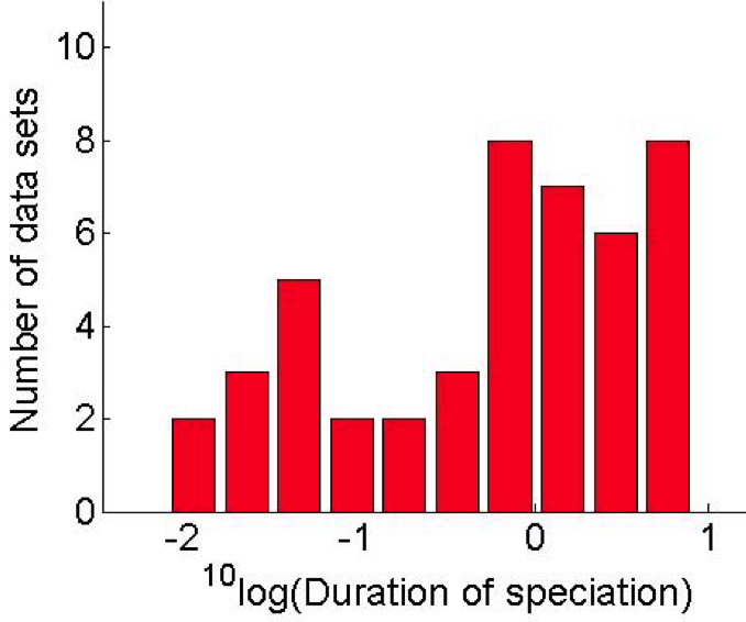
In Etienne et al., (2014) we have developed an inference framework that we tested against 46 bird clades. Individual parameters are difficult to infer, but the method is relatively good at inferring a composite parameter of interest, the duration of speciation. The duration of speciation is defined as the time it takes for a novel population to get a good species in its descendance. The results are shown in Fig 3.7.

3.3.5 Trees with random marks

In this section, trees are endowed with marks to model sampling, detection or mutation.

The phylogeny of pathogens

In this paragraph, we focus on a population of patients carrying (or not) an infectious disease. We stick to the framework of splitting trees, with the interpretation that a birth is a transmission event and a death is either a real death or the end of the infectious period (exit from the infective population). The branching property assumption is justified in the case of a well-mixed population where susceptibles are always in excess.

Our setting where lifetime distributions are not exponential is most attractive for diseases like flu or HIV, where the infectious period is known to be deterministic (flu) or heavy-tailed (HIV).

In addition, we assume that patients are detected to be infective after some random time $D$ , at which they are tagged by a mark (see figures). Upon detection (if $D$ is smaller than the infectious period/lifetime), the patients are assumed to exit the infective population, for example because they change their behaviour to avoid transmission or because they are treated and become non-infectious.

In Lambert et al., 2014a (), we have considered the case where the transmission tree spanned by detected patients has been reconstructed, similarly as Stadler, (2010). Actually, the data is not directly the transmission tree but the phylogenetic tree of the pathogens carried by patients, reconstructed thanks to biological samples taken from the patients upon detection. Fig 3.8 shows the oriented tree of the epidemic, with black dots showing detection events, along with its reduced tree and contour process. Patients can be labelled in the plane order, so we can define $S_{i}$ the detection time of patient $i$ and $R_{i}$ the coalescence time between patients $i-1$ and $i$ .

By considering the jumping contour process of the epidemics, we have shown that the sequence $(S_{i},R_{i})$ is a killed Markov chain. The likelihood of a tree $\mathbbm{t}$ with coalescence times $(x_{i})_{2\leq i\leq n}$ and detection times $(y_{i})_{1\leq i\leq n}$ can be written in the form

\mathscr{L}(\mathbbm{t})=g(y_{1})\,k(y_{n})\,\prod_{i=2}^{n}f(y_{i-1};x_{i},y_{i}),

where $g$ , $k$ and $f$ can be semi-explicitly expressed in terms of the model ingredients (law of infectious lifetimes, transmission rate, detection rate).

Figure 3.8: The transmission tree. a) Binary tree with marks (detection events); b) its reduced tree and c) its contour process.

The state of the epidemics at first detection

We have considered the same setting in Lambert and Trapman, (2013), but for a different question, namely the structure of the epidemic at the first detection time. This question arises in the case of hospital-borne diseases due for example to bacterial antibiotic resistance. In this situation, everything can be known about all carriers of the disease, but only after the first detection of a case. At this random time, denoted $T$ , everybody in the hospital is scanned and infected individuals are identified. Here the phylogeny of pathogens is not assumed to be known but patients’ data like entrance dates or durations of stays are precisely known.

We assume that patients have i.i.d lengths of stay in the hospital, all distributed as some r.v. $K$ . Conditional on infection, the length of stay of a patient is supposed to be a size-biased version of $K$ . Finally, the transmission rate is $b$ and the detection rate per patient is denoted $\delta$ .

For individual $i$ , set

—

$U_{i}:=$ time elapsed from entrance of the hospital up to infection
—

$A_{i}:=$ time elapsed from infection up to $T$
—

$R_{i}:=$ residual lifetime in the hospital after $T$ .

See Fig 3.9 for an example. Set $m:=\mathbb{E}(K)$ and let $\phi$ denote the inverse of the convex function

x\mapsto x-\frac{b}{m}\int_{(0,\infty]}(1-e^{-xy})\,\mathbb{P}(K>y)\,dy.

Figure 3.9: The structure of the stay in the hospital of an infected patient. Some (other) patient is detected at time

T

(random). The focal patient has total duration of stay

K=U+A+R

(see text).

Using Vervaat’s transform applied to the path of the contour process, we were able to show that conditional on $N_{T}=n$ , the triples $(U_{i},A_{i},R_{i})$ of the $n$ infectives at time $T$ are i.i.d. distributed as

\mathbb{E}(f(U,A,R))=\\ \frac{b}{m}\,\frac{\phi(\delta)}{\phi(\delta)-\delta}\ \int_{u=0}^{\infty}du\int_{a=0}^{\infty}da\int_{z=u+a}^{\infty}\mathbb{P}(K\in dz)\,e^{-\phi(\delta)a}\,f(u,a,z-u-a),

In particular, the times $J_{i}=U_{i}+A_{i}$ spent in the hospital up to time $T$ are i.i.d. distributed as the r.v. $J$

\mathbb{P}(J\in dy)=\frac{b/m}{\phi(\delta)-\delta}\ \mathbb{P}(K>y)\,\big(1-e^{-\phi(\delta)y}\big)\,dy.

The last formulae will allow us to infer the dynamical characteristics of hospital-borne disease epidemics from hospital data. This contrasts with the fact that inference is impossible from the sole numbers of cases found upon detection (Trapman and Bootsma, 2009), due to the geometric distribution of $N_{T}$ (recall however that here $T$ is random).

Mutations

Marks on a tree can also be used to model mutations. In population genetics, it is standard to assume that each new mutation occurs at a new site of the DNA sequence, the infinitely-many-sites assumption. The list of mutated sites of a sequence is called allele. One of the fundamental questions in population genetics is to interpret genetic data such as the number of individuals in a population carrying a specific mutation or a specific allele. Reciprocally, the number of mutations, or of alleles, carried by $k$ individuals in the population is called frequency spectrum by sites, or by alleles.

The frequency spectrum of neutral mutations (that is, mutations with no influence on the population dynamics) has been extensively studied for random genealogies arising from models with constant population size, culminating in so-called Ewens’ sampling formula (Ewens, 1972). In a series of recent papers relying heavily on contour techniques, we have studied the frequency spectrum in branching genealogies (Lambert, 2009; Lambert, 2011; Champagnat and Lambert, 2012; Champagnat and Lambert, 2013; Richard, 2014; Delaporte et al., 2016).

3.4 Perspectives

For who has understood how to identify which forward-in-time processes generate trees whose reduced tree is a coalescent point process, and has learnt the procedure of characterizing $W$ and the coalescent density from the model ingredients, coalescent point processes are a very convenient tool:

—

They arise in a wide class of models;
—

They generate robust patterns, that in particular are invariant under incomplete sampling and under the action of bottlenecks;
—

The reconstructed tree has a particularly simple distribution, which is extremely fast to simulate, in contrast with the entire forward-in-time process, that may even not be Markovian;
—

The inference of model parameters from the knowledge of the reconstructed tree can be done using low-tech statistical methods.

On the other hand, CPPs also have a number of shortcomings:

—

The models in which CPP arise exclude some interesting features from the modeling point of view, in particular the trait/age-dependence of birth rates;
—

Among the robust patterns they generate, the shape of the reduced tree is always ERM, which is certainly not the rule in empirical genealogies/phylogenies;

Currently, one of our main lines of research (mine but more generally that of the SMILE group – Stochastic models for the inference of life evolution, UPMC & Collège de France) is to produce and study models that

1.

are grounded on the microscopic description of individuals, either at the ecological scale or at the genetic scale;
2.

feature a small number of parameters, which can nevertheless be tuned so as to generate a wide range of different patterns, when the corresponding empirical patterns vary across datasets (e.g., species abundance distributions);
3.

generate robust patterns when the corresponding empirical patterns are well conserved across datasets (e.g., the MLE of $\beta$ in empirical phylogenies, that revolves around $-1$ );
4.

produce observable statistics (e.g., reconstructed trees) with computable likelihoods.

Criterion 3 is in general difficult to satisfy, especially simultaneously with 2.

References

Aldous, (1991) Aldous, D. (1991). The Continuum Random Tree. I. The Annals of Probability, 19(1):1–28.
Aldous, (1993) Aldous, D. (1993). The Continuum Random Tree III. The Annals of Probability, 21(1):248–289.
Aldous, (1996) Aldous, D. (1996). Probability Distributions on Cladograms. In Friedman, A., Miller, W., Aldous, D., and Pemantle, R., editors, Random Discrete Structures, volume 76, pages 1–18. Springer New York, New York, NY.
Aldous and Popovic, (2005) Aldous, D. and Popovic, L. (2005). A critical branching process model for biodiversity. Advances in Applied Probability, 37(4):1094–1115.
Aldous, (2001) Aldous, D. J. (2001). Stochastic models and descriptive statistics for phylogenetic trees, from Yule to today. Statistical Science, 16(1):23–34.
Barthélémy and Guénoche, (1991) Barthélémy, J.-P. and Guénoche, A. (1991). Trees and Proximity Representations. John Wiley & Sons.
Bertoin, (1996) Bertoin, J. (1996). Lévy processes, volume 121 of Cambridge Tracts in Mathematics. Cambridge University Press, Cambridge.
Bertoin, (2006) Bertoin, J. (2006). Random fragmentation and coagulation processes, volume 102 of Cambridge Studies in Advanced Mathematics. Cambridge University Press, Cambridge.
Blum and François, (2006) Blum, M. G. and François, O. (2006). Which random processes describe the tree of life? A large-scale study of phylogenetic tree imbalance. Systematic Biology, 55(4):685–691.
Brown, (1994) Brown, J. K. M. (1994). Probabilities of evolutionary trees. Systematic Biology, 43(1):78–91.
Burago et al., (2001) Burago, D., Burago, Y., and Ivanov, S. (2001). A Course in Metric Geometry, volume 33. American Mathematical Society Providence.
Champagnat and Lambert, (2012) Champagnat, N. and Lambert, A. (2012). Splitting trees with neutral Poissonian mutations I: Small families. Stochastic Processes and their Applications, 122(3):1003–1033.
Champagnat and Lambert, (2013) Champagnat, N. and Lambert, A. (2013). Splitting trees with neutral Poissonian mutations II: Largest and oldest families. Stochastic Processes and their Applications, 123(4):1368–1414.
Delaporte et al., (2016) Delaporte, C., Achaz, G., and Lambert, A. (2016). Mutational pattern of a sample from a critical branching population. Journal of Mathematical Biology, pages 1–38.
Dress et al., (1996) Dress, A., Moulton, V., and Terhalle, W. (1996). T-theory: An overview. European Journal of Combinatorics, 17(2–3):161–175.
Duquesne, (2006) Duquesne, T. (2006). The coding of compact real trees by real valued functions. arXiv:math/0604106. arXiv: math/0604106.
Duquesne and Le Gall, (2002) Duquesne, T. and Le Gall, J.-F. (2002). Random trees, Lévy processes and spatial branching processes, volume 281. Société mathématique de France.
Etienne et al., (2014) Etienne, R. S., Morlon, H., and Lambert, A. (2014). Estimating the duration of speciation from phylogenies. Evolution, 68(8):2430–2440.
Etienne and Rosindell, (2012) Etienne, R. S. and Rosindell, J. (2012). Prolonging the past counteracts the pull of the present: protracted speciation can explain observed slowdowns in diversification. Systematic Biology, 61(2):204–213.
Evans, (2008) Evans, S. N. (2008). Probability and Real Trees: École d’été de Probabilités de Saint-Flour XXXV-2005. Springer.
Evans et al., (2005) Evans, S. N., Pitman, J., and Winter, A. (2005). Rayleigh processes, real trees, and root growth with re-grafting. Probability Theory and Related Fields, 134(1):81–126.
Ewens, (1972) Ewens, W. J. (1972). The sampling theory of selectively neutral alleles. Theoretical Population Biology, 3:87–112; erratum, ibid. 3 (1972), 240; erratum, ibid. 3 (1972), 376.
Geiger, (1996) Geiger, J. (1996). Size-biased and conditioned random splitting trees. Stochastic Processes and their Applications, 65(2):187–207.
Geiger and Kersting, (1997) Geiger, J. and Kersting, G. (1997). Depth-first search of random trees, and Poisson point processes. In Classical and modern branching processes (Minneapolis, MN, 1994), volume 84 of IMA Vol. Math. Appl., pages 111–126. Springer, New York.
Haas, (2016) Haas, B. (2016). Scaling limits of Markov-Branching trees and applications. Eprint arXiv:1605.07873.
Haas et al., (2008) Haas, B., Miermont, G., Pitman, J., and Winkel, M. (2008). Continuum tree asymptotics of discrete fragmentations and applications to phylogenetic models. The Annals of Probability, 36(5):1790–1837.
Hagen et al., (2015) Hagen, O., Hartmann, K., Steel, M., and Stadler, T. (2015). Age-dependent speciation can explain the shape of empirical phylogenies. Systematic Biology, 64(3):432–440.
Harding, (1971) Harding, E. F. (1971). The probabilities of rooted tree-shapes generated by random bifurcation. Advances in Applied Probability, 3(1):44–77.
Jetz et al., (2012) Jetz, W., Thomas, G. H., Joy, J. B., Hartmann, K., and Mooers, A. O. (2012). The global diversity of birds in space and time. Nature, 491(7424):444–448.
Kingman, (1982) Kingman, J. (1982). The coalescent. Stochastic processes and their applications, 13(3):235–248.
Knuth, (1997) Knuth, D. E. (1997). The Art of Computer Programming. Addison-Wesley.
Kyprianou, (2006) Kyprianou, A. E. (2006). Introductory lectures on fluctuations of Lévy processes with applications. Universitext. Springer-Verlag, Berlin.
Lambert, (2008) Lambert, A. (2008). Population Dynamics and Random Genealogies. Stochastic Models, 24(suppl. 1):45–163.
Lambert, (2009) Lambert, A. (2009). The allelic partition for coalescent point processes. Markov Processes and Related Fields, 15(3):359–386.
Lambert, (2010) Lambert, A. (2010). The contour of splitting trees is a Lévy process. The Annals of Probability, 38(1):348–395.
Lambert, (2011) Lambert, A. (2011). Species abundance distributions in neutral models with immigration or mutation and general lifetimes. Journal of Mathematical Biology, 63(1):57–72.
(37) Lambert, A., Alexander, H. K., and Stadler, T. (2014a). Phylogenetic analysis accounting for age-dependent death and sampling with applications to epidemics. Journal of Theoretical Biology, 352:60–70.
(38) Lambert, A., Morlon, H., and Etienne, R. S. (2014b). The reconstructed tree in the lineage-based model of protracted speciation. Journal of Mathematical Biology, 70(1-2):367–397.
Lambert and Popovic, (2013) Lambert, A. and Popovic, L. (2013). The coalescent point process of branching trees. Annals of Applied Probability, 23(1):99–144.
Lambert et al., (2013) Lambert, A., Simatos, F., and Zwart, B. (2013). Scaling limits via excursion theory: Interplay between Crump-Mode-Jagers branching processes and Processor-Sharing queues. The Annals of Applied Probability, 23(6):2357–2381.
Lambert and Stadler, (2013) Lambert, A. and Stadler, T. (2013). Birth–death models and coalescent point processes: The shape and probability of reconstructed phylogenies. Theoretical Population Biology, 90:113–128.
Lambert and Steel, (2013) Lambert, A. and Steel, M. (2013). Predicting the loss of phylogenetic diversity under non-stationary diversification models. Journal of Theoretical Biology, 337:111–124.
Lambert and Trapman, (2013) Lambert, A. and Trapman, P. (2013). Splitting trees stopped when the first clock rings and Vervaat’s transformation. Journal of Applied Probability, 50(1):208–227.
(44) Lambert, A. and Uribe Bravo, G. (2016a). The comb representation of compact ultrametric spaces. Eprint arXiv:1602.08246.
(45) Lambert, A. and Uribe Bravo, G. (2016b). Totally ordered, measured trees and splitting trees with infinite variation. Eprint arXiv:1607.02114.
Le Gall, (1993) Le Gall, J.-F. (1993). The uniform random tree in a Brownian excursion. Probability Theory and Related Fields, 96(3):369–383.
Le Gall, (2005) Le Gall, J.-F. (2005). Random trees and applications. Probability Surveys, Vol. 2, 2005.
Le Gall and Miermont, (2012) Le Gall, J.-F. and Miermont, G. (2012). Scaling limits of random trees and planar maps. In Ellwood, D., editor, Probability and Statistical Physics in Two and More Dimensions: Proceedings of the Clay Mathematics Institute Summer School and XIV Brazilian School of Probability, 2010. American Mathematical Society.
Manceau et al., (2015) Manceau, M., Lambert, A., and Morlon, H. (2015). Phylogenies support out-of-equilibrium models of biodiversity. Ecology Letters, 18(4):347–356.
Mooers et al., (2012) Mooers, A., Gascuel, O., Stadler, T., Li, H., and Steel, M. (2012). Branch lengths on birth–death trees and the expected loss of phylogenetic diversity. Systematic Biology, 61(2):195–203.
Murtagh, (1984) Murtagh, F. (1984). Counting dendrograms: A survey. Discrete Applied Mathematics, 7(2):191–199.
Nee, (2006) Nee, S. (2006). Birth-death models in macroevolution. Annual Review of Ecology, Evolution and Systematics, 37:1–17.
Nee et al., (1994) Nee, S., May, R., and Harvey, P. (1994). The reconstructed evolutionary process. Philosophical Transactions of the Royal Society of London. Series B: Biological Sciences, 344(1309):305–311.
Nee and May, (1997) Nee, S. and May, R. M. (1997). Extinction and the loss of evolutionary history. Science, 278(5338):692–694.
Paulin, (1989) Paulin, F. (1989). The Gromov topology on $R$ -trees. Topology and its Applications, 32(3):197–221.
Pitman, (2006) Pitman, J. (2006). Combinatorial Stochastic Processes: École d’été de Probabilités de Saint-Flour XXXII - 2002. Springer.
Popovic, (2004) Popovic, L. (2004). Asymptotic genealogy of a critical branching process. Annals of Applied Probability, pages 2120–2148.
Richard, (2014) Richard, M. (2014). Splitting trees with neutral mutations at birth. Stochastic Processes and their Applications, 124(10):3206 – 3230.
Semple and Steel, (2003) Semple, C. and Steel, M. A. (2003). Phylogenetics, volume 24. Oxford University Press.
Slowinski, (1990) Slowinski, J. B. (1990). Probabilities of $n$ -trees under two models: a demonstration that asymmetrical interior nodes are not improbable. Systematic Biology, 39(1):89–94.
Stadler, (2010) Stadler, T. (2010). Sampling-through-time in birth–death trees. Journal of Theoretical Biology, 267(3):396–404.
Stadler, (2011) Stadler, T. (2011). Mammalian phylogeny reveals recent diversification rate shifts. Proceedings of the National Academy of Sciences, 108(15):6187–6192.
Stanley, (1999) Stanley, R. P. (1999). Enumerative Combinatorics. Vol. 2, volume 62 of Cambridge Studies in Advanced Mathematics. Cambridge University Press, Cambridge.
Trapman and Bootsma, (2009) Trapman, P. and Bootsma, M. C. J. (2009). A useful relationship between epidemiology and queueing theory: The distribution of the number of infectives at the moment of the first detection. Mathematical Biosciences, 219(1):15–22.

	$\displaystyle\|d_{1}(x_{1},y_{1})-d_{2}(x_{2},y_{2})\|$	$\displaystyle\leq$	$\displaystyle\|h_{1}\circ\lambda-h_{2}\|(s)+\|h_{1}\circ\lambda-h_{2}\|(t)+2\,\|\inf_{[s,t]}h_{1}\circ\lambda-\inf_{[s,t]}h_{2}\|$
		$\displaystyle\leq$	$\displaystyle 4\\|h_{1}\circ\lambda-h_{2}\\|.$

Abstract:

Keywords:

Chapter 1 Tree shapes

1.1 Definitions

Exercise 1.1.1.

1.2 Combinatorics warm up

1.2.1 Counting trees

Definition 1.2.1.

Definition 1.2.2.

Example 1.2.3.

Definition 1.2.4.

Proposition 1.2.5 (Murtagh, 1984).

Remark 1.2.6.

Proof.

Exercise 1.2.7.

Exercise 1.2.8.

1.2.2 Counting rankings and labellings

Definition 1.2.9.

Definition 1.2.10.

Exercise 1.2.11.

Definition 1.2.12.

Proposition 1.2.13 (Knuth, 1997).

Proof.

1.3 Random tree shapes

1.3.1 Uniform distributions

Definition 1.3.1.

Remark 1.3.2.

Exercise 1.3.3.

1.3.2 The law of your favourite random tree

The Bienaymé–Galton–Watson tree shape

Proposition 1.3.4.

The Yule tree shape

Proposition 1.3.5.

Proof.

The Kingman tree shape

Proposition 1.3.6.

Proof.

Exercise 1.3.7.

1.4 Markov branching models

1.4.1 Definitions and interval splitting

Definition 1.4.1 (Aldous, 1996).

Remark 1.4.2.

Exercise 1.4.3.

1.4.2 ERM, PDA and Aldous’ β\beta-splitting model

Theorem 1.4.4 (Harding, 1971; Slowinski, 1990; Brown, 1994).

Proof.

Exercise 1.4.5.

Back to the Galton–Watson tree

Aldous’ β\beta-splitting model

Exercise 1.4.6.

Remark 1.4.7.

Proposition 1.4.8.

Proof.

Exercise 1.4.9.

1.4.3 Sampling consistency

Exercise 1.4.10.

Theorem 1.4.11.

Remark 1.4.12.

Remark 1.4.13.

Proof of Theorem 1.4.11.

Chapter 2 Real Trees

2.1 Preliminaries

2.1.1 Scaling limits

2.1.2 Local time

2.2 Definitions and examples

2.2.1 The real tree

Definition 2.2.1.

Theorem 2.2.2 (Four points condition).

Definition 2.2.3.

Exercise 2.2.4.

2.2.2 First constructive example: Connecting segments

2.2.3 Second constructive example: Chronological trees

Definition 2.2.5.

Definition 2.2.6.

Exercise 2.2.7.

Theorem 2.2.8.

Exercise 2.2.9.

Remark 2.2.10.

2.3 The contour process

2.3.1 From the ℝ\mathbb{R}-tree to its contour process

1.4.2 ERM, PDA and Aldous’ $\beta$ -splitting model

Aldous’ $\beta$ -splitting model

2.3.1 From the $\mathbb{R}$ -tree to its contour process

2.4 Random $\mathbb{R}$ -trees

3.1.2 Spheres of $\mathbb{R}$ -trees