Inference of Internal Stress in a Cell Monolayer
V. Nier1, S. Jain2, C. T. Lim2,3, S. Ishihara4, B. Ladoux2,5 and P. Marcq1,*
1 Sorbonne Universités, UPMC Univ Paris 6,
Institut Curie, CNRS, UMR 168, Laboratoire Physco-Chimie Curie, Paris, France
2 Mechanobiology Institute, National University of Singapore,
Singapore
3 Department of Biomedical Engineering and Department of
Mechanical Engineering, National University of Singapore, Singapore
4 Department of Physics, Meiji University, Kawasaki,
Kanagawa, Japan
5 Institut Jacques Monod, CNRS UMR 7592 and Université Paris
Diderot, Paris, France
* Corresponding Author philippe.marcq@curie.fr
Abstract
We combine traction force data with Bayesian inversion to obtain an absolute estimate of the internal stress field of a cell monolayer. The method, Bayesian inversion stress microscopy (BISM), is validated using numerical simulations performed in a wide range of conditions. It is robust to changes in each ingredient of the underlying statistical model. Importantly, its accuracy does not depend on the rheology of the tissue. We apply BISM to experimental traction force data measured in a narrow ring of cohesive epithelial cells, and check that the inferred stress field coincides with that obtained by direct spatial integration of the traction force data in this quasi-one-dimensional geometry.
1 Introduction
Dynamical behaviors of multicellular assemblies play a crucial role during tissue development [1] and in the maintenance of adult tissues [2]. In addition, disregulation of multicellular structures may lead to pathological situations such as tumor formation and tumor progression [3]. In this context, cell monolayers have been extensively studied to model in vivo tissue functions. Such approaches allow for well-controlled experiments, which have been performed in a variety of settings, such as monolayer spreading [4, 5], wound healing [6, 7], channel flow [8, 9], confined flow [10, 11], collective migration [12, 13]. The dynamics of multicellular assemblies is regulated through mechanical forces that act upon cell adhesive structures. These forces are exerted at the cell-substrate interface [14], but also through cell-cell junctions [15]. The transmission of stresses within multicellular assemblies is thus important to understand collective movements, cell rearrangements and tissue homeostasis. Even though kinematic information is readily available, mechanical properties that rely on internal stress are less well understood. Indeed a number of important biological questions, such as the determination of the molecular mechanisms that underlie the transmission of force within a tissue [16], necessitate a measurement of internal stresses.
Several internal force measurement methods have been proposed and implemented (see [17] for a recent review): at the molecular scale, Förster resonance energy transfer [18, 19]; at the cell scale, microrheology [20, 21]; at the tissue scale, liquid drops [22], birefringence [23], or laser ablation [24, 25]. Although one would ideally like to read out from data the spatio-temporal dependence of the full stress field, the above methods yield either a local, sub-tissue scale measurement [18, 19, 20, 21, 22]; or a subset of the components of the stress tensor [23], or a relative measurement, up to an undetermined multiplicative constant [24, 25]. Monolayer stress microscopy (MSM), first introduced in [26], does not suffer from these drawbacks: it builds upon the measurement of traction force data to estimate the stress field of monolayers of cohesive cells. Indeed, the force exerted by cells on a planar deformable substrate can be computed from the displacement field of the underlying layer [27, 28], using either: (i) traction force microscopy [29, 30, 5] where small beads are inserted within the (elastic) substrate, their displacements are measured, and the traction forces are obtained by solving an inverse elastic problem; or (ii) arrays of micropillars [31, 32, 33], where the traction forces are simply proportional to the in-plane displacements of the pillars. However, once the traction forces are known, obtaining the internal stress from the force balance equations is an underdetermined problem since, in the two dimensional case, three components of the symmetrical stress tensor must be obtained from two traction force components. In MSM [26, 34], these equations become well-posed thanks to an additional hypothesis on tissue rheology: the cell monolayer is assumed to be a linear, isotropic elastic body. MSM has been validated independently on numerical data using particle dynamics simulations: in [35], the reasonable accuracy of stress reconstruction from data that does not correspond to an elastic rheology has been attributed to the weakness of shear stresses in both simulated and living tissues. Assuming again that the tissue is an elastic body, and in addition that the displacement field is continuous at the cell-substrate interface, internal stresses may also be computed directly from substrate displacement data, circumventing the need to compute traction forces [36].
In the presence of cell divisions and extrusions that constantly rearrange a tissue [37], it is not clear that its rheology is that of a solid body. To our knowledge, the elastic rheology hypothesis has not been directly validated, while alternative rheologies have been proposed in the literature [38, 39, 40, 7] and shown to model successfully specific aspects of the mechanical behaviour of cell monolayers. Further, the rheology of multicellular assemblies may depend on the timescale [37], as well as on the type of cell considered [41]. These caveats call for a method to accurately estimate the internal stress field of a cell monolayer irrespective of the underlying rheology.
A classical way to solve underdetermined inversion problems involves Bayesian inference [42], a technique originating in statistics [43], and now widely used in physics [44] and biophysics [45]. Of note, Bayesian inversion has also been used to solve the inverse elastic problem of traction force microscopy [46, 47]. Recently, some among us proposed a Bayesian force inference method based on cell geometry, and applied it to segmented images of the Drosophila pupal wing and notum [48, 49, 50]. The tissue-scale stress arises from coarse-graining of cell-cell interactions. For tight epithelia where adherens junctions are a key player of force transmission between neighboring cells, it is reasonable to assume that the cell-scale contribution to stress is mostly related to local contact within the apical side of the epithelium, whereas basal contributions from, e.g. lamellipodia, are negligible. Accordingly, the dominant contributors to tissue-scale stress were identified as cell pressures and cell-cell junction tensions, and force balance equations were written at each cell vertex, resulting in an underdetermined system. This system was solved using Bayesian inversion [42], where the inferred tensions and pressures were the most likely values (the modes) of a posterior distribution function. In the case of the fruitfly pupal wing, it turned out that tissue stress, obtained by coarse-graining, is oriented by external forces, and that its anisotropy promotes hexagonal cell packing [49]. Similar systems of equations may become well-posed thanks to additional hypotheses (equal cell pressures [50, 51]), or when cell pressures are not required [52]. However the stress is measured up to an arbitrary additive constant: its absolute value is out of reach since the input data are cell vertex positions and cell junction angles.
Below, we formulate Bayesian inversion stress microscopy (BISM), a method to estimate the internal stress field of a cell monolayer from traction force microscopy measurements. Importantly, BISM yields an absolute measure of the stress and dispenses with hypotheses on monolayer rheology. We define BISM and introduce statistical measures of its accuracy. The method is first validated using numerical simulations that provide traction force data. The inferred stress field, once computed, is compared to the simulated stress data used as a reference. Robustness is checked by implementing changes in the statistical model, as well as in the mechanical ingredients of the numerical simulations. BISM is further validated using experimental data in a quasi-one-dimensional geometry that allows for a direct calculation of the stress field by spatial integration of the traction force field. Finally, our results are compared with existing methods.
2 Methods
2.1 Mechanics
Within a continuum description, a flat, thin cell monolayer is characterized at position and time by a field of two-dimensional internal stresses and by a field of external surfacic forces that the monolayer exerts on the substrate. Since inertia is negligible, the balance of linear momentum reads in vector form
| (1) |
and in cartesian coordinates (see Supplementary Text 1.2 for polar coordinates)
| (2) | |||||
| (3) |
Note that at this stage, due to the grid definition (see below and Fig. 1b), we do not enforce the symmetry of the stress tensor (equality of the shear stress components due to angular momentum conservation [53]). With a confined monolayer in mind [10, 11], the boundary condition reads
| (4) |
where denotes the vector normal to the edge, and summation over repeated indices is implied. In the plane, the units of stresses and (surfacic) forces are Pa.m and Pa respectively. Assuming that the monolayer height is uniform and constant , the 3D stress reads . When spatial or temporal variations of the height cannot be neglected [4, 5], BISM can be implemented by replacing by and by inferring the 3D stress from , provided that the height remains small compared to the system size, as is generally the case for in vitro cell monolayers [26, 54]. A treatment of the full 3D case where the height is comparable or larger than the system size is beyond the scope of this work.

Since experimental traction forces are measured with a finite spatial resolution , assumed to be isotropic for simplicity, we write a force balance equation in each of a large number of square surface elements of area (see Fig. 1a). We aim at inferring the stress tensor in each element. The traction force exerted by the tissue in element on the substrate is , with components . In the case of a rectangular grid with columns and rows, the discretized force balance equation for element reads
| (5) | |||||
| (6) |
to lowest order in (see Fig. 1b). We thus have variables for and , variables for and and variables for and . Defining traction force and stress vectors as
where the superscript t denotes the transpose, we rewrite Eqs. (5-6) in matrix form
| (7) |
The matrix , of size , may be decomposed as
| (8) |
where and correspond to the discretized matrix forms, at second order in , of the partial derivatives with respect to and .
2.2 Statistics
To solve the underdetermined linear system (7), we implement Bayesian inversion [42]: all variables and parameters of the problem are probabilized. For simplicity, we use wherever possible Gaussian probability distribution functions, denoted for a multivariate (vector) Gaussian random variable with mean and covariance matrix .
Likelihood
The first ingredient of the statistical model is the likelihood function , which contains information provided by experimental measurements. For experimental data, the force balance equations (7) are verified up to an additive noise due to measurement errors. Assuming this noise to be Gaussian with zero mean and uniform covariance matrix , where the parameter denotes the noise variance and is the identity matrix, the likelihood is expressed as or
| (9) |
where is the (L2) Euclidean norm.
Prior
Second, the prior probability distribution function embeds additional information concerning the stress field:
- (i)
we assume that the stress obeys a Gaussian distribution function with zero mean and covariance matrix ;
- (ii)
we enforce the equality of the two off-diagonal components of the stress tensor: in compact vector form , i.e. (see Fig. 1b and ST 1.3);
- (iii)
we enforce the boundary conditions (4), namely two conditions at each boundary element , written in compact vector form ).
Up to a normalizing factor, the prior reads
| (10) |
or
| (11) |
The second ingredient of the statistical model is a Gaussian prior where is a reduced covariance matrix of determinant . Note that a Gaussian prior suppresses stress values larger than a few times (see [55] for a similar approach in the context of traction force microscopy). In practice, we set the hyperparameters and to the values , large enough for conditions (ii) and (iii) to be enforced (see ST 3.2 for a discussion of these values). If required by a given experimental set-up, the boundary conditions should be modified appropriately in the definition of the prior.
Resolution
According to Bayes’ theorem, the posterior (conditional) probability distribution function of the stress given the traction force data is proportional to the product of the likelihood by the prior
| (12) |
Since both are Gaussian, the posterior is also Gaussian , with a covariance matrix and a mean given by [42]
| (13) | |||||
| (14) |
We use maximum a posteriori (MAP) estimation [42] and define the inferred stress as the mode (maximal value) of the posterior . Qualitatively, the underdeterminacy has been lifted: unknown stress values are determined from traction force values, conditions from the Gaussian distribution of the stress tensor, equalities of the two shear components and boundary conditions.
In this Gaussian model, MAP estimation is identical to minimization of a Tikhonov potential [42]. The dimensionless regularization parameter
| (15) |
quantifies the relative weight given to the prior, compared to the likelihood, when performing Bayesian inversion. Factoring out , Eqs. (13-14) read
| (16) | |||||
| (17) |
Since the product is dimensionless and independent of , the posterior covariance (16) is a function of and , while the posterior mode (17) depends upon and .

Hyperprior
For generality sake, we probabilize the parameter and the hyperparameter , yet undetermined in Eqs. (13-14) (recall that and ). Within the framework of hierarchical Bayesian descriptions, the model is closed by the hyperprior probability distribution functions and [56, 57]. Up to a normalizing factor, the posterior now reads (see Fig. 2a)
| (18) |
For simplicity, we use Jeffreys’ non-informative hyperprior: , [56, 57].
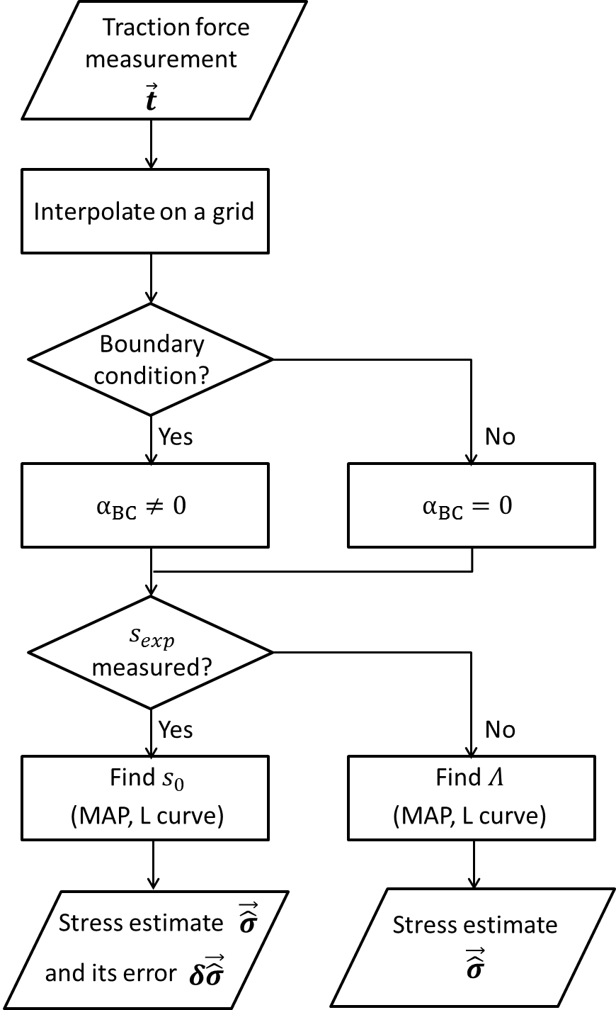
Simultaneous a posteriori optimization with respect to , and being intractable, we solve the problem iteratively, starting from initial values and (see Fig. 2b). At step , we first calculate the mode from previous values , , Eqs. (13-14). Maximizing the posterior with respect to each hyperparameter yields the updated hyperparameter values
| (19) | |||||
| (20) |
Once convergence is reached, , , the stress estimate is defined as , computed from Eqs. (13-14) with the optimal values and . An estimate of the error on is calculated as the square root of the diagonal values of the covariance matrix . Since the marginal distribution of traction forces is Gaussian, with a covariance matrix [42], we also calculate an estimate of the error on the traction force as the square root of the diagonal values of .
2.3 Measures of accuracy
The numerical resolution of a set of hydrodynamical equations yields a numerical data set of traction forces, from which we compute a set of inferred stresses. Since the numerical data set of stresses is also available, measures of accuracy involving numerical simulations typically compare with .
A classical “goodness-of-fit” measure is the coefficient of determination, defined for the component of the stress as
| (21) |
where the sums and the averages are performed over space. Similar definitions apply to other components, and allow to define an aggregate coefficient of determination averaged over all stress components. Accurate estimates correspond to numerical values of close to . The discretized force balance equations (5-6), used as a definition of inferred traction forces, yield a set of inferred traction forces computed from the set of inferred stresses . Comparing with allows to define similarly a diagnostic for numerical data.
When analyzing an experimental data set of traction forces, cannot be computed in the absence of a reference set of stresses. As above, comparing with allows to define a measure of accuracy for experimental data, the coefficient of determination . An alternative measure of predictive accuracy is the diagnostic, defined as the average value of the square of reduced residuals
| (22) |
where the sum is performed over space and over traction force components. This measure of accuracy is, up to a normalizing factor, similar to the “omnibus goodness-of-fit” measure advocated in [56, 57]. The estimated standard deviation may be replaced in Eq. (22) by the measurement error . Numerical values of close to are indicators of high accuracy.
2.4 Experimental methods
We used MDCK (Madin-Darby canine kidney) cells as an epithelial cell model.
Cell Culture
MDCK wild-type cells were cultured in media containing DMEM (Life Technologies), FBS (Life Technologies) and antibiotics (penicillin and streptomycin).
Micro-contact printing and substrate preparation for Traction Force Microscopy
We measured the traction forces exerted by cells on their substrate by using soft silicone gel as previously described [58]. Fluorescent beads were deposited onto the gel to measure the displacement field. Briefly, a thin layer of the gel was spread on a glass bottom dish and then cured at C for hours. Cured gel was silanized using solution of (3-aminopropyl) triethoxysilane (APTES, Sigma) in pure ethanol. This gel was later incubated for minutes with nm carboxylated fluorescent beads (Invitrogen) suspended in deionized (DI) water. Subsequently, the substrate was dried and micro-contact printed with fibronectin [13, 59] using a thin water soluble Polyvinyl Alcohol (PVA) membrane which allows the transfer of fibronectin on soft gel. The PVA membrane was later dissolved and the non-contact printed areas were blocked using pluronics (Sigma) solution. The substrate was then washed and was seeded with cells. Cells were allowed to grow until the micro-contact printed area was fully covered.
The images were acquired using phase contrast and fluorescent channels to record cell positions and bead displacements, respectively.
For analysis, the imaging drifts were corrected in ImageJ (NIH) using the Image Stabilizer plugin [60]. To analyze the displacement field of beads, we used an open source iterative PIV (particle image velocimetry) plugin in ImageJ [61]. To reconstruct the traction force field from the obtained displacement field, an open source Fourier transform traction cytometry (FTTC) plugin was used in ImageJ [61]. The resulting traction force values were taken for the validation of the BISM inferred stress fields. To estimate the experimental error made on traction force measurements, we calculated the mean value of traction forces measured on square regions of the substrate devoid of cells (surface area ).
Monolayer height measurement
The confluent cell monolayer was fixed for immunofluorescence microscopy. Actin present inside the cells was fluorescently labeled using Alexa Fluor 488-conjugated phalloidin (Invitrogen) at 1:1000 dilution in PBS. To measure tissue height, overall cell shape was then visualized with the help of cortical actin. Imaging was done using a Zeiss LSM 780 confocal microscope with a step size of to capture the entire height of the tissue. In the confined ring shape geometry, height was measured at different locations to obtain the mean value and standard deviation of the monolayer height m.
3 Results
3.1 Validation: numerical data
A first example of the application of BISM to a numerical data set is given by using the traction force field of a compressible viscous fluid driven by active force dipoles, interacting with its substrate through an effective fluid friction force, and confined in a square, with the boundary conditions (4). We solve this problem on a square over a regular cartesian grid with , and (see ST 1.1). We use material parameter values typical of cell monolayers: friction coefficient [7], shear viscosity [62], and compression viscosity . To account for the measurement error, we add to the traction force field a white noise of relative amplitude (variance ), and obtain the numerical data set of traction forces (Fig. 3a), referred to below as Viscous. We checked that the total sum of the traction forces is close to zero, as expected for a closed system with negligible inertia.

Bayesian inversion is performed with a custom-made script written in Matlab (The MathWorks, Inc.). With and as initial values, the resolution method converges in a few steps towards the asymptotic hyperparameter values and , or (see ST 3.1 and Fig. S4a in the Supporting Material) The data sets and of simulated and inferred stresses are shown in Fig. 3b-c: we find that their spatial structures are quite similar. This observation is confirmed quantitatively by plotting component by component the inferred stress vs. the simulated stress (Figs. 3d-f), and by the numerical values of the coefficients of determination , , , yielding an aggregate measure of accuracy , close to . Using the inferred data set of traction forces, we also obtain and , indicating that all the information contained in the traction force data is used. An order of magnitude of the error bar is given by the standard deviations, calculated using (16): , corresponding to of the maximal stresses.
All qualitative and quantitative indicators show that the stress field has been inferred accurately.
3.2 Robustness to variations of the statistical model
We test the robustness of BISM by varying one by one each feature of the statistical model, first focusing on alternative definitions of the prior, arguably our most prominent assumption, second modifying the likelihood, the hyperprior and the resolution method. For conciseness, precise definitions and implementations are given in ST 2.1-2.3. Table S1 in the Supporting Material lists the values of thus obtained, given the same numerical data sets as for BISM.
Setting to in the definition of the prior has a significant influence on the accuracy of inference (): the symmetry of the stress tensor needs to be enforced in the prior for accurate estimation. Unsurprisingly, this impacts less the diagonal () than the shear components (). In a similar way, knowledge of the correct boundary conditions should be included in the prior whenever possible: setting to has a large negative impact ). We shall further comment below on the influence of boundary conditions.
Importantly, the accuracy of inference remains excellent when the prior, the likelihood, or the hyperprior distributions are not Gaussian. This shows that the accuracy of BISM does not depend sensitively on a Gaussian assumption. Of note, we do not assume that traction force data obeys a Gaussian distribution. The data set ( or ) is used as is – indeed experimental traction force distributions are known to exhibit exponential tails [5, 63]. In all cases, the regularization parameter is small (see Table S3 in the Supporting Material): the distribution of inferred stresses depends mostly on the empirical distribution of traction force data. Thus, even if the multivariate posterior distribution is Gaussian, the univariate, empirical distribution of the inferred stress (the mode ) is not necessarily Gaussian (see Fig. S7 in the Supporting Material for numerical data). Similarly, even if the stress prior distribution function has a zero mean, the mean inferred stress is not necessarily equal to zero (see Fig. 5i for an example). The small values of are consistent with robustness with respect to variations of the prior.
We conclude that BISM is robust to variations of the statistical model.

3.3 Robustness to variations of the numerical simulation
We next apply BISM to a broad spectrum of numerical data, and vary successively the values of material parameters, the rheology, the boundary conditions, the system shape, the spatial resolution, the nature and the amplitude of the measurement noise (see ST 2.2).
Given the values of compiled in Table S2 in the Supporting Material, we verify that BISM remains accurate with a different (elastic) rheology (also set Elastic 1 in Table 1), or in a different (circular) geometry. In the viscous case, we observe that the accuracy decreases as a function of the bulk viscosity . For larger , we observe larger values of stress components, leading to asymmetrical distributions: this is at variance with our assumption of an even prior distribution, and may explain the lower value of obtained when .
Accuracy decreases when the prior does not include our knowledge of the boundary conditions. However the influence of erroneous values of the stress at the system’s boundaries rapidly decreases far from the edge. When the coefficient is set to , removing the outtermost rows and columns increases from to . We estimate the corresponding “penetration length” of boundary values to about of the system size, consistent with [34]. We conclude that, whenever available, the correct boundary conditions should be taken into account in the prior.
Importantly (see Fig. 4), accuracy remains acceptable () for a spatial resolution larger than a few data points per cell, as well as for measurement noise levels up to of the traction force amplitude, consistent with measurement errors typical of force traction microscopy [31].
These results highlight that BISM is robust to variations of the numerical simulations that yield the traction force data.
3.4 Validation: experimental data
While inverting the force balance equations (1) requires specific techniques in 2D, the same problem reduces in 1D to straightforward integration along the spatial coordinate [5]. For this reason, we fabricated a micro-patterned ring whose measured mean radius is larger than its width , measured the substrate displacement field, and deduced the traction forces exerted by a monolayer of MDCK cells confined within the ring (Figs. 5a-c, see Experimental Methods for further details). We find an average traction force amplitude Pa for a measurement error of the order of Pa, and deduce a relative error of the order of , consistent with the range of noise amplitudes where BISM was deemed applicable, see Fig. 4. The height of the monolayer is typically m (see Sec. 2.4), much smaller than the spatial extension , and varies smoothly, see Fig. S8 in the Supporting Material. In Figs. 5d-f, we plot the three stress components as inferred by BISM, with a regularization parameter and a traction force-based measure of accuracy , as defined by Eq. (22). Note that the inferred stresses are mostly positive, even though the prior distribution is a zero-mean Gaussian, see Fig. 5i.

Since shear stresses are small compared to angular normal stresses , the orthoradial component of the force balance equation (see ST 1.2) simplifies to
| (23) |
Taking into account the experimental angular resolution , and averaging radially over the width of the ring, we obtain the 1D value of the increment of orthoradial stress over :
| (24) |
This value is compared with the radially-averaged increment of orthoradial stress inferred by BISM (Figs. 5g-h). The excellent agreement found between experimental () and inferred () 1D stresses is quantified by a coefficient of determination , see Fig. 5h. To check that BISM allows to infer absolute stress values, we calculate the average pressure from traction force data (see ST 1.4):
| (25) |
where denotes spatial averaging over the whole domain. We obtain , in agreement with the average inferred pressure .
We conclude that BISM is readily applicable to experimental traction force data, and has been validated on experimental data without reference to a specific rheological model of the tissue.
3.5 Comparison with monolayer stress microscopy
Monolayer stress microscopy, as introduced in [26], assumes that the cell monolayer is a linear, isotropic elastic body. Given traction force data, MSM consists in finding the stress field that minimizes an energy functional of the cell monolayer. MSM is thus straightforward to implement using FreeFem++ [64], a finite element software based on the same variational approach (see ST 1.1).
A simpler implementation of MSM, that also assumes an elastic cell monolayer rheology, has been proposed recently [36]. We call this method MSM since it does not require the calculation of traction forces and uses the substrate displacement field as input data. MSM further assumes that the displacement field is continuous at the interface between substrate and cells: tissue internal stresses are computed directly from substrate displacements. In practice, we calculate substrate displacements from the traction force data set, given numerical values of the substrate elastic modulus and Poisson ratio [36].
By analogy with MSM, we introduce a stress estimation method, named MSM, that assumes a viscous rheology for the cell monolayer. Thanks to the variational formulation, we compute the velocity field given the force traction field with FreeFem++, and estimate the stress field given numerical values of the viscosity coefficients. Of note, other variants of MSM could be implemented assuming other tissue rheologies consistent with a variational formulation [65].
The comparison relies on three numerical simulations: in addition to the Viscous and Elastic 1 data sets studied above, another simulation of an elastic tissue, named Elastic 2, has been performed, using the elastic coefficients and , as advocated in [36]. Each variant of MSM assumes a tissue rheology, and thus relies on a set of material parameters. To perform MSM and MSM, we use the same tissue elastic coefficients as in the Elastic 1 [26] and Elastic 2 [36] simulations respectively. To perform MSM, we use the same tissue viscosity coefficients as in the Viscous simulation.
Table 1 summarizes our results and compares the accuracy of the different methods (see also Fig. S9 in the Supporting Material for visual comparison). In all cases, the values of are closer to for BISM, which performs better than MSM, MSM and MSM. By construction, BISM seems less sensitive to experimental noise than deterministic stress microscopies. For each variant of MSM, accuracy is maximal for the data set generated according to the same rheological hypothesis, i.e. Elastic 1, Elastic 2 and Viscous for MSM, MSM and MSM respectively. Unsurprisingly, a mismatch between numerical simulation and stress microscopy methods, either in the values of material parameters or in the choice of a rheology, leads to a lower value of the coefficient of determination.
We also applied MSM to the experimental data set studied in Validation: experimental data. Following the same protocol, we obtained a larger dispersion of inferred values than with BISM. The inferred data set obtained by MSM is characterized by a lower coefficient of determination , far below the BISM value .
All existing stress microscopies infer the stress field up to an additive null vector such that . Classically [53], null vectors of the linear problem are related to the Airy stress function through , and . Since BISM infers faithfully the mean stress in confined geometries, it limits the class of undetectable stresses to zero-mean stress fields that verify both and the boundary conditions (4). Alternative methods will be necessary to ascertain the relevance of these special solutions to cell monolayer mechanics.
| Rheology | BISM | MSM | MSM | MSM |
|---|---|---|---|---|
| Viscous | ||||
| Elastic 1 | ||||
| Elastic 2 |
4 Conclusion
Bayesian inversion stress microscopy estimates the internal stress field of a cell monolayer given traction force data. Validation on both numerical and experimental data shows that the method works reliably independently of the tissue rheology, of its geometry, and of the boundary conditions imposed on the stress field. As a consequence, BISM should apply equally well to isolated cell assemblies and to patches of cells within a larger monolayer. Since the hypotheses made pertain to statistics (Bayesian inversion), we checked that the method is robust to changes in the underlying statistical model, in particular to changes in the prior. Importantly, its statistical nature leads to a simple, natural definition of an error bar on the stress estimate. It is compatible with the level of experimental noise and with the spatial resolution typical of traction force microscopy. Last, BISM is more accurate than MSM, and its accuracy is less sensitive to the rheology of the tissue than all variants of monolayer stress microscopy. BISM is quite general since it relies on the laws of mechanics and on reasonable and robust statistical assumptions. It can therefore be applied to other active materials strongly interacting with a soft substrate, provided that the height of the system is small compared to its planar spatial extension.
We analyzed traction force images, i.e. spatial data at a given, fixed time. However, BISM does not rely on an assumption of quasi-stationarity, and would apply equally well to spatio-temporal data, i.e. to traction force movies. Our preliminary results suggest that combining Bayesian inversion with Kalman filtering then further improves accuracy.
To date, the modeling of cell monolayer mechanics typically relies on a forward approach: assumptions made on tissue rheology are validated indirectly through predictions made on (measurable) tissue kinematics. A reliable measurement of the internal stress field paves the way to inverse approaches, where the combination of stress with kinematic data, such as the strain rate field or the cell-neighbour exchange rate field, would allow to read out constitutive equations from data, and to infer the values of material parameters.
Acknowledgements
We would like to thank Cyprien Gay, François Graner, Yohei Kondo and Sham Tlili for stimulating discussions.
Financial supports from the Human Frontier Science Program (grant RGP0040/2012), the European Research Council under the European Union’s Seventh Framework Programme (FP7/2007-2013)/ERC grant agreement no 617233, and the Mechanobiology Institute are gratefully acknowledged. S.J. acknowledges the Merlion-2014 programme of the French Ministry of Foreign Affairs. B.L. acknowledges the Institut Universitaire de France.
References
- [1] Ray Keller, Lance Davidson, …, and Paul Skoglund. Mechanisms of convergence and extension by cell intercalation. Phil Trans R Soc Lond B, 897-922:355, 2000.
- [2] Laurens G. van der Flier and Hans Clevers. Stem cells, self-renewal, and differentiation in the intestinal epithelium. Annu Rev Physiol, 75:241–260, 2009.
- [3] Peter Friedl and Darren Gilmour. Collective cell migration in morphogenesis, regeneration and cancer. Nat. Rev. Cell Mol. Biol., 10:445–457, 2009.
- [4] M. Poujade, E. Grasland-Mongrain, …, P. Silberzan. Collective migration of an epithelial monolayer in response to a model wound. Proc Natl Acad Sci USA, 104:15988–15993, 2007.
- [5] Xavier Trepat, Michael R. Wasserman, …, Jeffrey J. Fredberg. Physical forces during collective cell migration. Nat Phys, pages 426 – 430, 2009.
- [6] Ester Anon, Xavier Serra-Picamal, …, Benoit Ladoux. Cell crawling mediates collective cell migration to close undamaged epithelial gaps. Proc Natl Acad Sci USA, 109:10891–10896, 2012.
- [7] Olivier Cochet-Escartin, Jonas Ranft, …, Philippe Marcq. Border forces and friction control epithelial closure dynamics. Biophys J, 106:65–73, 2014.
- [8] Sri Ram Krishna Vedula, Man Chun Leong, …, Benoit Ladoux. Emerging modes of collective cell migration induced by geometrical constraints. Proc Natl Acad Sci U S A, 109:12974–12979, 2012.
- [9] Anna-Kristina Marel, Matthias Zorn, …, Joachim O Rädler. Flow and diffusion in channel-guided cell migration. Biophys J, 107:1054–1064, 2014.
- [10] Kevin Doxzen, Sri Ram Krishna Vedula, …, Chwee Teck Lim. Guidance of collective cell migration by substrate geometry. Integr Biol, 5:1026–1035, 2013.
- [11] M. Deforet, V. Hakim, …, P. Silberzan. Emergence of collective modes and tri-dimensional structures from epithelial confinement. Nat Commun, 5:3747, 2014.
- [12] William J Ashby and Andries Zijlstra. Established and novel methods of interrogating two-dimensional cell migration. Integr Biol, 4:1338–1350, 2012.
- [13] Sri Ram Krishna Vedula, Andrea Ravasio, …, Benoit Ladoux. Collective cell migration: a mechanistic perspective. Physiology, 28:370–379, 2013.
- [14] Benoit Ladoux and Alice Nicolas. Physically based principles of cell adhesion mechanosensitivity in tissues. Rep Prog Phys, 75:116601, 2012.
- [15] Zhijun Liu, John L Tan, …, Christopher S Chen. Mechanical tugging force regulates the size of cell-cell junctions. Proc Natl Acad Sci USA, 107:9944–9949, 2010.
- [16] Elsa Bazellières, Vito Conte, …, Xavier Trepat. Control of cell-cell forces and collective cell dynamics by the intercellular adhesome. Nat Cell Biol, 17:409–420, 2015.
- [17] K. Sugimura, F. Graner, and P.-F. Lenne. Measuring forces and stresses in situ in living tissues. bioRxiv, 016394, 2015.
- [18] Carsten Grashoff, Brenton D Hoffman, …, Martin A Schwartz. Measuring mechanical tension across vinculin reveals regulation of focal adhesion dynamics. Nature, 466:263–266, 2010.
- [19] Nicolas Borghi, Maria Sorokina, …, Alexander R Dunn. E-cadherin is under constitutive actomyosin-generated tension that is increased at cell–cell contacts upon externally applied stretch. Proc Natl Acad Sci USA, 109:12568–12573, 2012.
- [20] Thomas P Kole, Yiider Tseng, and Denis Wirtz. Intracellular microrheology as a tool for the measurement of the local mechanical properties of live cells. Methods Cell Biol, 78:45–64, 2004.
- [21] Monica Tanase, Nicolas Biais, and Michael Sheetz. Magnetic tweezers in cell biology. Meth Cell Biol, 83:473–493, 2007.
- [22] Otger Campàs, Tadanori Mammoto, …, Donald E Ingber. Quantifying cell-generated mechanical forces within living embryonic tissues. Nat Meth, 11:183–189, 2014.
- [23] Ulrike Nienhaus, Tinri Aegerter-Wilmsen, and Christof M Aegerter. Determination of mechanical stress distribution in drosophila wing discs using photoelasticity. Mech Dev, 126:942–949, 2009.
- [24] Matteo Rauzi, Pascale Verant, …, Pierre-François Lenne. Nature and anisotropy of cortical forces orienting drosophila tissue morphogenesis. Nat Cell Biol, 10:1401–1410, 2008.
- [25] Isabelle Bonnet, Philippe Marcq, …, François Graner. Mechanical state, material properties and continuous description of an epithelial tissue. J Roy Soc Interface, 9:2614–2623, 2012.
- [26] Dhananjay T Tambe, C. Corey Hardin, …, Xavier Trepat. Collective cell guidance by cooperative intercellular forces. Nat Mater, 10:469–475, 2011.
- [27] Davide Ambrosi, Alain Duperray, Valentina Peschetola, and Claude Verdier. Traction patterns of tumor cells. J Math Biol, 58:163–181, 2009.
- [28] Robert W Style, Rostislav Boltyanskiy, …, Eric R Dufresne. Traction force microscopy in physics and biology. Soft Matter, 10:4047–4055, 2014.
- [29] Micah Dembo and Yu-Li Wang. Stresses at the cell-to-substrate interface during locomotion of fibroblasts. Biophys J, 76:2307–2316, 1999.
- [30] James P Butler, Iva Marija Tolić-Norrelykke, …, Jeffrey J Fredberg. Traction fields, moments, and strain energy that cells exert on their surroundings. Am J Physiol Cell Physiol, 282:C595–C605, 2002.
- [31] Nathan J Sniadecki and Christopher S Chen. Microfabricated silicone elastomeric post arrays for measuring traction forces of adherent cells. Methods Cell Biol, 83:313–328, 2007.
- [32] Olivia Du Roure, Alexandre Saez, …, Benoit Ladoux. Force mapping in epithelial cell migration. Proc Natl Acad Sci USA, 102:2390–2395, 2005.
- [33] A Saez, E Anon, …, B Ladoux. Traction forces exerted by epithelial cell sheets. J Phys: Cond Matt, 22:194119, 2010.
- [34] Dhananjay T Tambe, Ugo Croutelle, …, Jeffrey J Fredberg. Monolayer stress microscopy: limitations, artifacts, and accuracy of recovered intercellular stresses. PLoS One, 8:e55172, 2013.
- [35] Juliane Zimmermann, Ryan L Hayes, …, Herbert Levine. Intercellular stress reconstitution from traction force data. Biophys J, 107:548–554, 2014.
- [36] Michel Moussus, Christelle der Loughian, …, Alice Nicolas. Intracellular stresses in patterned cell assemblies. Soft Matt, 10:2414–2423, 2014.
- [37] Jonas Ranft, Markus Basan, …, Frank Jülicher. Fluidization of tissues by cell division and apoptosis. Proc Natl Acad Sci U S A, 107:20863–20868, 2010.
- [38] Julia C Arciero, Qi Mi, …, David Swigon. Continuum model of collective cell migration in wound healing and colony expansion. Biophys J, 100:535–543, 2011.
- [39] Pilhwa Lee and Charles W Wolgemuth. Crawling cells can close wounds without purse strings or signaling. PLoS Comput Biol, 7:e1002007, 2011.
- [40] Michael H. Köpf and Len M. Pismen. A continuum model of epithelial spreading. Soft Matter, 9:3727–3734, 2012.
- [41] Sri Ram Krishna Vedula, Hiroaki Hirata, …, Benoit Ladoux. Epithelial bridges maintain tissue integrity during collective cell migration. Nat Mat, 13:87–96, 2014.
- [42] Jari Kaipio and Erkki Somersalo. Statistical and computational inverse problems. Springer, 2006.
- [43] A. M. Stuart. Inverse problems: A bayesian perspective. Acta Numer, 19:451–559, 2010.
- [44] Udo von Toussaint. Bayesian inference in physics. Rev Mod Phys, 83:943–999, 2011.
- [45] Akatsuki Kimura, Antonio Celani, …, Kazuyuki Nakamura. Estimating cellular parameters through optimization procedures: elementary principles and applications. Front Physiol, 6, 2015.
- [46] Micah Dembo, Tim Oliver, …,K Jacobson. Imaging the traction stresses exerted by locomoting cells with the elastic substratum method. Biophys J, 70:2008, 1996.
- [47] Jérôme RD Soiné, Christoph A Brand, …, Deshpande Vikram. Model-based traction force microscopy reveals differential tension in cellular actin bundles. PLoS Comput Biol, 11:e1004076, 2015.
- [48] Shuji Ishihara and Kaoru Sugimura. Bayesian inference of force dynamics during morphogenesis. J Theor Biol, 313:201–211, 2012.
- [49] Kaoru Sugimura and Shuji Ishihara. The mechanical anisotropy in a tissue promotes ordering in hexagonal cell packing. Dev, 140:4091–4101, 2013.
- [50] S. Ishihara, K. Sugimura, …, F. Graner. Comparative study of non-invasive force and stress inference methods in tissue. Eur Phys J E, 36:9859, 2013.
- [51] Kevin K Chiou, Lars Hufnagel, and Boris I Shraiman. Mechanical stress inference for two dimensional cell arrays. PLoS Comput Biol, 8:e1002512, 2012.
- [52] G. Wayne Brodland, Jim H Veldhuis, …, M. Shane Hutson. Cellfit: A cellular force-inference toolkit using curvilinear cell boundaries. PLoS One, 9:e99116, 2014.
- [53] LD Landau and EM Lifshitz. Elasticity theory. Pergamon Press, 1975.
- [54] S. M. Zehnder, M. Suaris, M. M. Bellaire and T. E. Angelini (2015). Cell volume fluctuations in MDCK monolayers. Biophys J, 108(2), 247-250, 2015.
- [55] U. S. Schwarz, N. Q. Balaban, …, S. A. Safran. Calculation of forces at focal adhesions from elastic substrate data: the effect of localized force and the need for regularization. Biophys J, 83:1380–1394, 2002.
- [56] Bradley P Carlin and Thomas A Louis. Bayesian methods for data analysis. Chapman & Hall, 2008.
- [57] Andrew Gelman, John B Carlin, Donald B Rubin. Bayesian data analysis. Taylor & Francis, 2014.
- [58] Sri Ram Krishna Vedula, Andrea Ravasio, …, Benoit Ladoux. Microfabricated environments to study collective cell behaviors. Methods Cell Biol, 120:235–252, 2014.
- [59] Jenny Fink, Manuel Théry, …, Matthieu Piel. Comparative study and improvement of current cell micro-patterning techniques. Lab Chip, 7:672–680, 2007.
- [60] K Li. The image stabilizer for ImageJ. 2008.
- [61] Jean-Louis Martiel, Aldo Leal, …, Manuel Théry. Measurement of cell traction forces with ImageJ. Methods Cell Biol, 125:269–287, 2015.
- [62] Andrew R Harris, Loic Peter, …, Guillaume T Charras. Characterizing the mechanics of cultured cell monolayers. Proc Natl Acad Sci U S A, 109:16449–16454, 2012.
- [63] N. S. Gov. Traction forces during collective cell motion. HFSP Journal, 3:223–227, 2009.
- [64] Frédéric Hecht. New development in FreeFem++. J Num Math, 20:251–266, 2012.
- [65] Sham Tlili, Cyprien Gay, …, Pierre Saramito. Mechanical formalisms for tissue dynamics. Eur Phys J E, 38:121, 2015.
- [66] LD Landau and EM Lifshitz. Fluid mechanics. Pergamon Press, 1987.
- [67] AD Jenkins and KB Dysthe. The effective film viscosity coefficients of a thin floating fluid layer. J Fluid Mech, 109:108101, 1997.
- [68] Albert Tarantola. Inverse problem theory and methods for model parameter estimation. SIAM, 2005.
- [69] G.J. McLachlan and T. Krishnan. The EM algorithm and its extensions. Wiley, 2008.
- [70] Morgan Delarue, Jean-François Joanny, …, Jacques Prost. Stress distributions and cell flows in a growing cell aggregate. Interface Focus, 4:33, 2014.
- [71] Shiladitya Banerjee and M Cristina Marchetti. Contractile stresses in cohesive cell layers on finite-thickness substrates. Phys Rev Lett, 109:108101, 2012.
- [72] Torbjørn Eltoft, Taesu Kim, and Te-Won Lee. On the multivariate laplace distribution. Signal Proc Lett IEEE, 13:300–303, 2006.
- [73] Matthew James Beal. Variational algorithms for approximate Bayesian inference. University of London, 2003.
- [74] Michael E Tipping. Sparse bayesian learning and the relevance vector machine. J Mach Learn Res, 1:211–244, 2001.
- [75] Per Christian Hansen. Analysis of discrete ill-posed problems by means of the L-curve. SIAM Review, 34:561–580, 1992.
SUPPORTING TEXT
1 Computational aspects
1.1 Numerical simulations
We use the finite element software FreeFem++ [64] to solve numerically the conservation equations and generate stress and traction force data for several rheologies (viscous and elastic) and several geometries (square and disc). FreeFem++ requires the weak formulation of evolution equations. The momentum conservation equation reads in variational form
where is a vector test function and is the domain of integration. The boundary conditions , where denotes the vector normal to the edge, are implemented through an extra term integrated over the boundary
Viscous liquid
The constitutive equation of a viscous, compressible liquid reads [66]
where and are the shear and compression coefficients of viscosity. Taking into account friction with the substrate, with a friction coefficient , and a motility force field , the total traction force reads
The active force is generated by force dipoles randomly distributed in space, see below.
Using the momentum conservation equation, we obtain an equation on
whose weak form reads
We solve this equation for the velocity field with FreeFem++ on a square with boundary conditions , and with material parameter values typical of cell monolayers: [7], [62], . To the best of our knowledge, the second coefficient of viscosity has not been measured in a tissue, but theoretical reasoning suggests for a thin monolayer, due to 3D incompressibility [67]. The stress and traction force fields are derived from the velocity field and sampled over a regular cartesian grid with and (see Fig. 3a-b).
Elastic solid
In the limit of small deformations, the constitutive equation of an elastic body reads [53]
with Lamé coefficients . With a (solid) friction force proportional to the displacement, the traction force reads , and the momentum conservation equation
is formally identical to that obtained for the flow of a viscous liquid, substituting by and the material parameters , , by , , . The numerical resolution is therefore similar to that described above for a viscous liquid. Parameter values differ: for instance a realistic Poisson ratio imposes .
Active forces
The active force is generated by force dipoles defined in tensor form as
with positions , amplitudes and for the trace and deviator, and orientations . The dipole positions and orientations are random variables uniformly distributed over the spatial domain and respectively. In practice, the force dipoles are implemented using a finite-size Gaussian approximation of the delta function, with a spatial extension m of the order of a typical cell size. The components of the active force read
with force dipoles of typical amplitude [32]. Since the amplitude of traction forces is known to be larger close to the edge than in the bulk, the coefficients and are set proportional to , where is the distance to the center of the domain and is a penetration length [32].
MSM implementation
Monolayer stress microscopy [26] consists in finding, given traction force data, the displacement field that verifies the force balance equation obtained for a purely elastic stress. Thanks to the hypothesis made on tissue rheology, the problem becomes well-posed since two components of the displacement vector are deduced from two components of the traction force vector. Once is known, the calculation of the stress depends on the numerical values of tissue elastic coefficients. We implement MSM with FreeFem++, solving the weak form
for appropriate test functions , with numerical or experimental data sets of traction forces.
The variant MSM assumes that the tissue has the rheology of a viscous liquid. It is well-posed for the same reason, and consists in solving the weak form of the “viscous” force balance equation
for the velocity field , from which the stress is computed given numerical values of the viscosities and .
1.2 Polar coordinates
For cell monolayers confined within a ring, or within a disk, we use the polar coordinate system . The force balance equations for the stress tensor field and the traction force field read
where, as for the cartesian coordinate system, we do not enforce the symmetry of the stress tensor.
When discretizing the derivatives with respect to and to lowest order, the (cartesian) expression (8) for the matrix is no longer valid and must be replaced by
where and are sub-matrices that correspond to the discretized forms of the partial derivatives and respectively.
1.3 Grids
Numerical data
In order to implement the mechanics of a rectangular piece of tissue on a grid with columns for the coordinate and rows for the coordinate of traction force data, in reality we need to simulate a grid with rows and columns, with two traction force components and four stress components at each point (see Fig. 1b). We extract from the odd-numbered columns and even-numbered rows the and components ( values), from the even-numbered columns and odd-numbered rows the and components ( values) and finally from the even-numbered columns and even-numbered rows the and values ( values). When plotting the stress field, each stress component is interpolated (second order interpolation in ) at a position at the center of each grid cell to obtain the required values. We use the same method in polar coordinates, replacing by and by .
Experimental data
Irrespective of the method, each experimental traction force data point is associated with a given cell of the measurement grid . We need to interpolate these experimental values on a regular grid , either cartesian or polar depending on the geometry. For each cell of the numerical grid , we first calculate the areas of intersection with cells of the initial grid , and compute an average, weighted by these areas, over the traction forces in the cells of with a non-zero overlap. This procedure yields the traction force in the cell of , which we use for stress inference.
1.4 Average stress from traction force data
Spatially averaged values of stress components can be calculated directly from traction force data assuming the boundary condition . For completeness sake, we adapt here the classical derivation [53] to the calculation of the average pressure in polar coordinates.
We use cartesian coordinates , and summation over repeated indices is assumed throughout. Multiplying both terms of the force balance equation
| (1) |
by , and integrating over the domain , we obtain
where we used and . Denoting as usual spatial averages by brackets , we find [53]:
| (2) |
In the case of the numerical simulation leading to Fig. 3, we checked that the average inferred stress values agree with the values computed directly from the numerical traction force data using (2).
We next calculate the average pressure, invariant under a change of coordinate system since :
Switching to polar coordinates, we obtain
| (3) |
2 Robustness
We describe here the variations performed on BISM in order to test its robustness, by varying one by one each feature of the statistical model (Secs. 2.1), and of the numerical simulation (Sec. 2.2). Precise definitions and implementations of the statistical models are given in Sec. 2.3.
2.1 Robustness to variations of the statistical model
Variations made on the prior are the following.
- (i)
- (ii)
Equality of the shear components
- P5
Not enforced: in Eq. (10).
- P5
- (iii)
Boundary conditions
- P6
Not enforced: in Eq. (10).
- P6
Further, we implement the following variations.
Table S1 lists the values of thus obtained, given the same traction force and stress data sets as for BISM. Values of and of were always very close to and are therefore omitted.
| BISM | P1 | P2 | P3 | P4 | P5 | P6 | S1 | S2 | S3 | |
|---|---|---|---|---|---|---|---|---|---|---|
| BISM | N1- | N1+ | N2 | N3 | N4 | N5 | N6 | |
|---|---|---|---|---|---|---|---|---|
2.2 Robustness to variations of the numerical simulation
Variations made on the numerical simulations are the following.
- N1
Material parameters: keeping and , we vary : (N1-); (N1+).
- N2
- N3
No-slip boundary conditions: at the edge instead of , with .
- N4
Subsystem of a larger tissue: central part of size of a system of size , with , since the boundary conditions on the subsystem are unknown.
- N5
Circular geometry: see Fig. S9
- N6
Student distribution function of the measurement noise: with unchanged variance .
Table S2 lists the values of obtained by applying BISM to the traction force field obtained from each of these numerical simulations. We also study the influence of spatial resolution and of the amplitude of measurement noise on the accuracy of inference, see Fig. 4.
(a) (b)
(b)
2.3 Statistical models
2.3.1 Laplace prior distribution (P1)
Since MAP estimation is untractable analytically with a Laplace prior, we use a hierarchical construction [72]. A multivariate Laplace distribution of parameter and covariance matrix is obtained by compounding a Gaussian distribution with an exponential hyperprior for : , and marginalizing over :
Tensor symmetry and boundary conditions are taken into account as above, see Fig. S2a. Using Jeffreys’ hyperprior for , , MAP estimation leads to the iteration rule
The regularization parameter is defined as
2.3.2 Smoothness prior distribution (P2)
We naturally expect the tissue stress field to be a smooth function of space. This information can be embedded in the prior distribution function [46, 42], by penalizing large spatial gradients: (variation P2):
Discretizing the gradient operator to first order in leads to a modified effective covariance matrix with . The iteration rule (19-20) is unchanged.
2.3.3 Inverse-Gamma hyperprior distribution (S1)
A natural alternative to the non-informative, improper Jeffreys’ distribution for the hyperprior is the weakly informative, proper inverse-Gamma distribution
It tends to Jeffreys’ distribution when the parameter goes to zero, and, conveniently, is conjugate to the Gaussian distribution [57]. Its mode is equal to .
For simplicity, we use the same inverse-Gamma hyperprior distribution for and , and set the additional parameters to constant values , and . The evolution equations read (compare with Eqs. (19-20))
Varying , the accuracy of inference is excellent as long as . Above this value, the bias brought by the finite mean value of and compromises the inference.
(a) (b)
(b)
2.3.4 Student likelihood distribution (S2)
A simple choice of a zero-mean distribution with tails fatter than Gaussian is the non standardized Student distribution . It admits a Gaussian limit as , and has a finite variance if .
To implement a Student likelihood function in a tractable way, we use again a hierarchical approach [73] (see Fig. S2b). The Student distribution is obtained by compounding a Gaussian distribution with an inverse-Gamma distribution for the variance , with Jeffreys’ hyperpriors , for and , and by integrating over
The iteration rule reads
where is the digamma function, and the last equation is solved for . The regularization parameter is defined as
2.3.5 Expectation-maximization algorithm (S3)
A classical alternative to MAP optimization is the expectation-maximization (EM) algorithm [69]. Once is computed using the th parameter values and , we need to
- E step:
define a function as the expectation value over of the log-posterior
- M step:
optimize this function Q over respectively and to calculate the th parameter values and
We obtain the iteration rule [74] (compare with Eqs. (19-20))
Convergence is fast, similar to MAP estimation, but the calculation is more demanding computationally due to the need to evaluate at each step.
3 Parameter and hyperparameter optimization
3.1 Convergence
In Validation: numerical data, we infer the stress field of a viscous tissue with BISM. For initial values and , the iterative resolution method converges in a few steps towards an optimal value of the regularization parameter (, ), see Fig. S3a
| BISM | P1 | P2 | P3 | P4 | P5 | P6 | S1 | S2 | S3 | |
|---|---|---|---|---|---|---|---|---|---|---|
| BISM | N1- | N1+ | N2 | N3 | N4 | N5 | N6 | |
|---|---|---|---|---|---|---|---|---|
When performing Tikhonov regularization, the optimal regularization parameter is located at the apex of the L-curve [75]. Here, the L-curve is a parametric plot of the prior norm vs. the residual norm as varies, see Fig. S3b. Superposing on the L-curve the points obtained by iteration, we find excellent agreement between the two methods. MAP estimation is more economical computationally since only a few points are needed to determine the optimal parameters. Successive iterations displace the representative circles towards smaller values of the residual norm along the L-curve. In order to obtain convergence, we need to start from initial conditions located on the right hand side of the apex. The representative circle runs away towards unphysically small values of when starting from initial conditions located on the left hand side of the apex. Another advantage of MAP estimation is to determine self-consistently the values of and , needed to compute and the error bars .
(a) (b) (c)
(a) (b) (c)
The value gives more importance to the likelihood than to the prior. Inferring the stress field at fixed values of and , we plot the coefficient of determination vs. (Fig. S3c) and find that the accuracy of inference is excellent as soon as , and that further decreasing no longer improves accuracy. BISM is robust against variations of the ratio provided that the weight given to information contained in the prior is small enough.
This pattern describes faithfully the convergence of the resolution method for most of the statistical models and numerical data sets we investigated: convergence occurs within a few steps towards optimal values of the regularization parameter in the range , see Table S3.
Variations P6, N3 and N4, which correspond to changes related to boundary conditions, differ in the following way. The resolution method converges fast, but to an unphysically small value of (of the order of for N3, see Fig. S4a). Since the coefficient of determination still plateaus close to when (Fig. S4b), selecting an early step (typically ) for inference works well, and gives the value .
However, setting to a constant value and ignoring Eq. (19) allows to self-consistently determine iteratively using Eq. (20) only. When dealing with experimental data, a natural estimate of is the experimental error bar on traction force data. For the numerical data sets P6, N3 and N4, we use , the noise amplitude (see Table S3). For N3, iterations over and exhibit rapid convergence towards (see Fig. S4c), on the plateau of the curve. In this case, error bars on the inferred stress are less meaningful since they depend on the numerical value used for . Of course if is fixed by the experiment then error bars are more reliable. Due to the large plateau of the curve, both parameter determination methods yield the same results.
(a) (b)
3.2 Hyperparameters and
In principle the values of and could also be determined self-consistently. For simplicity, we set these hyperparameters to constant, large values.
In order to determine which hyperparameter values will ensure that stress tensor symmetry and boundary conditions are respected, we perform BISM on the Viscous data set for a large range of fixed values of and . In addition to , we define the partial prior norms and as specific measures of accuracy. Fig. S5a shows how and vary as a function of . The partial prior norm decreases with . Above , becomes smaller than the reference value computed on the (noisy) data set. Since the global measure plateaus for , values of larger than ensure equality of the shear stress components. Note that as decreases, decreases towards the limit found for variation P5. The same reasoning applies to , for which plateaus for , and the reference value computed on the noisy data set is crossed above , see Fig. S5b.
In practice, we use the conservative values and for all statistical models and data sets.
4 Supplementary figures


(a)![[Uncaptioned image]](1603.03694v1/comparaison_P.png) (b)
(b)![[Uncaptioned image]](1603.03694v1/comparaison_sxy.png)
(c)