Critical behavior of supersymmetric spin chains with long-range interactions
Abstract
We introduce a general class of supersymmetric spin chains with long-range interactions which includes as particular cases the Inozemtsev (elliptic) and Haldane–Shastry chains, as well as the XX model. We show that this class of models can be fermionized with the help of the algebraic properties of the permutation operator, and take advantage of this fact to analyze their quantum criticality when a chemical potential term is present in the Hamiltonian. We first study the low energy excitations and the low temperature behavior of the free energy, which coincides with that of a -dimensional conformal field theory (CFT) with central charge when the chemical potential lies in the critical interval , being the dispersion relation. We also analyze the von Neumann and Rényi ground state entanglement entropies, showing that they exhibit the logarithmic scaling with the size of the block of spins characteristic of a one-boson -dimensional CFT. Our results thus show that the models under study are quantum critical when the chemical potential belongs to the critical interval, with central charge . From the analysis of the fermion density at zero temperature, we also conclude that there is a quantum phase transition at both ends of the critical interval. This is further confirmed by the behavior of the fermion density at finite temperature, which is studied analytically (at low temperature), as well as numerically for the elliptic chain.
pacs
75.10.Pq, 02.30.Ik, 05.30.-d, 05.30.RtI Introduction
Exactly solvable one-dimensional quantum models are widely used as proving grounds for key ideas in condensed matter physics and the theory of critical phenomena, since their conceptual simplicity often makes it possible to derive exact analytical expressions for the relevant physical quantities. Historically, most of the work in this field has been focused on systems with short-range interactions, like the well-known Heisenberg and (quantum) Ising chains. In the last few years, however, it has become feasible to realize in the laboratory quantum spin chains featuring various types of long-range interactions through different experiments involving, e.g., optical lattices of ultracold Rydberg atoms and trapped ions, or neutral atoms in optical cavities [1, 2, 3, 4, 5]. In particular, with the help of hyperfine “clock” states of trapped ions it is now possible to simulate quantum spin chains in which the coupling between the -th and -th sites is inversely proportional to a power of their distance [1, 4]. An important model of this type is the integrable Haldane–Shastry (HS) chain [6, 7], whose sites are the equispaced points () on the unit circle with a coupling proportional to . In fact, this chain is a limiting case of a more general model due to Inozemtsev, in which the coupling is an elliptic function of the difference with real period [8].
Although the particles in the original HS chain carried spin , the model was shortly generalized to spin without losing its remarkable integrability properties [9]. As a matter of fact, the supersymmetric version of the HS chain, originally introduced by Haldane [10], has also been studied in the literature [11, 12]. Of particular interest is the HS chain (with ), since it is essentially equivalent to an supersymmetric - model [13, 14, 15] with exchange and transfer energies proportional to . This chain, first introduced by Kuramoto and Yokoyama in the case [16], is an exactly solvable model which provides one of the simplest realizations of spin-charge separation.
In this work we introduce a wide class of supersymmetric spin chains with general translation-invariant couplings and a chemical potential term. For zero chemical potential, these models include in particular the supersymmetric elliptic chain studied in Ref. [17] and its two limiting cases, namely the HS chain and the XX model. The class of models under study are technically simpler than their counterparts, essentially due to the fact that they can be transformed into a system of free spinless fermions in a straightforward way. However, they still exhibit a sufficiently rich structure which makes it possible to examine a number of key properties in the theory of quantum critical systems in an analytic fashion.
More precisely, our main objective is to study whether the models under consideration are quantum critical for suitable values of the chemical potential, and to determine their corresponding central charge. As is well known, a characteristic feature of -dimensional CFTs is the fact that at low temperature their free energy per unit length is approximately given (in appropriate units) by , where is a constant and is the effective speed of “sound” [18, 19]. Since the low temperature behavior of is determined by the low-lying states of the theory, this should also be the case for any one-dimensional quantum system whose low energy spectrum is described by a -dimensional CFT. In particular, the determination of the low temperature behavior of the free energy of a one-dimensional critical model provides an efficient way of determining the central charge of its underlying CFT. In this way we have been able to show that if the dispersion relation is monotonic in the range the models under study are critical when the chemical potential belongs to the open interval , with central charge . As further confirmation of this result, we have studied the ground state entanglement entropy, i.e., the entropy of the reduced density matrix of a block of consecutive spins when the whole chain is in its ground state. Indeed, it is well known that in a -dimensional CFT the Rényi and von Neumann entanglement entropies scale as and , respectively, where is the central charge and is the Rényi parameter [20, 21, 22]. Thus the entanglement entropy of a quantum critical one-dimensional system should be proportional to for , where the proportionality constant fixes the central charge of the underlying CFT. Again, we have verified that when the chemical potential belongs to the open critical interval the entanglement entropy of the models under consideration scales as that of a -dimensional CFT with . We have also examined the behavior of the entanglement entropy and the zero-temperature fermion density as approaches the endpoints of the critical interval, showing that it is consistent with a quantum phase transition at both ends. For the chain with elliptic interactions we have studied numerically the fermion density at finite temperature, finding that its behavior is far more complex when the chemical potential lies in the critical interval. More precisely, for suitable values of inside this interval the fermion density is not a monotonic function of the temperature, but can rather present up to two extrema.
The paper is organized as follows. In Section II we introduce the class of supersymmetric spin chains with which this work is concerned, and recall how these models can be fermionized using the algebraic properties of the permutation operator. In Section III we analyze the thermodynamics of the general chain (2) when the dispersion relation is monotonic in the range , showing that at low temperature it behaves as a -dimensional CFT with . In Section IV we outline the computation of the von Neumann and Rényi ground state entanglement entropies of the latter models in terms of the eigenvalues of the ground state correlation matrix. Section V is devoted to deriving asymptotic formulas for these entropies, both when the size of the block of spins tends to infinity and when the chemical potential approaches the endpoints of the critical interval. In Section VI we perform a numerical study of the fermion density of the elliptic chain at finite temperature, and determine analytically its low temperature behavior for arbitrary interactions. Finally, in Section VII we summarize our conclusions and discuss some future developments suggested by the present work.
II The models
Consider a translation-invariant (closed) spin chain whose sites are occupied by either a boson or a (spinless) fermion. If we denote by and the operators that respectively create a boson or a fermion at the -th site, the Hilbert space of the model is the -dimensional subspace of the infinite-dimensional Fock space determined by the constraints
| (1) |
We shall take as the model’s Hamiltonian the operator 11 1 Here and it what follows, all sums range from to unless otherwise stated.
| (2) |
where , is the total fermion number operator, is a nonnegative smooth function and is the spin permutation operator [10] defined by
If we denote by and respectively the states occupied by a boson or a fermion, the action of the operator on the canonical spin basis with elements , with , is given by
| (3) |
where if while for equals the number of fermions at the sites . Note that is invariant under the supersymmetry transformation , so that the term in is supersymmetric, while the last term , i.e, the chemical potential of the fermions, transforms into due to the constraints (1). Furthermore, we shall exclusively be concerned in this paper with closed (i.e., periodic) chains, for which . It is customary to extend the function to the whole real line as an -periodic function, so that
| (4) |
It was shown in Ref. [17] that any chain of the form (2) can be recast into a model of spinless hopping fermions by identifying the boson state with the fermion vacuum. More precisely, we define a new set of fermion creation operators , , which indeed satisfy the canonical anticommutation relations (CAR) on account of (1). For instance, we have
The chain sites can now be either empty (i.e., in the state ) or occupied by a fermion (in the state ), and thus the Hilbert space is the whole -dimensional Fock space built acting on the vacuum with the operators . As first shown by Haldane [10], from Eqs. (3) and the constraints (1) it follows that the exchange operator admits the following simple expression in terms of the new fermion operators :
Likewise,
(since is idempotent), so that is simply the chemical potential for the new fermions. Taking into account the latter identities, the Hamiltonian (2) can be rewritten as
| (5) |
where we have set (see Ref. [17] for more details). This Hamiltonian describes a system of hopping (spinless) free fermions on a circle, with hopping amplitude between the -th and -th sites given by and chemical potential . The translation invariance of this model (encoded in the periodicity of the function ) suggests introducing the Fourier-transformed operators
| (6) |
It can be readily shown that these operators satisfy the CAR, and can therefore be considered as a new set of fermionic operators; in fact, as we shall see below, creates a fermion with momentum (). It is shown in Ref. [17] that is diagonal when written in terms of the new operators and their adjoints. In fact, we have
| (7) |
where
| (8) |
Likewise, the system’s total momentum operator is given by
which shows that the operator creates a fermion with momentum (). In this work we shall be concerned with systems for which depends on and only through the corresponding momentum , i.e.,
where the dispersion relation is a smooth function defined in the interval . It easily follows from Eq. (8) that if such a function exists it is necessarily unique, and that . An important type of interaction satisfying the above requirement is given by the elliptic function
| (9) |
where is a real parameter, and , and denoting respectively the Weierstrass elliptic and zeta functions with half-periods and [24, 25]. It can be shown [17] that the function (9) satisfies the three conditions in Eq. (4). Moreover, since
the model (2) with interaction strength (9) smoothly interpolates between the Heisenberg (for ) and Haldane–Shastry (for ) chains (with a chemical potential term added). In fact, the former of these models can be transformed into the spin (closed) XX Heisenberg Hamiltonian
where is the -th Pauli matrix acting on the -th site and , with the help of the standard Wigner–Jordan transformation [26]
The dispersion relation for the elliptic interaction (9) was computed in closed form in Ref. [17]. More precisely, from Eq. (2.21b) in the latter reference and the homogeneity properties of the Weierstrass functions we have
| (10) |
where
In particular, we see that in this case the dispersion relation is a pure -periodic 22 2 It can be easily checked with the help of Legendre’s identity that is not an elliptic function. function, independent of the number of particles . Taking the and limits in the above equation for one recovers the well-known dispersion relations of the XX model [28] and the Haldane–Shastry chain, namely
| (11) |
III Criticality and thermodynamics
In this section we shall exploit the equivalence of the supersymmetric chain (2) to the free fermion model (5) to analyze the critical behavior of this chain as a function of the chemical potential . To this end, we first need to determine the ground state of the model (5), which is straightforward from Eq. (7). Indeed, it is obvious from the latter equation that the modes excited in the ground state are precisely those whose momenta satisfy the condition , so that the ground state is nondegenerate. Strictly speaking, this is only true if we assume that for . Indeed, if the mode with momentum (and , if and ) can be either present or absent in the ground state, which is therefore degenerate. Since we shall be exclusively concerned with the thermodynamic limit , from now on we shall implicitly assume without loss of generality that for .
We shall also assume in what follows that the dispersion relation has a positive derivative in the interval , so that it is monotonically increasing in the latter interval and reaches its maximum at . This is “generically” true, and it certainly holds for the dispersion relation (10) of the elliptic interaction (9) —and, in particular, for the XX model and the Haldane–Shastry chains. If this is the case, it is straightforward to show that the model is gapless for .
Indeed, first of all it is clear that the system is gapped for or . For instance, for the gap between the first excited state and the ground state is , which remains positive as . Similarly, when the gap is approximately equal to independently of . Suppose, on the other hand, that , and let be the root of the equation in the interval , which exists and is unique on account of the monotonicity of in the interval . The modes excited in the ground state are now those with and , where denotes the integer part of (cf. Fig. 1). Thus if the gap between the first excited state and the ground state, given by
is , since . Thus tends to zero as and the system is gapless, as claimed. (In fact, when is an integer the modes with or may or may not be present in the ground state, but this does not affect the ground state energy and therefore the foregoing argument.)
We shall next show that when the chemical potential belongs to the open interval the chain (2) is indeed critical, or, more precisely, that at low energies its spectrum is that of a -dimensional CFT with one free boson. To begin with, we note that when the low energy excitations of the chain (2) are linear in the excitation momentum. Indeed, let
| (12) |
denote the Fermi momentum, where is the inverse function of the restriction of the dispersion relation to the interval . Adding a fermion with momentum (or, equivalently, ), with , to the ground state increases the energy by . The same excess energy is approximately obtained when removing from the ground state a fermion with momentum (or ). Thus for low excitation momenta we have , as in a -dimensional CFT with speed of “sound” .
The simple argument outlined above, based on linearizing the dispersion relation near the Fermi momentum (or ) —the only region in momentum space relevant at low excitation energies— does not provide any information on the central charge of the underlying CFT. A more precise way of establishing the equivalence at low energies of the spin chain (2) with a -dimensional CFT, and in particular of determining its central charge, is based on the analysis of the chain’s free energy. Indeed, as mentioned in the Introduction, at low temperatures the free energy per unit length of a -dimensional CFT is given (in natural units ) by
| (13) |
where is a constant, is the central charge and is the effective speed of sound. On the other hand, by Eq. (7) the free energy of the spin chain (2) is simply given by
where (with ) is the partition function of the -th normal mode. Substituting in the previous equation and using the relation we obtain the closed formula
| (14) |
In order to determine the low temperature behavior of , we note that is negative for and positive for , so that , where
| (15) |
is constant and
| (16) | ||||
| (17) |
vanish at . The low temperature behavior of can be determined by performing the change of variable , which yields
| (18) |
The condition implies that and hence , where is the Fermi velocity. We thus have
so that for we obtain 33 3 Indeed, for , so that the error incurred in extending the upper integration limit to is bounded by for all , where is a positive constant.
The last term can be similarly dealt with through the change of variable , with the same result. Hence at low temperatures we have
which coincides with Eq. (13) with . This shows that the spin chain (2) is indeed critical for , with central charge .
The critical behavior of the chain at the endpoints can be similarly investigated. Indeed, suppose to begin with that . In this case , where is as in Eq. (17) with , so that performing the change of variable we obtain
The dispersion relation can be expanded around as , where denotes the order of the lowest nonvanishing derivative of at the origin (generically, therefore, ) and
| (19) |
From the latter expansion we have , and therefore
| (20) |
Substituting into the previous equation for we thus obtain
| (21) |
with
The integral can actually be evaluated using the technique of Ref. [17], namely:
where is Riemann’s zeta function, is Dirichlet’s eta function, and we have used the identity . Substituting into Eq. (21) we finally obtain
| (22) |
with
| (23) |
We thus see that for the chain (2) cannot be critical unless , i.e., . Moreover, for we have , and therefore
This shows that when and the chain (2) is still critical but has central charge , and its low energy behavior is therefore described by a CFT with one free fermion. For instance, for the elliptic interaction (9) for , while for . In particular, for Eqs. (22)-(23) with reproduce the result in Ref. [17]. On the other hand, it is well known that the Haldane–Shastry chain (i.e., the case) can indeed be described at low energies by a -dimensional CFT with one free fermion [12].
The analysis is totally analogous at the other endpoint . Indeed, since now for we have , where and are respectively given by Eqs. (15) and (16) with . Performing the usual change of variable we thus arrive at Eq. (18). Near we have , where denotes the lowest nonvanishing derivative of the dispersion relation at and
| (24) |
Note that, by the symmetry , is necessarily even and . Proceeding as before we readily obtain Eqs. (22)-(23) with and respectively replaced by and . In particular, since in this case we see that at the endpoint the model (2) is not critical. In summary, our analysis indicates that the latter model is critical for , and for when .
IV Ground state entanglement entropy
We shall study in this section the von Neumann entanglement entropy of the ground state of the supersymmetric model (2), defined as the von Neumann entropy of the reduced density matrix of a block of consecutive sites when the system is in its ground state. In other words, if we denote by the ground state of the chain (2) then , where denotes the trace over the Hilbert space of the remaining sites, and the von Neumann entanglement entropy is given by
More generally, we shall also consider the Rényi entropy
where is a real parameter, which reduces to that of von Neumann in the limit. As pointed out in the Introduction, the von Neumann and Rényi ground-state entanglement entropies of a -dimensional CFT scale as when , where the coefficient is related to the holomorphic and anti-holomorphic central charges and by (with for the von Neumann entropy) . Since the supersymmetric chain (2) is critical for , with central charge , it is to be expected that for this model
in the limit . In fact, we shall rigorously establish this asymptotic formula in the next section (cf. Eq. (32)).
Before addressing the actual computation of the entanglement entropy of the chain (2), we note that the result is the same for its “antiferromagnetic” version . This is most easily proved by considering the equivalent Hamiltonian (5), whose ground state entanglement entropy is obviously unchanged if we reverse the roles of the occupied and empty sites. In other words, the entanglement entropy is the same for the Hamiltonian (5) as for its image under the replacement . Using the CAR and the even character of the interaction , it is immediate to show that the latter transformation maps into , which establishes our claim.
First of all, it is clear that the ground state is not entangled for outside the interval . Indeed, if (for instance) the ground state is obviously the vacuum (i.e., the state with all sites occupied by bosons for the original Hamiltonian (2)), since in this case all the modes have positive energy . In particular, the ground state is a product state (), and is therefore not entangled. The situation is completely analogous for , since in this case for all and therefore all the modes are excited in the ground state. Thus for all , and therefore
Hence (i.e., the state with all sites occupied by fermions), which is again a product state and therefore not entangled. (This is also true when if is odd.) From the previous considerations it follows that the ground state entanglement entropy of the model (2) vanishes for outside the interval (and when , if is odd), since in these cases the ground state is a product state. For this reason, in the rest of this section we shall suppose that belongs to the open critical interval .
We shall next find a closed form expression for the entanglement entropy of the chain (2) by applying the method of Ref. [30] to the equivalent fermionic Hamiltonian (5). The first step in our computation is the evaluation of the ground-state correlation matrix of the latter model, with matrix elements
This matrix can be easily determined (in the thermodynamic limit) from the relations
which in turn are a straightforward consequence of the CAR and the conditions
characterizing the ground state. Indeed, from the inverse Fourier transform formula
and the previous relations it immediately follows that 44 4 Although, strictly speaking, Eq. (25) only holds for , it is obvious that coincides with the limit of the latter equation.
| (25) |
Let us now consider the analogous correlation matrix for a block of consecutive sites, which by translation invariance we can take as the first ones. By the defining property of the reduced density matrix [32], for we have
where denotes the trace over the Hilbert space of the first sites. Thus is just the submatrix of consisting of its first rows and columns. Following Ref. [30], we now consider an alternative basis of fermionic operators whose correlation matrix is diagonal. More precisely, let be a unitary matrix diagonalizing the Hermitian matrix , i.e., satisfying
| (26) |
where are the eigenvalues of . We then define the operators () by ; note that , though certainly nonlocal, acts on the Hilbert space of the first sites. The operators and their adjoints satisfy the CAR by the unitarity of the matrix , and their correlation matrix is given by
on account of Eq. (26). As shown in Ref. [33], the latter equation and Wick’s theorem for Gaussian states imply that the correlation matrix factorizes as , with
The Hilbert space of the system is the tensor product of the two-dimensional spaces spanned by the vectors (), where . Moreover, from the CAR it easily follows that is diagonal in the basis , with respective eigenvalues and . Thus the von Neumann and Rényi entropies of are respectively equal to and , where
| (27) |
By the additivity property of both of these entropies we then have
| (28) |
Equations (27)-(28), which are exact for any , make it possible to evaluate numerically the ground state entanglement entropy of any supersymmetric chain of the form (2) in polynomial time, since they are based on the diagonalization of the matrix with elements (25). From the latter equations it also follows that the entropy of all of these models is a universal function of the Fermi momentum , the difference between two models being manifested only in the dependence of on the parameter through Eq. (12).
V Asymptotic formulas for the entanglement entropy
Equations (27)-(28) can be used to obtain approximate expressions for the entanglement entropy of the general supersymmetric chain (2) in several interesting regimes. To begin with, we shall investigate the behavior of the entropy as approaches its extreme critical values and . Suppose, in the first place, that tends to zero for fixed , so that the Fermi momentum is much smaller than . In this case all the matrix elements of the correlation matrix in Eq. (25) are approximately equal to , so that , where is the matrix with all matrix elements equal to . Since the eigenvalues of are (with multiplicity ) and , when the Rényi entanglement entropy is approximately given by
For the same reason, when the von Neumann entropy can be approximated by
In particular, we see that both and are continuous 55 5 More precisely, since we have not actually computed the entanglement entropy for exactly equal to the previous calculation only shows that the entropy has the same limit as and . at . Similarly, suppose now that is close to its upper critical value , so that with . In this case we have
while . Thus , where is the matrix with matrix elements . It is easy to check that the eigenvalues of are again (with multiplicity ) and , so that the previous asymptotic expressions for and still hold with replaced by . In particular, this shows that the von Neumann and Rényi entanglement entropies are both continuous 66 6 Cf. the previous footnote. also at the upper critical value . On the other hand, it is clear that these entropies have a discontinuous first derivative (with respect to the chemical potential ) at both endpoints and . For instance, for we have
| (29) |
where is the order of the first non-vanishing derivative of at and is defined in Eq. (19). Thus diverges as when . Similarly, for the derivative of the Rényi entropy diverges as in this limit, while for diverges as for and tends to a non-zero finite limit when . The situation is similar at the other endpoint , i.e.,
| (30) |
with defined by Eq. (24), except that now (the order of the lowest nonvanishing derivative of at ) is necessarily even and thus greater than or equal to . Hence in all cases the derivatives of and diverge as . The above analysis strongly suggests that there is a quantum phase transition at and between an ordered (non-entangled) and a disordered (entangled) ground state, with the entanglement entropy as the order parameter. This conclusion is confirmed by the behavior of the zero-temperature fermion density , which by translation invariance is simply given by
| (31) |
in the critical interval . Indeed, by Eqs. (29)-(30), near the two critical points the fermion density respectively behaves as and . Since for and for , this behavior is typical of a quantum phase transition with exact exponents and at the critical points and . For instance, for the elliptic interaction (9) it is known [17] that and for , while for (i.e., for the HS chain). The parameters and can also be exactly computed in this case, namely
where and is the second invariant of the Weierstrass function with half-periods [25].
For the general elliptic model with interactions (9) (with ) and dispersion relation (10), it is of course unfeasible to explicitly invert to obtain a closed-form expression for the Fermi momentum . Note, however, that the graph of the fermion density admits the simple parametrization , with . In this way we have generated the plot in Fig. 2, where is represented as a function of the normalized parameter , where , for several values of in the range and for . The fermion density can be easily computed in closed form for the limiting cases and , i.e., for the XX model and the Haldane–Shastry chain, due to the simple form of their dispersion relations. Indeed, from Eq. (11) we immediately obtain
respectively for and . As expected, the first of these formulas agrees with the result in Ref. [33], taking into account that our parameter is related to the parameter in the latter reference by . On the other hand, the formula for the HS chain is, to the best of our knowledge, new.
It is also of interest to determine the asymptotic behavior of the von Neumann and Rényi entropies for fixed and . To this end, we note that Eq. (25) implies that is a function of only, and hence the correlation matrix is a Toeplitz matrix. This fact can be exploited to find a simple asymptotic formula for the von Neumann and Rényi entanglement entropies in the limit, as shown in Ref. [33] for the XX model. The formula in the latter reference, which is based on a particular case of the general Fisher–Hartwig conjecture [36] proved by E. Basor in 1979 [37], is also valid for a general model of the form (2) provided only that we express the result in terms of the Fermi momentum . Indeed, this formula relies only on Eq. (25) for the correlation matrix which, as we have just seen, holds for the model (2) with . In this way one obtains the following asymptotic formula for the Rényi entropy in the limit :
| (32) |
while the corresponding formula for the von Neumann entropy is obtained from the above by setting . Here denotes a function of and which tends to as , and is a constant (independent of and ) whose precise value, which can be found in Ref. [33], will not be needed in what follows.
Equation (32) can be easily applied in the case of the XX and Haldane–Shastry chains. Indeed, for the former of these models we have , so that (32) agrees with the result in Ref. [33]. On the other hand, for the HS chain , and hence Eq. (32) yields the following asymptotic formulas for the von Neumann and Rényi ground state entanglement entropies:
| (33) |
These formulas are valid for belonging to the critical interval , in the asymptotic regime . For the general elliptic model (9) with no such closed formulas are available. However, as for the fermion density, the graph of admits the simple parametrization
where for simplicity we have dropped the terms.
For instance, in Fig. 3 we present a plot of the approximation (32) to the von Neumann entropy of the elliptic chain (2)-(9) for and several values of the parameter , including the limiting cases (the Heisenberg XX model) and (the Haldane–Shastry chain). It is apparent that all of these plots are qualitatively similar, although only in the case of the XX model () the graph of is symmetric about the midpoint . More precisely, the maximum of at is increasingly displaced towards the right as tends to infinity, with varying continuously from to as ranges from to .
VI Fermion density at finite temperature
In the previous sections we have seen that the chain (2) is critical for , with central charge . This is confirmed by the asymptotic behavior of the ground state entanglement entropy when the size of the block of spins considered tends to infinity. In this section we shall show that the fermion density at finite temperature, given by
| (34) |
also exhibits a qualitatively richer behavior when lies in the critical interval .
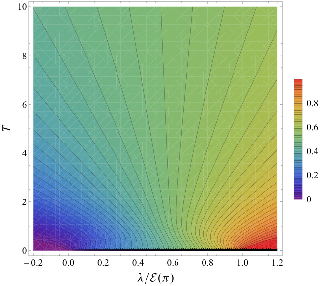
As a concrete example, we shall first focus on the elliptic chain (2)-(9). In Fig. 4 we present a contour plot of for this model with for and , obtained by numerically evaluating the integral in Eq. (34). For outside the critical interval , it is clear that is a monotonic function of (increasing for , decreasing for ), since
On the other hand, it is apparent from Fig. 4 that there is a range of values of in the interval for which the fermion density is not a monotonic function of the temperature. Remarkably, the elliptic chain exhibits this interesting behavior for all values of the parameter , including the limiting cases and . More precisely, for each there are three critical values () of the chemical potential such that: i) for , the fermion density reaches an absolute minimum at some positive temperature and then increases monotonically towards its limiting value ; ii) for , first reaches a maximum at some and then a minimum, after which it tends monotonically to ; iii) for , is monotonically increasing, and iv) for , the fermion density attains an absolute maximum at some and then decreases monotonically towards . This is also true for the limiting values (XX model) and ( HS chain), for which and , , respectively. This behavior is qualitatively apparent from Fig. 5, where we have represented the implicit curve vs. and for , and is also confirmed by the plots of vs. for these values of and presented in Fig. 6.
Although in general the integral in Eq. (34) cannot be computed in closed form, its low temperature behavior can be readily determined, as we shall now explain. To begin with, when the exponent is positive throughout the whole integration range, so that
where . Using Eq. (20) and extending the integration range to we obtain
Proceeding in a similar way we obtain an analogous formula when :
We thus see that for the fermion density at low temperature is monotonic, approaching exponentially its zero temperature values (for ) and (for ). For , the change of variable and Eq. (20) easily yield
and therefore
Likewise, at the other endpoint we have
since now is even and hence greater than .
Suppose next that lies in the critical interval . We start by writing the fermion density as the sum
where the first term is the value of at (cf. Eq. (31)). In this case the leading () contributions to the two integrals cancel each other, so that we need to evaluate the corrections. For the first integral, after performing the change of variable we have
Expanding to first order in we obtain
where we have used the expansion . We thus have
Substituting in the definition of and using the estimate
(with ) we obtain
| (35) |
The term can be similarly dealt with through the analogous change of variable , so that and hence
From the definition of we immediately obtain
and combining this result with Eq. (35) we finally have
| (36) |
In particular, for the XX and HS chains the low temperature expansion (36) reads
The absence of a term linear in in Eq. (36) is in agreement with the low temperature behavior of apparent from Fig. 6. It is also interesting to observe that the sign of the leading correction to the value of is opposite to that of the second derivative of at the Fermi momentum . This behavior can be understood by noting that the energy difference between adding a fermion with momentum (or ) and removing a fermion with momentum (or ), with , is given by . Thus when the addition of a fermion is energetically more favorable than its removal for momenta close to the Fermi momentum (or to ), and consequently the fermion density should increase at sufficiently low temperatures. For instance, for the elliptic interaction (9) with finite is positive for less than a critical momentum (which depends on ) and negative for larger momenta, while for the HS chain (i.e., for ) is always negative. Again, these facts are consistent with the behavior of observed in Fig. 6.
VII Summary and outlook
In this paper we introduce a general class of supersymmetric spin chains with long-range interactions generalizing the Haldane–Shastry and Inozemtsev (elliptic) chains, which can be fermionized using the algebraic properties of the permutation operator. We exploit this fact to study the critical behavior of this class of models (with nonzero chemical potential ) in terms of their dispersion relation . More precisely, we show that they are gapless when the chemical potential lies on the interval , and that their ground state is a product state unless belongs to this interval. We prove that the models under study are actually critical when by verifying that their low energy excitations are linear in the excitation momentum, and that their free energy at low temperature exhibits the characteristic quadratic behavior found in a -dimensional CFT with [18, 19]. As further confirmation of this critical behavior, we find an exact asymptotic formula for the von Neumann and Rényi entanglement entropies for the ground state, showing that when belongs to the open interval they both scale as when the size of the block of spins considered tends to infinity. Moreover, in both cases the constant multiplying is the same as for a -dimensional CFT with central charge [20, 21, 22]. Likewise, we show that the asymptotic behaviors of the entanglement entropy and the zero-temperature fermion density as approaches the endpoints of the critical interval are consistent with a quantum (continuous) phase transition. We also analyze the fermion density at finite temperature for a particular class of models with elliptic interactions, finding that its behavior is nontrivial (for instance, it is not always a monotonic function of the temperature, and it can in fact present up to two extrema at finite temperature) when belongs to the critical interval.
The results of this paper suggest several lines for future research. For one thing, they might prove relevant for the analogs of the models discussed in this paper, and most notably the spin Inozemtsev and HS chains in the presence of a magnetic field. Indeed, it has been analytically shown that the HS chain with zero chemical potential is equivalent in the thermodynamic limit to its counterpart with zero magnetic field [17]. More recently, a numerical computation of the free energy of the spin elliptic chain with no magnetic field suggests that this model and its version with studied in this paper are also equivalent in the thermodynamic limit [38]. If this equivalence could be extended to the case of non-zero chemical potential (or magnetic field strength, for the models), the results of this work could be used, for instance, to evaluate the ground state entanglement entropy of the spin elliptic chain and its asymptotic limit when tends to infinity.
Another line of research suggested by the present work is the study of the entanglement entropy of the low-lying states of the supersymmetric model (2) when the chemical potential lies in the critical interval . Indeed, it has been recently shown [39, 40] that in a -dimensional CFT the quotient between the entanglement entropy of an excited state created by acting on the vacuum with a primary field and that of the ground state is a universal quantity, essentially determined by the conformal weights of the field. Thus the computation of the entanglement entropy of the lowest excited states of the model (2) when , which can be constructed from the equivalent fermionic model (5), could shed some light on its underlying CFT.
Acknowledgments
This work was partially supported by Spain’s MINECO under grant no. FIS2015-63966, and by the Universidad Complutense de Madrid and Banco Santander under grant no. GR3/14-910556. PT has been partly supported by the ICMAT Severo Ochoa project SEV-2015-0554 (MINECO). JAC would also like to thank the Madrid township and the “Residencia de Estudiantes” for their financial support.
References
- [1] D. Porras and J. I. Cirac, Phys. Rev. Lett. 92, 207901 (2004).
- [2] K. Kim, M.-S. Chang, R. Islam, S. Korenblit, L.-M. Duan, and C. Monroe, Phys. Rev. Lett. 103, 120502 (2009).
- [3] P. Jurcevic, B. P. Lanyon, P. Hauke, C. Hempel, P. Zoller, R. Blatt, and C. F. Roos, Nature 511, 202 (2014).
- [4] P. Richerme, Z.-X. Gong, A. Lee, C. Senko, J. Smith, M. Foss-Feig, S. Michalakis, A. V. Gorshkov, and C. Monroe, Nature 511, 198 (2014).
- [5] P. Schauß, J. Zeiher, T. Fukuhara, S. Hild, M. Chenau, T. Macrì, T. Pohl, I. Bloch, and C. Gross, Science 347, 1455 (2015).
- [6] F. D. M. Haldane, Phys. Rev. Lett. 60, 635 (1988).
- [7] B. S. Shastry, Phys. Rev. Lett. 60, 639 (1988).
- [8] V. I. Inozemtsev, J. Stat. Phys. 59, 1143 (1990).
- [9] F. D. M. Haldane, Z. N. C. Ha, J. C. Talstra, D. Bernard, and V. Pasquier, Phys. Rev. Lett. 69, 2021 (1992).
- [10] F. D. M. Haldane, in Correlation Effects in Low-dimensional Electron Systems, Springer Series in Solid-state Sciences, Vol. 118, edited by A. Okiji and N. Kawakami (1994) pp. 3–20.
- [11] B. Basu-Mallick and N. Bondyopadhaya, Nucl. Phys. B 757, 280 (2006).
- [12] B. Basu-Mallick, N. Bondyopadhaya, and D. Sen, Nucl. Phys. B 795, 596 (2008).
- [13] B. Sutherland, Phys. Rev. B 12, 3795 (1975).
- [14] P. Schlottmann, Phys. Rev. B 36, 5177 (1987).
- [15] P. Bares and G. Blatter, Phys. Rev. Lett. 64, 2567 (1990).
- [16] Y. Kuramoto and H. Yokoyama, Phys. Rev. Lett. 67, 1338 (1991).
- [17] F. Finkel and A. González-López, J. Stat. Mech.-Theory E. 2014, P12014(28) (2014).
- [18] H. W. J. Blöte, J. L. Cardy, and M. P. Nightingale, Phys. Rev. Lett. 56, 742 (1986).
- [19] I. Affleck, Phys. Rev. Lett. 56, 746 (1986).
- [20] C. Holzhey, F. Larsen, and F. Wilczek, Nucl. Phys. B 424, 443 (1994).
- [21] P. Calabrese and J. Cardy, J. Stat. Mech.-Theory E. 2004, P06002(27) (2004).
- [22] P. Calabrese and J. Cardy, J. Stat. Mech.-Theory E. 2005, P04010(24) (2005).
- [23] Here and it what follows, all sums range from to unless otherwise stated.
- [24] E. T. Whittaker and G. N. Watson, A Course of Modern Analysis (Cambridge University Press, 1927).
- [25] F. W. J. Olver, D. W. Lozier, R. F. Boisvert, and C. W. Clark, eds., NIST Handbook of Mathematical Functions (Cambridge Univeristy Press, 2010).
- [26] S. Sachdev, Quantum Phase Transitions, 2nd ed. (Cambridge University Press, 2011).
- [27] It can be easily checked with the help of Legendre’s identity that is not an elliptic function.
- [28] F. Göhmann and M. Wadati, J. Phys. Soc. Jpn. 64, 3585 (1995).
- [29] Indeed, for , so that the error incurred in extending the upper integration limit to is bounded by for all , where is a positive constant.
- [30] G. Vidal, J. I. Latorre, E. Rico, and A. Kitaev, Phys. Rev. Lett. 90, 227902(4) (2003).
- [31] Although, strictly speaking, Eq. (25) only holds for , it is obvious that coincides with the limit of the latter equation.
- [32] M. A. Nielsen and I. L. Chuang, Quantum Computation and Quantum Information, 10th Anniversary ed. (Cambridge University Press, Cambridge, 2010).
- [33] B.-Q. Jin and V. E. Korepin, J. Stat. Phys. 116, 79 (2004).
- [34] More precisely, since we have not actually computed the entanglement entropy for exactly equal to the previous calculation only shows that the entropy has the same limit as and .
- [35] Cf. the previous footnote.
- [36] M. E. Fisher and R. E. Hartwig, Adv. Chem. Phys. 15, 333 (1968).
- [37] E. L. Basor, Indiana Math. J. 28, 975 (1979).
- [38] R. Klabbers, “Thermodynamics of Inozemtsev’s elliptic spin chain,” (2016), arXiv:1602.05133v1 [math-ph].
- [39] F. Castilho Alcaraz, M. Ibañez Berganza, and G. Sierra, Phys. Rev. Lett. 106, 201601(4) (2011).
- [40] M. Ibañez Berganza, F. Castilho Alcaraz, and G. Sierra, J. Stat. Mech.-Theory E. 2012, P01016(29) (2012).