Math. Model. Nat.
Phenom.
Vol. 3, No. 1, 2008, pp. 1-3
A Semi-Markov Algorithm
for Continuous Time Random Walk Limit Distributions
G. Gilla, P. Strakaa 11 1 Corresponding author. E-mail: p.straka@unsw.edu.au
a School of Mathematics & Statistics, UNSW Australia
Abstract. The Semi-Markov property of Continuous Time Random Walks (CTRWs) and their limit processes is utilized, and the probability distributions of the bivariate Markov process are calculated: is a CTRW limit and a process tracking the age, i.e. the time since the last jump. For a given CTRW limit process , a sequence of discrete CTRWs in discrete time is given which converges to (weakly in the Skorokhod topology). Master equations for the discrete CTRWs are implemented numerically, thus approximating the distribution of . A consequence of the derived algorithm is that any distribution of initial age can be assumed as an initial condition for the CTRW limit dynamics. Four examples with different temporal scaling are discussed: subdiffusion, tempered subdiffusion, the fractal mobile/immobile model and the tempered fractal mobile/immobile model.
Key words: anomalous diffusion, fractional kinetics, Semi-Markov, fractional derivative
AMS subject classification: 60F17, 60G22, 90C40
1. Introduction
Subdiffusion is now a well-studied theoretical phenomenon in statistical physics, motivated by experimental findings in many different fields, most prominently biophysics [1, 2, 3, 4, 5, 6]. The Continuous Time Random Walk (CTRW) has been a particularly successful model for subdiffusion [1, 7], due to both its tractability and flexibility: i) Probability densities can be computed via the fractional Fokker-Planck equation [8, 9]; ii) Reaction-subdiffusion equations can be derived from CTRW dynamics [10, 11] iii) Nonlinear dynamics may be incorporated into CTRWs [12, 13]; iv) CTRWs, via subordination, can model a variety of scaling behaviours and cross-overs between scales (see [14, 15] and Section 6 in this article); and v) Via a coupling between jumps and waiting times, an even greater variety of CTRW processes can be modeled [16, 17], with applications to Lévy Walks [18] and relaxation phenomena [19].
CTRWs and their scaling limits, however, do not possess the Markov property, but are in fact Semi-Markov processes [20]. This means that the calculation of the joint distribution at multiple times (termed “finite-dimensional distributions” in stochastic process theory) is problematic, though significant progress has been made [21, 22, 23].
In this article, we utilise the Semi-Markov property of scaling limits of CTRWs, and thus derive a computational algorithm for the calculation of the probability distributions of CTRW limit processes. Our approach uses the purely Markovian dynamics of , where is a CTRW limit process and the process which tracks the time which has passed since the last jump. This process has saw teeth sample paths (Figure 1, also see [22]) and is well-known from renewal theory as the “age” or “backward recurrence time.” Here, we shall refer to as the “residence time.”
The main conceptual difficulty with the Semi-Markov property of CTRW limits is that conditional on we almost surely have for infinitely many in for any . A careful analysis of the limiting sample paths is necessary to properly define and to establish the Markov property [20]. It is seemingly necessary to utilize jump processes with infinite Lévy measures to define the joint process . The procedure that we use to approximate these is similar to the approximation of Lévy processes by compound Poisson processes (see e.g. Section 3.4 in [24]). We walk the reader through the main technical steps in Sections 2-4.
Our algorithm (Section 5) computes the probability densities of , and by the Markov property and the Chapman-Kolmogorov equations, joint distribution of this process at multiple times can be calculated. By taking marginal distributions, one thus arrives at the joint distribution of at multiple times.
Another important application of our algorithm in the fact that any age distribution may be taken as an initial condition. This is an important generalization to the Fractional-Fokker-Planck equation, which implicitly assumes that the initial age of every particle equals . For instance, taking a snapshot of a cell in which protein molecules are undergoing (tempered) subdiffusion, there is no reason to believe that the time of the snapshot marks the beginning of a waiting time for each protein molecule. We deem it more likely that an “equilibrium” initial condition for the molecule residence times is more appropriate (Section 6).
2. CTRWs as random walks in space-time
In this section we set up the theory for scaling limits of CTRWs. Space and time need to be jointly rescaled in order to arrive at a meaningful limit, in much the same fashion as Brownian motion is the scaling limit of random walks. Which scaling functions are appropriate will depend on the tail behaviour of the waiting time and jump distributions. For simplicity, we will later assume nearest neighbour jumps, and focus on what scaling limits are appropriate for the waiting times, but the derivation in this Section is held as general as possible, which is of independent interest, and causes no extra difficulty.
The key property of CTRWs, which makes much of their analysis a great deal easier compared to e.g. fractional Brownian motion, is the renewal property: Every time a walker jumps, its entire future trajectory becomes independent of its past. The next jump time and the next position thus only depend on the current time and position; in other words, position and jump time constitute a Markov chain in space-time . The probability distribution of this Markov chain is then uniquely determined by i) its starting point in space-time and ii) a jump kernel expressing the probability that conditional on a CTRW arriving at at time , its next jump happens at time and is of size . It satisfies that
- 1.
is a probability measure on for every
- 2.
is measurable for any (Borel) .
For example, to define a subdiffusive random walk with subdiffusive coefficient in a space- and time-dependent external force field , define the transition probability kernel via
where stands for “minimum” and denotes a Gaußian probability distribution on with mean and variance . Note that the jump, occurring at time , is biased by the external force , which is accordingly evaluated at the time .
The above Markov chain defines a sequence of random points in space-time , , , from which the CTRW trajectory can be uniquely reconstructed: If , then . To avoid confusion, we stress that there are two different notions of “time”: CTRW jumps occur in physical time (which we denote by ), at epochs given by . The jumps of the space-time Markov chain occur at the integer times , which corresponds to the count of CTRW jumps. In the scaling limit below, this count becomes continuous, and we dub it the auxiliary time (usually writing ).
We identify a CTRW with its underlying space-time Markov chain. We then give conditions for a sequence of such Markov chains to converge to a continuum “jump-diffusion” process, whose state space is (Theorem 1). This convergence holds on the stochastic process level, in the sense of weak convergence of probability measures on the Skorokhod space of trajectories. Trajectories of this jump-diffusion then again map to trajectories of CTRW limit processes (Theorem 5).
Theorem 1.
For every , let be a Markov chain on the state space with starting point and a transition kernel as described above. Assume that
- 1.
(2.1) (2.2) (2.3) (2.4) where , and are real-valued bounded continuous functions, , is a Lévy measure on (see remark below) for every and is varying over all real-valued bounded continuous functions which vanish in a neighborhood of the origin .
- 2.
The operator given by
(2.5) generates a Feller semigroup of transition probabilities22 2 denotes the probability that and given , . It thus operates on continuous functions vanishing at , via . The semigroup property reads , and is equivalent to the Chapman-Kolmogorov equations for Markov processes. The Feller property is a technical condition, see e.g. [25]. on (the space of real-valued continuous functions which vanish at ).
- 3.
is an independent Poisson process with unit intensity.
Then the sequence of processes converges weakly (with respect to the Skorokhod topology) to the -valued diffusion process with jumps starting at and governed by the Feller semigroup .
A proof is given in the appendix.
Remark 2.
Remark 3.
That is a Lévy measure for every means that it is supported on and satisfies
Since all measures are supported on (i.e. waiting times are strictly positive) it follows that is in fact supported on . Readers familiar with Lévy processes will recognize that the requirement that the limiting process be strictly increasing a.s. in fact is equivalent to
Example 4.
Define the kernels via
where is the Gamma-function, , is vector valued and the unit matrix. As discussed further above, each kernel governs a CTRW process, which is subdiffusive with coefficient , meaning that waiting times have the power-law distribution
Jumps are biased according to the external force , which is evaluated at the time of a jump. It can be checked that the four limit statements from Theorem 1 are satisfied with as given, (Kronecker-delta), and (Here denotes the Dirac measure concentrated at ).
The continuum process is then such that is a -stable subordinator, i.e. a Lévy process with non-decreasing sample paths [26]. Since puts infinite measure on the positive real line, is strictly increasing, and is a diffusion process with constant diffusivity and drift given by . Its representation as a stochastic differential equation is
where is -dimensional standard Brownian motion.
3. The Semi-Markov property
We have seen that from the sequence the trajectory of a CTRW can be uniquely reconstructed. The -valued CTRW is not a Markov process, but the -valued process is; Here, is the “residence time” of a CTRW (i.e. the time which has passed since its last jump), defined as
To see the Markov property, note that for any ,
where the first equality follows from the renewal property of the CTRW, and the last equality from and on .
The following theorem shows that if the convergence
of the space-time valued processes holds as in Theorem 1, then the CTRWs & residence time processes also converge.
Theorem 5.
Let be a sequence of transition kernels on , a starting point, the corresponding sequence of CTRWs, and the sequence of residence time processes. If assumptions 1. and 2. of Theorem 1 hold and if the process has a.s. strictly increasing sample paths, then the process sequence converges weakly (with respect to the Skorokhod topology). The limiting valued process has sample paths which are right-continuous with existing left-hand limits, and is given by
where is as in Theorem 1 and
A proof is given in the appendix.
Remark 6.
The limiting process from Theorem 5 has the intuitive shorthand representation
where is the composition of trajectories and a minus / plus sign in the subscript denotes the left-continuous / right-continuous version of a trajectory.
The special case where is a strictly increasing Lévy process (i.i.d. increments) the process has continuous sample paths and is called the inverse subordinator (see e.g. [27]). In the often discussed model of subdiffusion with space- and time-dependent forcing [16], is a diffusion process, with drift evaluated at the times [28]. The time-change of by is called subordination. Theorem 5 above, however, holds in the general situation, where jumps of a walker may be coupled with (i.e. are not independent of) the waiting times in the limit as . In Example 4, there is a dependence of the jumps on the preceding waiting time , through . If the external force is evaluated at the beginning of a waiting time, another type of dependence arises, which results in different sample paths [29]; In the limit , however, this dependence vanishes. Jumps and waiting times remain coupled in the limit if and only if , where (but this is not the case in Example 4). The case where for such for all is called the uncoupled case.
Remark 7.
Example 8.
The sequence of subdiffusive CTRWs from Example 4 thus converges to the process , and according to Remark 7 . The probability densities of , if they exist, solve the fractional Fokker-Planck equation
where the Fokker-Planck operator is given by
(compare [8, 30, 31]). Note that since is the start of a waiting time for all particles, the initial condition assumes that all particles have age , i.e. that .
4. Discrete Semi-Markov Processes
Theorems 1 and 5 provide limit theorems which are applicable to a large class of CTRW limits, and show that the Markov property holds for CTRWs as well as for their limit processes. In this section, we assume that a CTRW limit process is given, and construct a sequence of discrete CTRWs which converges to . Any member assumes values on a discrete spatial lattice, in a fashion similar to [29]. Rather than integrating into the history of , however, our goal here is to implement the Markovian dynamics of , and thus to become able to directly incorporate distributions of residence times into the initial condition. With discrete Markovian dynamics, the master equations for the evolution of probability functions of can then be straightforwardly implemented, see the next section.
Simplifying Assumptions.
Recall that according to Theorem 1, a CTRW limit process is characterized by the coefficient functions , , and the space-time Lévy kernel . For simplicity, we narrow down the class of CTRW limits that we consider in the remainder of this article. We assume only nearest neighbor jumps on the spatial lattice, which entails that the Lévy measures have the representation for some measures on , and the dynamics are uncoupled. We further assume that , i.e. waiting times are homogeneous. To avoid speaking of degenerate CTRW limits, we assume that the measure is infinite (i.e. has a non-integrable singularity at , even though )33 3 Indeed, if is a finite measure, then the process is a step process, and hence the limiting CTRW is again a CTRW.. Finally, we focus on the one-dimensional case and assume that and are constant.
Instead of working with the measure , it is more convenient in our setting to analyse the (right-continuous) tail function instead. Then infiniteness of translates to , and the Lévy measure property to , as can be seen by integration by parts. The typical example to have in mind is for , and (subdiffusion). To arrive at a computational algorithm for the master equations for the laws of , we need to give a sequence of transition kernels which are supported on a lattice, and which satisfy (2.1)–(2.4). With this in mind, we define
| (4.1) |
where we define the ceiling function as . The constants and depend on and are defined as follows:
It can then be checked that , that is right-continuous and decreases to as . Thus is the tail function of a probability measure supported on the lattice . Since is of finite variation, one can define the Lebesgue-Stieltjes measure via . Note however, that since is decreasing, this measure is negative. Since is piecewise constant, with jumps in the set , is a discrete probability measure on . Finally, define a sequence of CTRW processes (and their residence time processes ) via their transition kernel:
| (4.2) |
The probabilities and to jump right/left need of course to be positive, which is satisfied for small enough . Given a starting point on the lattice , the CTRW will remain on this lattice at all times. Moreover, if the starting time is chosen from the lattice , then all jump times will also lie on this lattice.
Lemma 9.
Let and be as above. Then the following two equalities hold:
where ranges over all real-valued differentiable functions with compact support in .
A proof is given in the appendix. The following result may be interpreted as the consistency of our discrete Semi-Markov scheme:
Theorem 10.
Let the simplifying assumptions as set out above hold, and consider the sequence of discrete CTRWs with residence time processes , for , defined via the kernels (4.2) and starting point at time . Then converges44 4 You guessed it! Weakly with respect to Skorokhod’s topology. to the process as given in Theorem 5. That is, , where
- i)
is a diffusion process with constant diffusivity and drift , with
- ii)
is an independent subordinator (strictly increasing Lévy process) with drift and Lévy measure , and
- iii)
is the inverse subordinator.
The process tracks the residence time of , and satisfy the Markov property.
Proof.
For large , we may hence assume that the distribution of for will be a good approximation for the distribution of the of the CTRW limit . In the next section we compute these distributions.
5. Algorithm
We can now derive a time-stepping algorithm which calculates the probability functions of the discrete process , whose state space is , and whose time-steps lie in . Recall that for , denotes the probability that a waiting time of the CTRW is or longer. Therefore conditioning on , we are conditioning on the waiting time being longer than , that is or longer. Hence observing the transition kernel (4.2) we find:
| (5.1) | ||||
where , and where we set . Writing
we may then write a master equation for the evolution of these probabilities: The first term on the right-hand side of (5.1) corresponds to the case where a particle remains on its site for another time step , and hence we have
The second term corresponds to the complementary case: a particle jumps to one of the neighboring lattice sites or , and its age is reset to . At a given lattice site the probability mass is hence obtained by a weighted sum over all residence times of the neighbouring lattice sites:
The CTRW limit density of the process can then be approximated through
In practice, the algorithm runs on a finite grid
representing the state space, and one has to impose additional boundary conditions.
Spatial Boundary conditions.
We only consider the one-dimensional case. For absorbing, or Dirichlet boundary conditions where is a boundary point, a walker is removed if it walks off the lattice. That is, we set and for all , ; note that on the boundary site, and hence no longer add to .
For reflecting, or Neumann boundary conditions, a particle remains at a boundary site whenever it would jump off the lattice, and adjust (4.2) accordingly.
Residence time boundary conditions.
When the residence time of a particle approaches the lattice end at , we could force it to jump to a neighboring lattice site and reset its age to . This effectively corresponds to a tail function , and hence we term this the cutoff boundary condition.
Below, however, we assume that upon reaching the end of the lattice at , a particle is not forced to jump, and allow it to remain at its site with residence time if it would not otherwise jump. That is, we set
This means that particles with residence time remain unchanged for a geometrically distributed number of time steps, with parameter . In the scaling limit, this corresponds to an exponential distribution, whose rate is
(note that as , we have and ). This effectively corresponds to a tail function
and hence we term this procedure the cross-over boundary condition.
Assume now as a general initial condition a probability measure , and that the aim is to calculate
To this end, we set , and simply run our algorithm with this initial condition. Note that needs to be chosen large enough in order to avoid cut-off or cross-over effects for as discussed above. A safe choice is always
where denotes the number of time steps, though it may of course be infeasible in cases where has unbounded support.
6. Examples
Within our framework, we may now compute (approximations of) probability distributions of CTRW limits, with varying initial residence times, for a variety of models. In particular, we may assume any subordinator , and thus treat a variety of non-Markovian behaviours (see Table 1). Two main regimes occur, depending on whether has integrable tails or not. In the former case, admits the equilibrium distribution
| (6.1) |
where and denotes a Dirac measure at [32]. In the latter case, there exists an invariant measure, but it is infinite, and hence an equilibrium cannot be reached.
Tempering.
Throughout, . The tail function in the subdiffusive case is not integrable. The tempered subdiffusive case is obtained by multiplying the Lévy density with an exponential [33]. The tail function becomes
where denotes the upper incomplete Gamma function. This modification makes integrable for , that is, . CTRW limits with these “tempered dynamics” appear subdiffusive on short time scales and diffusive on longer time scales [14, 34, 35]. Note that for the above reduces to the subdiffusive case.
Subordinator with drift.
If the subordinator has a positive drift constant , the resulting growth of at very short times is proportional to . Accordingly, the inverse subordinator also grows linearly, proportionally to for short times55 5 A law of the iterated logarithm applies for the precise limit, see [26].. For larger time scales, the jumps of will dominate the drift , if (or if in the case where is not integrable). This means that for long times, the temporal evolution appears subdiffusive if [34]. The case and has been examined in [34]: grows linearly for small time scales. For long time scales, also grows linearly, although with a smaller slope. To our knowledge, the cross-over between the two regimes at intermediate time scales has not been looked at in detail but we predict it will show the signatures of subdiffusive behavior.
Finally, in the case where and , by the above , and and admit a nice physical interpretation: At equilibrium, is the fraction of “mobile” particles which have residence time , and is the fraction of “immobile” particles, which have been trapped for a time distributed as . We deem this to be an interesting tempered extension of the so called “fractal mobile/immobile model” of [15]. If , there exists no equilibrium, and all mobile particles eventually seep into the immobile phase.
| model | tempering parameter | temporal drift |
|---|---|---|
| Subdiffusion | ||
| tempered subdiffusion | ||
| fractal mobile-immobile | ||
| tempered fractal mobile-immobile |
Varying the initial residence time.
When modelling subdiffusion or tempered subdiffusion, the standard assumption is that the first waiting time starts at , which translates to the initial condition (all particles have residence time , and their location is distributed according to , typically , [8]). Subdiffusive CTRWs are known to exhibit ageing, which is an indefinite slowing down of the dynamics as increases. [36] consider dynamics of CTRW limits where the system has been prepared at a time , and study the dynamics on the interval , for which e.g. a Fokker-Planck equation has been derived in [37]. This relates to our approach by taking as initial condition the probability distribution , and calculating the probability distributions of for .
In the subdiffusive setting, we now examine the impact of a varying initial residence time on the probability function of a CTRW limit. In particular, we calculate the “Green’s functions” where . For simplicity, we assume symmetric nearest neighbor jumps with reflecting boundary condition, and a fractional parameter . Figure 2, with shows the distinctive cusp shape of the probability density of subdiffusive CTRW limits (see e.g. [1]). On the other hand, if conditioning on and where is positive, the particle is trapped at , and stays there until time with probability ; Compare [20, Th 4.1] which provides a formula for the conditional distribution . Hence the joint distribution of , conditioned on , has an atom of mass at . This atom reflects in the marginal distribution of , as shown in Figures 2 and 3. The remaining probability mass, as given in [20, Th 4.1], is absolutely continuous. As , the weight of this atom increases towards .
Evolution of the residence time distribution.
Figure 3 describes the evolution of the densities of the residence time process . Again we consider the subdiffusive case with as in the previous paragraph. If , we have due to self-similarity , and the distribution of follows the arcsine law
compare [26, Prop 3.1]. If , the distribution of has an atom at , whose weight increases to as , compare the discussion in the previous paragraph. In the tempered case, for the distribution approaches (6.1).
Computational accuracy.
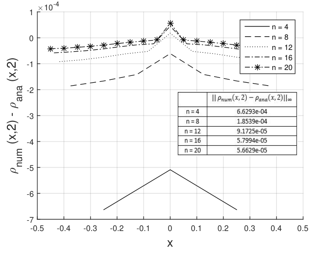
Exact analytical solutions to the symmetric subdiffusion equation are available, and we check our computed densities against these solutions. Following [29], use the series representation
for the solution to the “standard” fractional diffusion equation
As shown e.g. in [8], the corresponding CTRW limit process is given by symmetric nearest neighbor jumps, and . Figure 4 displays the computational errors for this case, which seem to stabilize as the densities of the discrete CTRW approach the CTRW limit (as ).
7. Conclusion
Similar in spirit to [29], we have derived an algorithm for the computation of probability distributions of CTRW limits, which is based on the stochastic process rather than the fractional Fokker-Planck equation. Additionally, our approach calculates the residence time, or age of a walker, which is of independent physical interest, and which may be of use for the modelling of non-Markovian diffusion with distributed age initial condition.
In [38] it is shown that the discrete stochastic processes approach from [29] is also applicable to model reaction-diffusion problems and nonlinear interactions. Our approach above assumes that particles do not interact, and there are severe technical obstacles in extending the above mathematical rigour to CTRW limit processes which interact via reactions, chemotaxis, or otherwise. It is straightforward, however, to write down master equations with interactions using the Semi-Markov formalism, and thus to calculate mass distributions, see [12]. The work here may be viewed as an extension to [12] which can model general subordinated particle dynamics.
In order to focus on the main ideas, we have only considered CTRWs with nearest neighbor jumps and homogeneous waiting times. By varying the coefficients , , and and by possibly making them vary in space and time, one can arrive at a variety of different models; for three such models, see [30]. It is possible to generalize the Semi-Markov algorithm from Section 5 to coupled and non-local jump operators, given the formulas derived in [20], though this may of course require much larger computational effort.
Acknowledgements
P. Straka was supported by the UNSW Science Early Career Research Grant and the Australian Research Council’s Discovery Early Career Research Award.
References
- [1] Ralf Metzler and Joseph Klafter. The random walk’s guide to anomalous diffusion: a fractional dynamics approach. Phys. Rep., 339(1):1–77, dec 2000.
- [2] Benjamin M. Regner, Dejan Vučinić, Cristina Domnisoru, Thomas M. Bartol, Martin W. Hetzer, Daniel M. Tartakovsky, and Terrence J. Sejnowski. Anomalous Diffusion of Single Particles in Cytoplasm. Biophys. J., 104(8):1652–1660, apr 2013.
- [3] Brian Berkowitz, Andrea Cortis, Marco Dentz, and Harvey Scher. Modeling non-Fickian transport in geological formations as a continuous time random walk. Rev. Geophys., 44(2):RG2003, 2006.
- [4] Enrico Scalas. Five Years of Continuous-time Random Walks in Econophysics. Complex Netw. Econ. Interact., 567:3–16, jan 2005.
- [5] Fidel Santamaria, Stefan Wils, Erik De Schutter, and George J. Augustine. Anomalous diffusion in Purkinje cell dendrites caused by spines. Neuron, 52(4):635–48, nov 2006.
- [6] Daniel S. Banks and Cécile Fradin. Anomalous diffusion of proteins due to molecular crowding. Biophys. J., 89(5):2960–71, nov 2005.
- [7] Bruce I Henry, Trevor AM Langlands, and Peter Straka. An introduction to fractional diffusion. In R L. Dewar and F Detering, editors, Complex Phys. Biophys. Econophysical Syst. World Sci. Lect. Notes Complex Syst., volume 9 of World Scientific Lecture Notes in Complex Systems, pages 37–90, Singapore, 2010. World Scientific.
- [8] B I Henry, T. A. M. Langlands, and Peter Straka. Fractional Fokker-Planck Equations for Subdiffusion with Space- and Time-Dependent Forces. Phys. Rev. Lett., 105(17):170602, 2010.
- [9] T.A.M. Langlands and B.I. Henry. The accuracy and stability of an implicit solution method for the fractional diffusion equation. J. Comput. Phys., 205(2):719–736, may 2005.
- [10] Vicenc Mendez, Sergei Fedotov, and Werner Horsthemke. Reaction-Transport Systems: Mesoscopic Foundations, Fronts, and Spatial Instabilities. Springer Berlin/Heidelberg, 1st edition, jun 2010.
- [11] Christopher N Angstmann, I C Donnelly, and B.I. Henry. Continuous Time Random Walks with Reactions Forcing and Trapping. Math. Model. Nat. Phenom., 8(2):17–27, apr 2013.
- [12] Peter Straka and Sergei Fedotov. Transport equations for subdiffusion with nonlinear particle interaction. J. Theor. Biol., 366:71–83, feb 2015.
- [13] Sergei Fedotov and Nickolay Korabel. Self-organized anomalous aggregation of particles performing nonlinear and non-Markovian random walks. Phys. Rev. E, 92(6):062127, dec 2015.
- [14] Aleksander Stanislavsky, Karina Weron, and Aleksander Weron. Diffusion and relaxation controlled by tempered -stable processes. Phys. Rev. E, 78(5):6–11, nov 2008.
- [15] Rina Schumer, David A Benson, Mark M. Meerschaert, and Boris Baeumer. Fractal mobile/immobile solute transport. Water Resour. Res., 39(10), oct 2003.
- [16] Peter Straka and B I Henry. Lagging and leading coupled continuous time random walks, renewal times and their joint limits. Stoch. Process. their Appl., 121(2):324–336, feb 2011.
- [17] A. Jurlewicz, P. Kern, Mark M. Meerschaert, and H.P. P. Scheffler. Fractional governing equations for coupled random walks. Comput. Math. with Appl., 64(10):3021–3036, nov 2012.
- [18] Marcin Magdziarz, H.P. Scheffler, Peter Straka, and P. Zebrowski. Limit theorems and governing equations for Lévy walks. Stoch. Process. their Appl., 125(11):4021–4038, 2015.
- [19] K. Weron, A. Jurlewicz, Marcin Magdziarz, A. Weron, and J. Trzmiel. Overshooting and undershooting subordination scenario for fractional two-power-law relaxation responses. Phys. Rev. E, 81(4):1–7, apr 2010.
- [20] Mark M. Meerschaert and Peter Straka. Semi-Markov approach to continuous time random walk limit processes. Ann. Probab., 42(4):1699–1723, jul 2014.
- [21] Ofer Busani. Finite Dimensional Fokker-Planck Equations for Continuous Time Random Walks. arXiv 1510.01150, oct 2015.
- [22] Mark M. Meerschaert and Peter Straka. Fractional Dynamics at Multiple Times. J. Stat. Phys., 149(5):878–886, nov 2012.
- [23] A. Baule and R. Friedrich. A fractional diffusion equation for two-point probability distributions of a continuous-time random walk. Europhys. Lett., 77(1):10002, jan 2007.
- [24] Mark M. Meerschaert and Alla Sikorskii. Stochastic models for fractional calculus. De Gruyter, Berlin/Boston, 2011.
- [25] D. Applebaum. Lévy Processes and Stochastic Calculus, volume 116 of Cambridge Studies in Advanced Mathematics. Cambridge University Press, 2nd edition, may 2009.
- [26] Jean Bertoin. Subordinators: examples and applications, volume 1717 of Lecture Notes in Mathematics. Springer Berlin Heidelberg, Berlin, Heidelberg, 1999.
- [27] Mark M. Meerschaert and Peter Straka. Inverse Stable Subordinators. Math. Model. Nat. Phenom., 8(2):1–16, 2013.
- [28] A. Weron and Marcin Magdziarz. Modeling of subdiffusion in space-time-dependent force fields beyond the fractional Fokker-Planck equation. Phys. Rev. E, 77(3):1–6, mar 2008.
- [29] Christopher N Angstmann, I C Donnelly, B.I. Henry, T.A.M. Langlands, and Peter Straka. Generalized Continuous Time Random Walks, Master Equations, and Fractional Fokker–Planck Equations. SIAM J. Appl. Math., 75(4):1445–1468, jan 2015.
- [30] Boris Baeumer and Peter Straka. Fokker–Planck and Kolmogorov Backward Equations for Continuous Time Random Walk scaling limits. Proc. Amer. Math. Soc., arXiv 1501.00533, jan 2016.
- [31] Marcin Magdziarz, Janusz Gajda, and Tomasz Zorawik. Comment on Fractional Fokker-Planck Equation with Space and Time Dependent Drift and Diffusion. J. Stat. Phys., 154(5):1241–1250, 2014.
- [32] Joseph Horowitz. Semilinear Markov processes, subordinators and renewal theory. Z. Wahrsch. Verw. Geb., 24(3):167–193, 1972.
- [33] Jan Rosiński. Tempering stable processes. Stoch. Process. Appl., 117(6):677–707, jun 2007.
- [34] Peter Straka. Continuous Time Random Walk Limit Processes: Stochastic Models for Anomalous Diffusion, available at http://unsworks.unsw.edu.au/fapi/datastream/unsworks:9800/SOURCE02. PhD thesis, University of New South Wales, 2011.
- [35] Janusz Gajda and Marcin Magdziarz. Fractional Fokker-Planck equation with tempered alpha-stable waiting times: Langevin picture and computer simulation. Phys. Rev. E, 82(1):1–6, jul 2010.
- [36] Eli Barkai and Yuan-Chung Cheng. Aging continuous time random walks. J. Chem. Phys., 118(14):6167, 2003.
- [37] Ofer Busani. Aging uncoupled continuous time random walk limits. arXiv, 1402.3965, feb 2015.
- [38] Christopher N Angstmann, Isaac C Donnelly, Bruce I Henry, BA Jacobs, Trevor AM Langlands, and James A Nichols. From stochastic processes to numerical methods: A new scheme for solving reaction subdiffusion fractional partial differential equations. J. Comput. Phys., 307:508–534, 2016.
- [39] Jean Jacod and Albert N Shiryaev. Limit Theorems for Stochastic Processes. Springer, dec 2002.
- [40] P. Billingsley. Convergence of Probability Measures. Wiley Series in Probability and Statistics. John Wiley & Sons Inc, New York, second edition, jan 1968.
- [41] Edwin Hewitt. Integration by Parts for Stieltjes Integrals. Am. Math. Mon., 67(5):419, may 1960.
Appendix A Proofs
Proof of Theorem 1.
Proof of Theorem 5.
We apply Proposition 2.3 in [16], which states the following: The mapping
defined for càdlàg66 6 French acronym for right-continuous with left-hand limits trajectories and in resp. , where is increasing and unbounded, and where , is continuous at all trajectories where is strictly increasing. As before, denotes a composition of trajectories, and a in the subscript denotes the right-continuous resp. left-continuous version of a trajectory. Continuity is with respect to the (metrizable) Skorokhod topology on the set of all such trajectories [39].
Next, apply the continuous mapping theorem [40]: Since the processes converge to as , and is strictly increasing (almost surely), the sequence of their images must converge to the image . Here, , , and (note that has a.s. increasing sample paths). It is tedious but not too difficult to check that and are really the images of and for the above mapping.
Finally, in a similar fashion mapping the process to the process also defines a continuous mapping, hence also converges to . ∎
Proof of Lemma 9.
The measure is concentrated at the steps of the function . We use this and Lebesgue-Stieltjes integration by parts [41] to calculate
Now examine these terms individually as :
where means the two sequences have the same limit. By dominated convergence, the integral of the third expression converges to . Since is integrable at , at where . Hence . Now letting gives the first statement.
The second statement follows by integration by parts and dominated convergence:
(note that the boundary terms vanish by definition of ). ∎