Scalable Linear Causal Inference for Irregularly Sampled Time Series with Long Range Dependencies
Abstract
Linear causal analysis is central to a wide range of important application spanning finance, the physical sciences, and engineering. Much of the existing literature in linear causal analysis operates in the time domain. Unfortunately, the direct application of time domain linear causal analysis to many real-world time series presents three critical challenges: irregular temporal sampling, long range dependencies, and scale. Moreover, real-world data is often collected at irregular time intervals across vast arrays of decentralized sensors and with long range dependencies [1] which make naive time domain correlation estimators spurious [2]. In this paper we present a frequency domain based estimation framework which naturally handles irregularly sampled data and long range dependencies while enabled memory and communication efficient distributed processing of time series data. By operating in the frequency domain we eliminate the need to interpolate and help mitigate the effects of long range dependencies. We implement and evaluate our new work-flow in the distributed setting using Apache Spark and demonstrate on both Monte Carlo simulations and high-frequency financial trading that we can accurately recover causal structure at scale.
1 Introduction
The analysis of time series is central to applications ranging from statistical finance [3, 4] to climate studies [5] or cyberphysical systems such as the transportation network [6]. In many of these applications one is interested in estimating the mutual linear predictive properties of events from time series data corresponding to a collection of data streams each of which is a series of pairs (timestamp, observation).

In most applications, observations occur at random, unevenly spaced and unaligned time stamps. In such a setting we therefore consider two underlying processes and that are only observed at discrete and finite timestamps in the form of two collections of data points: . We adapt our definition of causality to this different theoretical framework. Let be a causal convolution kernel with delay (i.e. whenever ), and two continuous time stochastic processes, for instance, two Wiener processes. A popular instance of a causation kernel is for instance the exponential kernel: We assume for instance that is an Ornstein-Uhlenbeck process or a Brownian motion (Wiener process) [7] and
| (1) |
where and are two independent Brownian motions whose increments are classically referred to as the innovation process. In the following, the parameter will be referred to as lag. We will consider that is lagging with characteristic delay behind which is causing it.
We adopt the cross-correlogram based causality estimation approach developed in [8], in order to be consistent with Granger’s definition of causality as linear predictive ability of and for the random variable [9].
Let and be two Wiener processes. We consider that has a causal effect on if is a more accurate linear predictor of in square norm error than is an accurate linear predictor of . In other words causes if and only if
| (2) |
In order to quantify the magnitude of this statistical causation, Huth and Abergel introduced in [8] the Lead-Lag Ratio (LLR) between and as
| (3) |
where is the cross-correlation between the second order stationary processes and . The analysis conducted in [8] proved causes is equivalent to
thereby yielding an indicator of causation intensity between processes which depends through (1).
1.1 Challenges with real world data:
Unfortunately, in practical applications, time series data sets often present three main challenges that hinder the estimation of even linear causal dependencies:
- •
Irregular Sampling: Observations are collected at irregular intervals both within and across processes complicating the application of standard causal inference techniques that rely on evenly spaced timestamps that align across processes.
- •
Long Range Dependencies (LRD): Long range dependencies can result in increased and non vanishing variance in correlation estimates.
- •
Scale: Real-world time series are often very large and high dimensional and are therefore often stored in distributed fashion and require communication over limited channels to process.
In the following we show as in [8] that naive interpolation of irregularly sampled data may yields spurious causality inference measurements. We also prove that eliminating LRD is crucial in order to obtain consistent correlation estimates. Unfortunately, standard time domain LRD erasure requires sorting the data chronologically and is therefore costly in the distributed setting. These costs are further exacerbated by time domain fractional differentiation which scales quadratically with the numbers of samples.
To address these three critical challenge we propose a Fourier transform based approach to causal inference. Projecting on a Fourier basis can be done with a simple sum operator for irregularly sampled data as described in [10]. A novel and salient byproduct of our estimation technique is that there is no need to sort the data chronologically or gather the data of different sensors on the same computing node. We use Fourier transforms as a signal compressing representation where cross-correlations and causal dependencies can be estimated with sound statistical methods all while minimizing memory and communication overhead. In contrast to sub-sampling in which aliasing obscures short-range interactions, our methods does not introduce aliasing enabling the study of sort-range interactions. An exciting aspect of compressing by Fourier transforms is that it only affects the variance of the cross-correlogram without destroying the opportunity to study inter-dependencies at a small time scale.
In section 2 we show that leveraging the frequency domain representation we present communication avoiding consistent spectral estimators [11] for cross-dependencies. We first compress the time series by projecting without interpolation or reordering directly onto a reduced Fourier basis, thereby locally compressing the data. Spectral estimation then occurs in the frequency domain prior to being translated back into the time domain with an inverse Fourier transform. The resulting output can be used to compute unbiased Lead-Lag Ratios and thereby identify statistical causation.
In section 3, we provide a method to approximately erase LRD in the frequency domain, which has tremendous computational advantages as opposed to time domain based methods. Our analysis of LRD erasure as fractional pole elimination in frequency domain guarantees the causal estimates we obtain are not spurious unlike those calculated naively on LRD processes [1, 2]. Finally, we apply these methods to synthetic data and several terabytes of real financial market trade tables.
In section 4, we present a novel analysis of the trade-off between estimator variance and communication bandwidth which precisely assesses the cost of compressing time series prior to analyzing them. A three-fold analysis establishes the statistical soundness of the contributions that address the three issues mentioned above. Studying data on compressed representations comes at an expected cost. In our setting this supplementary variance can be decreased in an iterative manner and with bounded memory cost on a single machine. These properties cannot be replicated to the best of our knowledge by time domain based sub-sampling.
2 Interpolation and spurious lead-lag
In this section, we first review existing techniques for interpolated time-domain estimation of second-order statistics in the context of sparse and random sampling along the time axis. Interpolating data is a usual solution in order to be able to use classic time series analysis [10, 12, 13, 14]. Unfortunately it is not always suitable, as it can create spurious causality estimates and implies a supplementary memory burden.
2.1 Second order statistics and interpolated data
In order to infer a linear model from cross-correlogram estimates by solving the Yule-Walker equations [15] or to compute a LLR (Eq. (3)) one needs to estimate the cross-correlation structure of two time series. Let and be two centered stochastic processes whose cross-covariance structure is stationary:
| (4) |
If data is sampled regularly a consistent estimator for is:
| (5) |
(we use to denote an estimator for ). Classically, cross-correlation estimates can subsequently be computed as
| (6) |
using any consistent cross-covariance estimator.
Interpolating irregular records:
The standard consistent estimator Eq. (5) cannot be computed when and do not share common timestamps. A classical way to circumvent the irregular sampling issue is therefore to interpolate the records and onto the set of timestamps therefore yielding two approximations and that can be studied as a synchronous multivariate time series. An adapted cross-covariance estimate is then While there are many interpolation techniques, a commonly used method is last observation carried forward (LOCF). Note that interpolation may require substantial additional memory to render each time series at the resolution of interactions which can be millisecond scale in many crucial applications such as studying stock market interactions.
We now consider the causality inference framework introduced in [8] and show how the LOCF interpolation technique creates spurious causality estimates.
Bias in LLR with irregularly sampled data: The can be computed by several methods. Cross-correlation measurements on a symmetric centered interval are sufficient statistics for this estimator. Therefore one can use synchronous cross-correlation estimates on interpolated data in order to compute the . Carrying the last observation forward (LOCF) has been proven to create a bias in lag estimation in [8]. The LOCF interpolation method introduces a causality estimation bias in which a process sampled at a higher frequency will be seen as causing another process which is sampled less frequently although these correspond to Brownian motions with simultaneously correlated increments.
2.2 Interpolation-free causality assessment
The Hayashi-Yoshida (HY) estimator was introduced in [16] to address this spurious causality estimation issue. The HY estimator of cross-correlation does not require data interpolation and has been proven to be consistent with processes sampled on a quantized grid of values [17] in the context of High Frequency statistics in finance.
Correlation of Brownian motions: HY is adapted to measuring cross-correlations between irregularly sampled Brownian motions. Considering the successor operator for the series of timestamps of a given process, let and be the set of intervals delimited by consecutive observations of and respectively. The Hayashi-Yoshida covariance estimator over the covariation of and [7] is defined as
| (7) |
where is true if and only if and overlap. The estimator can be trivially normalized so as to yield a correlation estimate.
HY and fractional Brownian motions: No interpolation is required with HY but unfortunately this estimator is only designed to handle full differentiation of standard Brownian motions. Figure 2 shows how HY fails to estimate cross-correlation of increments on a fractional Brownian motion whereas the technique we present succeeds. In the following, we show how our frequency domain based analysis naturally handles irregular observations and is able to fractionally differentiate the underlying continuous time process. This is in particular necessary when one studies factional Brownian motions with correlated increments. In the interest of concision, we refer the reader to [18] for the definition of a fractional Brownian motion.
 |
 |
2.3 Fourier transforms for irregularly sampled data
Our alternative approach to estimating cross-correlograms is based on the definition of the Fourier transform of a stochastic process. Considering a continuous time stochastic process and a frequency , the Fourier projection of for the frequency is defined as
| (8) |
where is the imaginary number. Much attention has been focused on the benefits of the FFT algorithm which has been designed for the very particular base of ordered and regularly sampled observations. Our key insight is to go back to the very definition of the Fourier transform as an integral and express it empirically in summation form [11, 10]. Moreover, if the process is observed at times , one can estimate the Fourier projection by
| (9) |
Therefore we propose the following simple framework for frequency domain based linear causal inference:
- 1.
Project and on to a reduced Fourier basis.
- 2.
Estimate the cross-spectrum of and in the frequency domain.
- 3.
Apply the inverse Fourier transform to the cross-spectrum to recover the cross-correlogram and infer the linear causal structure.
The intuition behind this estimation method is a change of basis that allows us to compute cross-covariance estimates without needing to address the irregularity of timestamps. Indeed the power spectrum is the element-wise Fourier transform of
Therefore, in order to estimate this function one may infer what corresponds to its frequency domain representation and then compute the inverse Fourier transform of the result.
Projecting onto Reduced Fourier Basis: We first project and onto the elements of the Fourier basis of frequencies , namely the pair and . By projecting onto a single relatively small set of orthonormal functions, we are able to compress and effectively re-align the observations and . In practice using only a few thousand basis functions we are able to accurately recover the cross-correlogram. Finally, this computation is sufficiently fast to execute interactively on a single laptop and can be easily expressed using the map-reduce framework.
Estimating the Cross-spectra: Computing projections onto a reduce Fourier basis enables exploratory data analysis through the study of the cross-spectrum of and
| (10) |
An inconsistent estimator for the cross-spectrum is:
| (11) |
Local averaging of Eq. (11) with respect to frequencies is widely used [11, 15, 10] in cross-spectral analysis to identify the characteristic frequencies at which stochastic processes interact although they are observed at irregular times. Unfortunately, to compute characteristics delays or LLR (crucial steps in linear causal inference) we still need to estimate the cross-correlogram.
Estimating the Cross-correlogram: To estimate the cross-correlogram we can take the inverse Fourier transform of the cross-spectrum which translates frequency analysis back into the time domain:
| (12) |
Using the following consistent estimator:
| (13) |
of the cross-covariance we can directly compute a consistent estimator of the cross-correlation using equation Eq. (6). The cross-correlation between and can now be estimated in the time domain with a discrete grid of lag values ranging from to with a resolution . As expected, aliasing will occur if the user specifies a resolution in the cross-correlation estimate that is much higher than the average sampling frequency of the time series [10].
In contrast to more cumbersome time domain synchronization relying on interpolation based methods (LOCF) or interval matching based estimations (HY), our method elegantly addresses time synchronization in the frequency domain. While earlier work [10, 11] has considered the application of frequency domain analytics to irregularly sampled data, our method is the first to translate back to the time domain to recover a consistent estimator of correlation. Alternatively, Lomb-Scargle periodogram [19, 20] also enables the frequency domain analysis of irregularly observed data but suffers from the supplementary cost of a least square regression. To the best of our knowledge we are the first to use frequency domain projections to compute the cross-correlogram in order to infer linear causal structure.
2.4 The statistical cost of compression
Central to the communication and memory performance of our technique is the ability to use a small number of Fourier projections relative to the number of observations and still accurately recover the cross-correlogram.
Cross-correlogram Estimator Consistency: We can characterize the statistical properties of the cross-spectral estimator [11, 10, 15]. In particular, it is well known that for two distinct non-zero frequencies and the estimators and are asymptotically independent. Consequently, to obtain an estimator with variance the user will need to project on frequencies. We confirm this result numerically in Figure 6. The element-wise product of Fourier transforms is converted into the time domain by the inverse Fourier transform to yield a cross-correlogram. With very large datasets in which we obtain the suitable compression property of our algorithm.
Issues with Non-smooth Cross-correlograms: As expected, deterministic lags or seasonal components can result in Fourier compression artifacts in the inverse Fourier transform. However, statistical estimation and removal of these deterministic components is standard in time series analysis [15, 11]. In the context of estimating non-trivial stochastic causal relationships (e.g., social networks, pairs of stock prices the financial markets, cyberphysical systems) random perturbations affect the causation delay. In these settings, the theoretical cross-correlation function is smooth. As a consequence, a few Fourier projections suffice to accurately represent the cross-correlogram in frequency domain.
2.5 Example of time domain exploratory data analysis through the frequency domain
The time domain exploratory analysis we enable makes lead-lag relationships self-explanatory as shown in Figure 1. We show in the following that it is not hindered by biases related to the fact that one process is sampled more seldom than the other.
Numerical assessment of frequency domain based correlation measurements: We demonstrate, through simulation, that the spurious causation issue that plagues the LOCF interpolation [8] does not appear in our proposed method. We consider two synthetic correlated Brownian motions that do not feature any lead-lag and compare the estimation of LLR provided by two time domain interpolation methods and our approach. After having sampled these at random timestamps, in Table 1 and Figure 3 we compare the cross-correlation and LLR estimates obtained by LOCF interpolation and our proposed frequency domain analysis technique confirming that our method does not introduce spurious causal estimation bias.
| LOCF interpolation LLR | Fourier transform LLR | |
|---|---|---|
| Avg +- std | Avg +- std | |
| , |
| LOCF cross-correlation | Fourier cross-correlation |
|---|---|
 |
 |
 |
 |
 |
 |
3 The Long Range Dependence (LRD) Issue
A stochastic process is said to be long range dependent if it features cross-correlation magnitudes whose sum is infinite [1]. Many issues arise in that case with correlation estimates becoming spurious. This phenomenon was first discover when Granger studied the concept of cointegration between Brownian motions (integrated time series) [2]. On sorted Brownian motion data, this effect can be addressed by differentiating the time series, namely computing . For fractional Brownian motion and LRD time series, the fractional differentiation operator needs to be computed. It is defined as
| (14) |
Therefore, to study the cross-correlation structure of two integrated or fractionally integrated time series, one would have to compute or . The latter requires chronologically sorted data and synchronous timestamps and has a quadratic time complexity with respect to the number of samples.
3.1 Erasing memory in the frequency domain
Erasing memory is of prime importance, in the case of the study of Brownian motions and fractional Brownian motions alike. As pointed out in [1], LRD arises in many systems, in particular those managed by humans, because of their ability to learn from previous events and therefore keep of memory of these in their future actions. From a computational and statistical point of view, it is challenging to erase.
Equivalence between differentiation in time domain and element-wise multiplication in frequency domain: Let be a continuous process whose fractional differentiate of degree , is Lebesgue-integrable with probability . If vanishes at the boundaries of the interval, classically, almost surely,
by a stochastic integration by part. Therefore, an estimate for is
Erasing memory through fractional pole elimination: The power spectrum of a fractional Brownian motion [18] with Hurst exponent is asymptotically for . This is the characteristic spectral signature of a long range dependent time series. can therefore be estimated by the classical periodogram method for an individual time series by conducting a linear regression on the magnitude of the power spectrum about in a log/log scale [21]. Wavelets are another family of orthogonal basis enabling a similar estimation [22]. One can therefore see the fractional differentiation operator of order as a means to compensate for a pole of order in square magnitude in . Multiplying the Fourier transform of the signal by eliminates the issue. It does not require any preprocessing of the data, no interpolation or re-ordering and we will show below that it has tremendous computational advantages in the context of distributed computing in terms of communication avoidance.
An approximation of differentiation in the case of discrete observations: It is noteworthy though that this method is intrinsically approximate in the practical context of discrete sampling. Indeed the multiplication rule for differentiation in frequency domain we proved in the context of stochastic processes does not directly apply in the context of discrete observations. In order to ensure the soundness of the novel technique we designed, we conduct several numerical experiments.
3.2 Testing frequency domain LRD erasure
The example below considers two fractional Brownian motions and Brownian motions with Hurst exponent [1]. We compare the empirical distributions of cross-correlation estimates obtained over trials with and without LRD erasure in frequency domain. In Figure 4 we showcase an experiment with uniformly random observations for and uniformly random observations for . While naive cross-correlation estimations lead to many spurious cross-correlation estimates with significantly high magnitudes of estimated correlation values for processes that are in fact independent, ( of the empirical distribution between and ) the confidence interval we obtain with our novel frequency domain erasure method by fractional pole elimination is narrower ( of the empirical distribution between and ) and enables reliable analysis. The next section will expose the computational advantages of such a frequency domain based estimation as a communication avoidance mechanism.

4 Distribution
Scalable computation is essential to practical causal inference in real-world big data sets. Our proposed frequency domain approach provides a parallel communication avoiding mechanism to efficiently compress large time-series data sets while still enabling the estimation of cross-correlograms.
4.1 Computational setting
Cluster computing presents the opportunity to enable faster analysis by leveraging the scale-out compute resources in modern data-centers. However to leverage scale-out cluster computing it is essential to minimize communication across the network as network latency and bandwidth can be orders of magnitude slower than RAM [23, 24].
4.2 Computational advantages
One mechanism to distribute time domain analysis of time series is to construct overlapping blocks as described in [25]. However, this technique only works if there is no LRD. The need to specify the appropriate replication padding duration at preprocessing time makes it difficult to switch between the time scales at which cross-dependencies are computed.
The novel frequency domain based methods we propose can entirely be expressed as trivial map-reduce aggregation operations and do not require sorting or interpolating the data. Indeed, the use of projections on a subset of a Fourier basis only requires element-wise multiplication and then an aggregated sum to construct a unique concise signature in frequency domain for each time series that was observed. The amount of compression can be chosen by the user. This yields a flexible frequency domain probing method. Projecting on a few elements of the Fourier basis substantially reduces communication and memory complexity associated with the estimation of cross-correlograms. As a consequence, the user can dynamically adjust the number of projections in order to progressively reduce the variance of the estimator.
4.3 Fourier compression as a communication avoidance algorithm
The computation of Fourier projections is communication efficient in the distributed setting. The Fourier projection can be calculated by locally computing the sum of the mapping of multiplications by complex exponentials. Then, only the local partial sums need to be transmitted across the network to compute the projections of the entire data set. In this section, we study distinct processes with data points each. Let denote the desired variance for the cross-correlation estimator via the frequency domain.
Communication cost of aggregation with indirect frequency domain covariance estimates: Now consider the set of Fourier projections which we aggregate on each single machine separately prior to sending them over the network. The number of projections needed to have an estimator for cross-correlation with variance is . Therefore, the size of the message sent out by each machine over the communication medium is now and representative of data points. If the user chooses , our method effectively compresses the data prior to transmitting it over the network. It is noteworthy that the gain offered by this algorithm is system independent as long as communication between computing cores is the main bottleneck.
Distributed LRD erasure: The computational complexity of fractional differentiation (Eq. (14)) is in the time domain. Furthermore, due to LRD, time domain fractional differentiation cannot be accomplished using the overlapping partitioning strategy proposed in [25]. Moreover, in distributed system, computing the fractional differentiation of a signal would require transmitting the entire data set across the network. As a consequence the bandwidth needed is .
Alternatively, fractional differentiation in the frequency domain is both computationally efficient and easily parallelizable. Once the Fourier transforms have been computed the now substantially compressed frequency domain representation can be collected on a single machine for further analysis. We then proceed with the elimination of fractional poles by a simple element-wise multiplication. No supplementary communication is needed to erase LRD and therefore the size of the data transmitted across the network is just as opposed to . This remarkable improvement in communication requires only a modest computational cost of projections per data point on slave machines.
The compute time therefore allows an interactive experience for the user and becomes even shorter with a distributed implementation on several machines. For example, on a single processor with a 2013 MacbookPro Retina we were able to compute projections on samples in roughly a minute.
| Method | Time on slace | Comm. size |
|---|---|---|
| Time domain | ||
| Fourier projection |
Memory: A potential concern with the frequency domain approach is that the aggregation of the Fourier projections to a single device could exceed the device’s memory. The device will have to store projections of size , compute element-wise products with time complexity , and store the cross-correlation estimates in a memory container of size . In particular, the maximum size of the memory needed by the algorithm on the master is which is small relative to the size of the data set in our current setting. Indeed, we assume that is large enough and therefore .
5 Causality estimation on actual data
Identifying leading components on the stock market is insightful in terms of assessing which stocks move the market and highlights the characteristic latency of trading reactions. Consider two stocks, for instance AAPL and IBM (shares of Apple Inc. and IBM traded in the New York stock exchange). The trade and quote table of Thomson Reuters records all bids, asks, trades in volume and price. It is therefore interesting to check if there is a causation link between the price at which AAPL is traded as compared to that of IBM. In particular, if we see an increase in the price of the former can we expect an increase shortly after in the later? With which delay? Weak causation or short delay indicates an efficient market with few arbitrage opportunities. Significant causation and longer delays would enable high frequency actors to take advantage of the causal empirical relationship in order to conduct statistical arbitrage [3].
5.1 Causal pairs of stocks
One critical application of the generic method we present is identifying which characteristic delays the NYSE stock market features as well as Lead-Lag ratios between pairs of stocks. Lead-Lag ratios that are significantly different from indicate that changes in the price of one stock trigger changes in the price of another. This indicates pair arbitrageurs are most likely using high frequency arbitrage strategies on this pair of stocks.
5.2 Using Full Tick data
In order to highlight significant cross-correlation between pairs of stocks, one needs to consider high frequency dynamics. As we will show in the following, cross-correlation vanishes after a few milliseconds on most stocks and futures. In these settings it is then necessary to use full resolution data which in this instance comes in the form of Full Tick quote and trade tables (TAQ). These TAQ tables record bids, asks and exchanges on the stock market as they happen. The timestamps are therefore irregular and not common to different pairs of stocks. Also, stock prices are Brownian motions and therefore feature long memory. This context is therefore in the very scope of data intensive tasks we consider. We show our novel Fourier compression based cross-correlation estimator provides consistent estimates in this setting.
5.3 Checking the consistency of the estimator
Consider ask and bid quotes during one month worth of data. We create a surrogate noisy lagged version of AAPL with a ms delay and correlation which is named AAPL-LAG. We study fours pairs of time series: APPL/APPL-LAG, AAPL/IBM, AAPL/MSFT, MSFT/IBM. We study the changes in quoted prices (more exactly, volume averaged bid and ask prices). We obtained quote data for these stocks at millisecond time resolution representing several months of trading. We removed observations with redundant timestamps. The cross-correlograms obtained below are computed between 10 AM and 2PM for days in January, February and March 2012. For each process, frequencies were used in the Fourier basis which is several orders-of-magnitude less than the number of observations that we get per day which ranges from to . The estimate cross-correlograms in Figure 5 and their empirical significance intervals show that our estimator is consistent and does not suffer from non-vanishing variance as a result of LRD. We observe an average peak cross-correlation with an ms delay for the surrogate pair of AAPL stocks which confirms our estimator is reliable with empirical data. While we observe the Fourier compression artifacts, these only occur because our surrogate data features a deterministic delay. They do not affect pairs of actual observed processes. In Figures 5 and 6 we highlight a taxonomy of causal relationships and show in particular that with our definition of causality anchored in linear predictions, a process may cause another one without any significant delay. This may also be symptomatic of a delay shorter than the millisecond resolution of our timestamps.
5.4 Choosing the number of projections
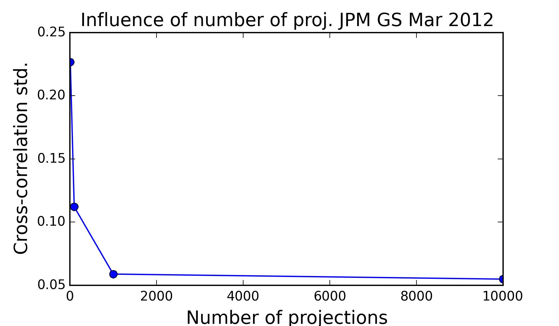
In order to guide practitioners in their choice of the number of Fourier basis elements to project onto, we conduct a numerical experiment on actual data. We compute an empirical standard deviation of the daily cross-correlogram obtained in January 2012 (19 days) for JPM (JP Morgan Chase) and GS (Goldman Sachs) with , , and projections. Figures 6 and 8 show that, as expected, the variance decreases linearly with the number of projections and we can obtain reliable estimates with projections.
 |
 |
 |
 |
5.5 Studying causality at scale
A primary goal of this work is to enable practical scalable causal inference for time series analysis. To evaluate scalability in a real-world setting in which , we assess the relation between AAPL and MSFT over the course of months. In contrast to our earlier experiments (shown in Figure 5), we no longer average daily cross-correlograms in and therefore only leverage concentration in the inverse Fourier transform step of the procedure. With only projections for observations per time series, the results we obtain on Figure 7 reveals the causal relation between AAPL, AAPL-LAG, IBM and MSFT consistently with Figure 5.
Scalability: In order to assess the scalability of the algorithm in a situation where communication is a major bottleneck, we run the experiment with Apache Spark on Amazon Web Services EC2 machines of type r3.2xlarge. In Figure 8 we show that even with a large number of projections () the communication burden is still low enough to achieve speed-up proportional to the number of machines used.
 |
 |
6 Conclusion
Time series analysis via the frequency domain presents several presents unique opportunities in terms of providing consistent causal estimates and scaling on distributed systems. We proposed a communication avoiding method to analyze causality which does not require any sorting or joining of data, works naturally with irregular timestamps without creating spurious causal estimates and makes the erasure of Long-Range dependencies embarrassingly parallel. Our approach is based on Fourier transforms as compression operators that do not modify the second order properties of stochastic processes. Applying an inverse Fourier transform to the resulting estimated spectra enables exploration of dependencies in the time domain. With the resulting consistent cross-correlogram, one can compute Lead-Lag ratios and characteristic delays between processes thereby infer linear causal structure. We show that projecting onto Fourier basis elements is sufficient to study stock market pair causality with tens of millions of high frequency recordings, thereby providing insightful analytics in a generic and scalable manner.
Acknowledgments: The authors would like to thank Prof. David R. Brillinger for his advice on the theoretical aspects of the method we presented. This material is based upon work supported by the National Aeronautics and Space Administration under Prime Contract Number NAS2-03144 awarded to the University of California, Santa Cruz, University Affiliated Research Center. This research is supported in part by NSF CISE Expeditions Award CCF-1139158, DOE Award SN10040 DE-SC0012463, and DARPA XData Award FA8750-12-2-0331, and gifts from Amazon Web Services, Google, IBM, SAP, The Thomas and Stacey Siebel Foundation, Adatao, Adobe, Apple Inc., Blue Goji, Bosch, Cisco, Cray, Cloudera, Ericsson, Facebook, Fujitsu, Guavus, HP, Huawei, Intel, Microsoft, Pivotal, Samsung, Schlumberger, Splunk, State Farm, Virdata and VMware.
References
- [1] P. Doukhan, G. Oppenheim, and M. S. Taqqu, Theory and applications of long-range dependence. Springer Science & Business Media, 2003.
- [2] C. W. Granger, “Causality, cointegration, and control,” Journal of Economic Dynamics and Control, vol. 12, no. 2, pp. 551–559, 1988.
- [3] F. Abergel, J.-P. Bouchaud, T. Foucault, C.-A. Lehalle, and M. Rosenbaum, Market microstructure: confronting many viewpoints. John Wiley & Sons, 2012.
- [4] R. S. Tsay, Analysis of financial time series. John Wiley & Sons, 2005, vol. 543.
- [5] M. Mudelsee, Climate time series analysis. Springer, 2013.
- [6] P. Shang, X. Li, and S. Kamae, “Chaotic analysis of traffic time series,” Chaos, Solitons & Fractals, vol. 25, no. 1, pp. 121–128, 2005.
- [7] I. Karatzas and S. Shreve, Brownian motion and stochastic calculus. Springer Science & Business Media, 2012, vol. 113.
- [8] N. Huth and F. Abergel, “High frequency lead/lag relationships - empirical facts,” Journal of Empirical Finance, vol. 26, pp. 41–58, 2014.
- [9] C. W. Granger, “Investigating causal relations by econometric models and cross-spectral methods,” Econometrica: Journal of the Econometric Society, pp. 424–438, 1969.
- [10] E. Parzen, Time Series Analysis of Irregularly Observed Data: Proceedings of a Symposium Held at Texas A & M University, College Station, Texas February 10–13, 1983. Springer Science & Business Media, 2012, vol. 25.
- [11] D. R. Brillinger, Time series: data analysis and theory. Siam, 1981, vol. 36.
- [12] N. Wiener, Extrapolation, interpolation, and smoothing of stationary time series. MIT press Cambridge, MA, 1949, vol. 2.
- [13] M. Friedman, “The interpolation of time series by related series,” Journal of the American Statistical Association, vol. 57, no. 300, pp. 729–757, 1962.
- [14] P. S. Linsay, “An efficient method of forecasting chaotic time series using linear interpolation,” Physics Letters A, vol. 153, no. 6, pp. 353–356, 1991.
- [15] P. J. Brockwell and R. A. Davis, Time Series: Theory and Methods. New York, NY, USA: Springer-Verlag New York, Inc., 1986.
- [16] T. Hayashi, N. Yoshida et al., “On covariance estimation of non-synchronously observed diffusion processes,” Bernoulli, vol. 11, no. 2, pp. 359–379, 2005.
- [17] M. Hoffmann, M. Rosenbaum, N. Yoshida et al., “Estimation of the lead-lag parameter from non-synchronous data,” Bernoulli, vol. 19, no. 2, pp. 426–461, 2013.
- [18] P. Flandrin, “On the spectrum of fractional brownian motions,” Information Theory, IEEE Transactions on, vol. 35, no. 1, pp. 197–199, 1989.
- [19] J. D. Scargle, “Studies in astronomical time series analysis. ii-statistical aspects of spectral analysis of unevenly spaced data,” The Astrophysical Journal, vol. 263, pp. 835–853, 1982.
- [20] N. R. Lomb, “Least-squares frequency analysis of unequally spaced data,” Astrophysics and space science, vol. 39, no. 2, pp. 447–462, 1976.
- [21] W. Palma, Long-memory time series: theory and methods. John Wiley & Sons, 2007, vol. 662.
- [22] D. B. Percival and A. T. Walden, Wavelet methods for time series analysis. Cambridge university press, 2006, vol. 4.
- [23] D. Peleg, “Distributed computing,” SIAM Monographs on discrete mathematics and applications, vol. 5, 2000.
- [24] V. Kumar, A. Grama, A. Gupta, and G. Karypis, Introduction to parallel computing: design and analysis of algorithms. Benjamin/Cummings Redwood City, CA, 1994, vol. 400.
- [25] F. Belletti, E. Sparks, M. Franklin, and A. M. Bayen, “Embarrassingly parallel time series analysis for large scale weak memory systems,” arXiv preprint arXiv:1511.06493, 2015.