Automated Clustering and Program Repair for Introductory Programming AssignmentsNote: Supported by the Austrian National Research Network S11403-N23 (RiSE) of the Austrian Science Fund (FWF).
Abstract.
Providing feedback on programming assignments is a tedious task for the instructor, and even impossible in large Massive Open Online Courses with thousands of students. Previous research has suggested that program repair techniques can be used to generate feedback in programming education. In this paper, we present a novel fully automated program repair algorithm for introductory programming assignments. The key idea of the technique, which enables automation and scalability, is to use the existing correct student solutions to repair the incorrect attempts. We evaluate the approach in two experiments: (I) We evaluate the number, size and quality of the generated repairs on 4,293 incorrect student attempts from an existing MOOC. We find that our approach can repair 97% of student attempts, while 81% of those are small repairs of good quality. (II) We conduct a preliminary user study on performance and repair usefulness in an interactive teaching setting. We obtain promising initial results (the average usefulness grade 3.4 on a scale from 1 to 5), and conclude that our approach can be used in an interactive setting.
Keywords:
programming education, MOOC, dynamic analysis, program repair, clustering
1. Introduction
Providing feedback on programming assignments is an integral part of a class on introductory programming and requires substantial effort by the teaching personnel. This problem has become even more pressing with the increasing demand for programming education, which universities are unable to meet (it is predicted that in the US by 2020 there will be one million more programming jobs than students (gee, [n. d.])). This has given rise to several Massive Open Online Courses (MOOCs) that teach introductory programming (Masters, 2011); the biggest challenge in such a setting is scaling personalized feedback to a large number of students.
The most common approach to feedback generation is to present the student with a failing test case; either generated automatically using test input generation tools (Tillmann et al., 2013) or selected from a comprehensive collection of representative test inputs provided by the instructor. This is useful feedback, especially since it mimics the setting of how programmers debug their code. However, this is not sufficient, especially for students in an introductory programming class, who are looking for more guided feedback to make progress towards a correct solution.
A more guided feedback can be generated from modifications that make a student’s program correct, using a program repair technique as pioneered by the AutoGrader tool (Singh et al., 2013). Generating feedback from program repair is an active area of research: One line of work focuses on improving the technical capabilites of program repair in introductory education (Rolim et al., 2017; Rivers and Koedinger, 2017; D’Antoni et al., 2016), while another line of research focuses on pedagogical questions such as how to best provide repair-based feedback to the students (Head et al., 2017; Suzuki et al., 2017). In this paper we propose a new completely automated approach for repairing introductory programming assignments, while sidelining the pedagogical questions for future work.
Our approach
The key idea of our approach is to use the wisdom of the crowd: we use the existing correct student solutions to repair the new incorrect student attempts11 1 We distinguish correct and incorrect attempts by running them on a set of inputs, and comparing their output to the expected output. This is the standard way of assessing correctness of student attempts in most introductory programming classes.. We exploit the fact that MOOC courses already have tens of thousands of existing student attempts; this was already noticed by Drummond et al. (2014).
Fig. 1 gives a high-level overview of our approach: (A) For a given programming assignment, we automatically cluster the correct student solutions (A-F in the figure), based on a notion of dynamic equivalence (see §2.1 for an overview and §4 for details). (B) Given an incorrect student attempt (G in the figure) we run the repair algorithm against all clusters, and then select a minimal repair ( in the figure) from the generated repair candidates (- in the figure). The repair algorithm uses expressions from multiple correct solutions to generate a repair (see §2.2 for an overview and §5 for details).
Intuitively, our clustering algorithm groups together similar correct solutions. Our repair algorithm can be seen as a generalization of the clustering approach of correct solutions to incorrect attempts. The key motivation behind this approach is as follows: to help the student, with an incorrect attempt, our approach finds the set of most similar correct solutions, written by other students, and generates the smallest modifications that get the student to a correct solution.
| ⬇ 1 def computeDeriv(poly): 2 result = [] 3 for e in range(1, len(poly)): 4 result.append(float(poly[e]*e)) 5 if result == []: 6 return [0.0] 7 else: 8 return result | ⬇ 1 def computeDeriv(poly): 2 deriv = [] 3 for i in xrange(1,len(poly)): 4 deriv+=[float(i)*poly[i]] 5 6 if len(deriv)==0: 7 return [0.0] 8 return deriv |
1.
result += [float(poly[e]*e),]
2.
if(e==0): result.append(0.0)
else: result.append(float(poly[e]*e)) 3. result.append(1.0*poly[e]*e) 4. result.append(float(e*poly[e])) 5. result += [e*poly[e]] |
1.
if(len(result)==0):
return [0.0] else: return result 2. if(len(result)>0): return result else: return [0.0] 3. return result or [0.0] |
| (a) Correct attempt C1. | (b) Correct attempt C2. | (c) Different expressions for . | (d) Different expressions for the return statement. |
| ⬇ 1 def computeDeriv(poly): 2 new = [] 3 for i in xrange(1,len(poly)): 4 new.append( 5 float(i*poly[i])) 6 if new==[]: 7 return 0.0 8 return new | ⬇ 1 def computeDeriv(poly): 2 result = [] 3 for i in range(len(poly)): 4 result[i]=float((i)*poly[i]) 5 return result | 1. In return statement at line 7, change 0.0 to [0.0]. |
1.
In iterator expression at line 3, change range(len(poly)) to
range(1, len(poly)). 2. In assignment at line 4, change result[i]=float(i*poly[i]) to result.append(float(i*poly[i])). 3. In return statement at line 5, change result to result or [0.0]. |
| (e) Incorrect attempt I1. | (f) Incorrect attempt I2. | (g) Repair for I1. | (h) Repair for I2. |
We have implemented the proposed approach in a tool called Clara and evaluated it in two experiments:
(I) On 12,973 correct and 4,293 incorrect (total 17,266) student attempts from an MITx MOOC, written in Python, we evaluate the number, size and quality of the generated repairs. Clara is able to repair 97% of student attempts, in 3.2s on average; we study the quality of the generated repairs by manual inspection and find that 81% of the generated repairs are of good-quality and the size of the generated repair matches the size of the required changes to the student’s program. Additionally, we compare AutoGrader and Clara, on the same MOOC data.
(II) We performed a preliminary user study about the performance and usefulness of Clara’s repairs in an interactive teaching setting. The study consisted of 52 participants who were asked to solve 6 programming assignments in C. The participants judged the usefulness of the generated repair-based feedback by 3.4 in average on a scale from 1 to 5.
Our experimental results demonstrate that Clara can, completely automatically, generate repairs of high quality, for a large number of incorrect student attempts in an interactive teaching setting for introductory programming problems.
This paper makes the following contributions:
- •
We propose an algorithm to automatically cluster correct student solutions based on a dynamic program analysis.
- •
We propose a completely automated algorithm for program repair of incorrect student attempts that leverages the wisdom of the crowd in a novel way.
- •
We evaluate our approach on a large MOOC dataset and show that Clara can repair almost all the programs while generating repairs of high quality.
- •
We find in a real-time user study that Clara is sufficiently fast to be used in an interactive teaching setting and obtain promising preliminary results from the participants of the user study on the usefulness of the generated feedback.
Differences to our earlier Technical Report. Our approach first appeared as a technical report22 2 https://arxiv.org/abs/1603.03165v1, together with a publicly available implementation33 3 https://github.com/iradicek/clara. While our core ideas are the same as in the technical report, we since have made several improvements of which we state here the two most important: (1) The repair algorithm uses expressions from different correct solutions in a cluster, as opposed to using only a single correct solution from a cluster. (2) We conducted a user study and added an extensive manual investigation of the generated repairs to the experimental evaluation.
Structure of the paper. In §2 we present an overview of our approach, in §3 we describe a simple imperative language, used for formalizing the notions of matching and clustering in §4 and the repair procedure in §5. We discuss our implementation and the experimental evaluation in §6, overview the related work in §7, discuss limitations and directions for future work in §8, and conclude in §9.
2. Overview
We discuss the high-level ideas of our approach on the student attempts to the assignment derivatives: “Compute and return the derivative of a polynomial function (represented as a list of floating point coefficients). If the derivative is 0, return [0.0].” Fig. 2 (a), (b), (e) and (f) show four student attempts to the above programming assignment: C1 and C2 are functionally correct, while I1 and I2 are incorrect.
2.1. Clustering of Correct Student Solutions
The goal of clustering is two-fold. (1) Scalability: elimination of dynamically equivalent correct solutions that the repair algorithm would otherwise consider separately. (2) Diversity of repairs: mining of dynamically equivalent, but syntactically different expressions from the same cluster, which are used to repair incorrect student attempts. We discuss the notion of dynamic equivalence next.
Matching
The clusters in our approach are the equivalence classes of a matching relation. We say that two programs and match, written , when: (1) they have the same control-flow (see the discussion below), and (2) there is a total bijective relation between the variables of and , such that related variables take the same values, in the same order, during the program execution on the same inputs. This is inspired by the notion of a simulation relation (Milner, 1971), adapted for a dynamic program analysis: whereas a simulation relation establishes that a program produces exactly the same values as program at corresponding program locations for all inputs, we are interested only in a fixed finite set of inputs. Therefore, we also call this notion dynamic equivalence, to stress that we use dynamic program analysis.
Control-flow
Our algorithms consider two control-flows the same if they have the same looping structure. That is, any loop-free sequence of code is treated as a single block; in particular, blocks can include (nested) if-then-else statements without loops (similar to Beyer et al. (2009)). We point out that we could have picked a different granularity of control-flow; e.g., to treat only straight line of code (without branching) as a block. We have picked this granularity because it enables matching of programs that have different branching-structure, and as a result our algorithm is able to generate repairs that involve missing if-then-else statements.
Example. Programs C1 and C2, from Fig. 2 (a) and (b), match, because: (1) they have the same control-flow since there is only a single loop in both programs; (2) there is the bijective variable relation , where variables ? and are special variables denoting the loop condition and the return value, which we need to make the control-flow and the return values explicit. For example, on the input , the variable , takes the value before the loop, the sequence of values inside the loop, and the value after the loop. Exactly the same values are taken by the variable ; and similarly for all the other variables. Therefore, C1 and C2 belong to the same cluster, which we denote by . For the further discussion, we need to fix one correct solution as a cluster representative; we pick C1, although it is irrelevant which program from the cluster we pick.
Although the expressions in the assignments to variables and generate the same values (i.e., they match or they are dynamically equivalent), the assignment expressions inside the loops are syntactically quite different; we state the expressions in terms of the variables of the cluster representative C1:
- •
append(result, float(poly[e]*e)) in C1, and
- •
result + [float(e)*poly[e]] in C2, where
the second expression has been obtained by replacing the variables from C2 with variables from C1 using the variable relation (e.g., we have replaced with , because ). In our benchmark we found 15 syntactically different, but dynamically equivalent, ways to write expressions for the assignment to , and 6 different ways to write the return expression (observing only different ASTs, and ignoring formatting differences). Some of these examples are shown in Fig. 2 (c) and (d), respectively. As we discuss in the next section, these different expressions are used by our repair algorithm.
2.2. Repair of Incorrect Student Attempts

Our repair algorithm takes an incorrect student attempt (which we call an implementation) and a cluster (of correct programs), and returns a repair; a repair modifies the implementation such that the repaired implementation and the cluster representative match. The top-level repair procedure takes an implementation and runs the repair algorithm on each cluster separately. Each repair has a certain cost w.r.t. some cost metric. In this paper we use syntactic distance. Finally, the repair with the minimal cost is chosen.
Fig. 2 (e) and (f) shows two incorrect programs, I1 and I2, and the generated repairs in (g) and (h), respectively. These repairs were generated using cluster , with its representative C1. Our algorithm also considered other cluster besides (which are not discussed here), but found the smallest repair using . In the rest of this section we discuss the repair algorithm on a single cluster.
Our algorithm generates repairs in two steps, which we discuss in more detail next: (1) The algorithm generates a set of local repairs for each implementation variable (its assigned expression). (2) Using constraint-optimization techniques, the algorithm selects a consistent subset of the local repairs with the smallest cost. The high-level overview of the algorithm is given in Fig. 3.
Local Repairs
A local repair ensures that an implementation expression , either modified or unmodified, matches a corresponding cluster representative expression . To establish that the expressions match, we need a variable relation that translates implementation variables to cluster variables, so that the expressions range over the same variables. We point out that for expression matching it is sufficient to consider partial variable relations that relate variables of the expressions, as opposed to total variable relations that relate all program variables, which we considered above for program matching.
Let be an implementation variable, with expression assigned to it at some program location. We say that is a local repair for , if the expressions and match, where is a partial variable relation that establishes the matching. In this case the implementation expression is modified to the repaired expression . We discuss below how the algorithm generates the repaired expression . We say that is a local repair for , if the expressions and match, where is a partial variable relation that establishes the matching. In this case the implementation expression remains unmodified.
We illustrate the notion of local repairs on I1 with regard to the cluster representative C1:
- 1.
is a local repair for before the loop, where , since the expressions of and match (i.e., they take the same values).
- 2.
is a local repair for after the loop, where , since then the return expressions match. - 3.
is a local repair for after the loop, where , since then the return expressions match.
The algorithm generates a set of such local repairs for each variable and each program location in the implementation.
Finding a repair
A (whole program) repair is a consistent subset of the generated local repairs, such that there is exactly one local repair for each variable and each program location in the implementation. A set of local repairs is consistent when all partial variable relations in the local repairs are subsets of some total variable relation. For example, local repairs (1) and (3) from above are inconsistent, since we have and , and hence there is no total variable relation that is consistent with both and . On the other hand, local repairs (1) and (2) are consistent, since there is a total variable relation consistent both with and : .
There are many choices for a whole program repair, that is, choices for a consistent subset of the generated local repairs; however, we are interested in one that has the smallest cost. Our algorithm finds such a repair using constraint-optimization techniques.
Generating the set of potential local repairs
The repair algorithm takes expressions from the different correct solutions in order to generate the set of potential local repairs ( discussed above). The algorithm translates these expressions to range over the implementation variables, using a partial variable relation. Since each cluster expression matches a corresponding cluster representative expression (recall the discussion in the previous sub-section), this partial variable relation ensures that matches a corresponding cluster representative expression (i.e., that it is a correct repair).
For example, the generated repair for I2, shown in Fig. 2 (h), combines the following expressions from the cluster:
- •
The first modification is generated using the expression range(1, len(poly)) from C1, at line 3, using the partial variable relation .
- •
The second modification is generated using the expression (4.) from Fig. 2 (c), using the partial variable relation .
- •
The third modification is generated using the expression (3.) from Fig. 2 (d), using the partial variable relation .
3. Program Model
In this section we define a program model that captures key aspects of imperative languages (e.g., C, Python). This model allows us to formalize our notions of program matching and program repair.
Definition 3.1 (Expressions).
Let be a set of variables, a set of constants, and a set of operations. The set of expressions is built from variables, constants and operations in the usual way. We fix a set of special variables . We assume that includes at least the variable ?, which we will use to model conditions, and the variable , which we will use to model return values.
Def. 3.1 can be instantiated by a concrete programming language. For example, for the C language, can be chosen to be the set of all C constants (e.g., integer, float), and can be chosen to be the set of unary and binary C operations as well as library functions. The special variables are assumed to not appear in the original program text, and are only used for modelling purposes.
Definition 3.2 (Program).
A program is a tuple, where is a (finite) set of locations, is the initial location, is a (finite) set of program variables, is the variable update function that assigns an expression to every location-variable pair, and is the successor function, which either returns a successor location in or the special value (we assume ). We drop the subscript when it is clear from the context.
We point the reader to the discussion around the semantics below for an intuitive explanation of the program model.
Definition 3.3 (Computation domain, Memory).
We assume some (possibly infinite) set of values, which we call the computation domain, containing at least the following values: (1) true (bool true); (2) false (bool false); and (3) (undefined).
Let be a set of variables. A memory is a mapping from program variables to values, where the set denotes the primed version of the variables in ; let denote the set of all memories over variables .
Intuitively, the primed variables are used to denote the variable values after a statement has been executed (see the discussion around the semantics below).
Definition 3.4 (Evaluation).
A function is an expression evaluation function, where denotes that , on a memory , evaluates to a value .
The function is defined by a concrete programming language. The function returns the undefined value () when an error occurs during the execution of an actual program.
Definition 3.5 (Program Semantics).
Let be a program. A sequence of location-memory pairs is called a trace. Given some (input) memory , we write if: (1) ; (2) for all ; (3) (a) , and (b) , and (c) , for all and ; and (4) , for any .
For some trace element and a variable , denotes the value of before the location is evaluated (the old value of at ), and denotes the value of after the location is evaluated (the new value of at ). The definition of then says:
- (1)
The first location of the trace is the initial location .
- (2)
The old values of the variables at the initial location are defined by the input memory .
- (3a)
The new value of variable at location is determined by the semantic function evaluated on the expression .
- (3b)
The old value of variable at location is equal to the new value at location .
- (3c)
The next location in a trace is determined by the successor function for the current location and the new value of ? at (i.e., ).
- (4)
The successor of the last location, , for any Boolean , is the end location .
Modelling of if-then-else statements
In our implementation we model if-then-else statements differently, according to when they contain loops and when they are loop-free (as mentioned in §2.1). In the former case, the branching is modelled, as usual, directly in the control-flow. In the latter case, (loop-free) statements are (recursively) converted to ite expressions that behave like a C ternary operator (as in the example that follows).
Example. We now show how a concrete program (C1 from Fig. 2 (a)) is represented in our model. The set of locations is , where is the location before the loop, and the initial location, is the location of the loop condition, is the loop body, and is the location after the loop. The successor function is given by , , , , and . Note that for non-branching locations the successor functions points to the same location for both true and false.
The set of variables is , where is used to model Python’s for-loop iterator. An iterator is a sequence whose elements are assigned, one by one, to some variable ( in this example) in each loop iteration. The expression labeling function is given by:
- •
,
- •
,
- •
,
- •
,
- •
,
- •
,
- •
.
For any variable that is unassigned at some location we set , i.e., the variable remains unchanged.
Finally, we state the trace when C1 is executed on .
We state only defined variables that change from one trace element to the next.
Otherwise, we assume the values remain the same or are undefined () (if no previous value existed).
,
,
,
,
,
,
.
4. Matching and Clustering
In this section we formally define our notion of matching.
Informally, two programs match, if (1) the programs have the same control-flow (i.e., the same looping structure), and (2) the corresponding variables in the programs take the same values in the same order. For the following discussion we fix two programs, and .
Definition 4.1 (Program Structure).
Programs and have the same control-flow if there exists a bijective function, called structural matching, , s.t., for all and , .
We remind the reader, as discussed in §2 and §3, that we encode any loop-free program part as single control-flow location; as a result we compare only the looping structure of two programs.
We note that both our matching and repair algorithms require the existence of a structural matching between programs. Therefore, in the rest of the paper we assume that such a exists between any two programs that we discuss, and assume that and , since they can be always converted back and forth using . Next, we state two definitions that will be useful later on.
Definition 4.2 (Variables of expression).
Let be some expression, by we denote the set of variables used in the expresison . We also say that ranges over .
Definition 4.3 (Variable substitution).
Let be some function that maps variables to variables . Given an expression over variables , i.e., , by we denote the expression, which we obtain from , by substituting with for all . Note that .
Given a memory , over variables , we define , that is, the memory where is substituted with , for all . We lift substitution to a trace , by applying it to the each element: .
In the rest of the paper we call a bijective function , between two sets of variables and , a total variable relation between and . Next we give a formal definition of matching between two programs. Afterwards, we give a formal definition of matching between two expressions. The definitions involve execution of the programs on a set of inputs.
Definition 4.4 (Program Matching).
Let be a set of inputs, and let and be sets of traces obtained by executing and on , respectively.
We say that and match over a set of inputs , denoted by , if there exists a total variable relation , such that , for all inputs . We call a matching witness.
Intuitively, a matching witness defines a way of translating to range over variables , such that and translated with produce the same traces.
Given a set of inputs , is an equivalence relation on a set of programs : the identity relation on program variables gives a matching witness for reflexivity, the inverse of some total variable relation gives a matching witness for symmetry, and the composition of some total variables relations gives a matching witness for transitivity.
The algorithm for finding is given in Fig. 4: given two programs and and a set of inputs , it returns a matching witness , if one exists. The algorithm first executes both programs on the inputs (lines 3 and 4), and then for each variable finds a set of variables from that take the same values during execution, thus defining a set of potential matches (lines 5-10); here , denotes a projection of values of variable from a trace , that is: . The matching witness is then a bijective mapping , if one exists (line 11); can be found in by constructing a maximum bipartite matching in the bipartite graph defined by . We note that this problem can be solved in polynomial time, w.r.t. the number of the edges and vertices in (e.g.,Uno (1997)).
Definition 4.5 (Expression matching).
Let be a set of traces over variables , and let and be two expressions over variables , at some location .
We say that and match over a set of traces , denoted , if , for all where , and all .
Expression matching says that two expressions produce the same values, when considering the memories at location , in a set of traces . In the following lemma we state that expression matching is equivalent to program matching; this lemma will be useful for our repair algorithm, which we will state in the next section.
Lemma 4.6 (Matching Equivalence).
Let be a set of inputs, and let be a set of traces obtained by executing on . We have the following equivalence: witnessed by , if and only if, , for all , where , , and .
Proof.
“”: Directly from the definitions. “”: By induction on the length of the trace for some . ∎
Clustering
We define clusters as the equivalence classes of . For the purpose of matching and repair we pick an arbitrary class representative from the class and collect expressions from all programs in the same cluster:
Definition 4.7 (Cluster).
Let be a set of (correct) programs. A cluster is an equivalence class of . Given some cluster , we fix some arbitrary class representative .
We define the set of cluster expressions for a pair : iff there is some witnessed by such that , and .
Note that it is irrelevant which program from is chosen as cluster representative ; we just need to fix some program in order to be able to define the expressions over a common set of variables . We note that by definition the sets of expressions have the following property: for all we have that is, expressions and match.
Example. In §2.1 we discussed why the solutions C1 and C2 match; therefore these two solutions belong to the same cluster, which we denote here by , and chose C1 as its representative . Also, in Fig. 2 (c) and (d) we gave examples of different equivalent expressions of assignment to the variable inside the loop body and the return statement after the loop, respectively. To be more precise, these were examples of sets and , respectively.
5. Repair Algorithm
In the previous section we defined the notion of a matching between two programs. In this section we consider an implementation and a cluster (with its representative ) between which there is no matching. We assume that and have the same control-flow. The goal is to repair ; that is, to modify minimally, w.r.t. some notion of cost, such that the repaired program matches the cluster. More precisely, the repair algorithm searches for a program , such that , and should be syntactically close to . Therefore, our repair algorithm can be seen as a generalization of clustering to incorrect programs.
We first define a version of the repair algorithm that does not change the set of variables, i.e., . Below we extend this algorithm to include changes of variables, i.e., we allow . In both cases the control-flow of remains the same.
For the following discussion we fix some set of inputs . Let be the set of traces of cluster representative for the inputs .
As we discussed in the previous section, two programs match if all of their corresponding expressions match (see Lemma 4.6). Therefore the key idea of our repair algorithm is to consider a set of local repairs that modify individual implementation expressions. We first discuss local repairs; later on we will discuss how to combine local repairs into a full program repair.
Local repairs are defined with regard to partial variable relations. It is enough to consider partial variable relations (as opposed to the total variable relations needed for matchings) because these relations only need to be defined for the expressions that need to be repaired.
Definition 5.1 (Local Repair).
Let be a location-variable pair from , and let be the corresponding expression. Further, let be a partial variable relation such that , let be the related cluster representative variable, and let be the corresponding expression.
A pair , where is an expression over implementation variables , is a local repair for when and . A pair is a local repair for when and .
We define the cost of a local repair as and the cost of a local repair as .
We comment on the definition of a local repair. Let be a location-variable pair from , let be the corresponding expression, and let be a local repair for some . In case , the expression matches the corresponding expression of the cluster representative under the partial variable mapping ; this repair has cost zero because the expression is not modified. In case , the expression constitutes a modification of that matches the corresponding expression of the cluster representative under the partial variable mapping ; this repair has some cost . In our implementation we define to be the tree edit distance (Tai, 1979; Zhang and Shasha, 1989) between the abstract syntax trees (ASTs) of the expressions and .
Example. We remind the reader that in §2.2 we discussed three examples of local repairs for I1 (Fig. 2). Formally, example (1) is a local repair for , while (2) and (3) are local repairs for . Next we state how to combine local repairs into a full program repair.
Definition 5.2 (Repair).
Let be a function that assigns to each pair a local repair for . We say that is consistent, if there exists a total variable relation , such that , for all . A consistent is called a repair. We define the cost of as the sum of the costs of all local repairs: .
A repair defines a repaired implementation , where if , and if , for all .
Theorem 5.3 (Soundness of Repairs).
.
Proof.
(sketch) From the definition of , we have , for all , where , and . Then it follows from Lemma 4.6 that . ∎
In the above definition we use notation when or is not important in ; similarly we use and when is not important in .
Example. The repair for example I1 (Fig. 2) corresponds to the total variable relation . The repair includes local repairs (1) and (2) from the previous examples, where only (2) has cost (see the repair in Fig. 2 (g)).
Next we discuss the algorithm for finding a repair.
The repair algorithm
The algorithm is given in Fig. 5: given a cluster , an implementation , and a set of inputs , it returns a repair . The algorithm has two main parts: First, the algorithm constructs a set of possible local repairs; we define and discuss the possible local repairs below. Second, the algorithm searches for a consistent subset of the possible local repairs, which has minimal cost; this search corresponds to solving a constraint-optimization system.
Definition 5.4 (Set of possible local repairs).
For all , we define the set of possible local repairs as: (1) , if ; and (2) , if , where and .
The set of possible local repairs includes all expressions from the cluster , translated by some partial variable relation in order to range over implementation variables. It also includes if matches under partial variable mapping . Next we describe how the algorithm constructs the set (at lines 4-14).
For the following discussion we fix a pair (corresponding to line 4), and some (corresponding to line 7); we set and . Possible local repairs for are constructed in two steps: In the first step, the algorithm checks if there are partial variable relations s.t. (at line 9), and in that case adds a pair to (at line 11). In the second step, the algorithm iterates over all cluster expressions (at line 12), and all partial variable relations (at line 13), and then adds a pair to (at line 14). We note that , and thus is a possible local repair as in Def. 5.4.
We remark that in both steps, the algorithm iterates over all possible variable relations . However, since relates only the variables of a single expression — usually a small subset of all program variables, this iteration is feasible.
Finding a repair with the smallest cost
Finally, the algorithm uses sub-routine FindRepair (at line 15) that, given a set of possible local repairs , finds a repair with smallest cost. FindRepair encodes this problem as a Zero-One Integer Linear Program (ILP), and then hands it to an off-the-shelf ILP solver. Next, we define the ILP problem, describe how we encode the problem of finding a repair as an ILP problem, and how we decode the ILP solution to a repair.
Definition 5.5 ((Zero-One) ILP).
An ILP problem, over variables , is defined by an objective function , and a set of linear (in)equalities , of the form . Where and . A solution to the ILP problem is a variable assignment , such that all (in)equalities hold, and the value of the objective functions is minimal (resp. maximal) for .
We encode the problem of finding a consistent subset of possible local repairs as an ILP problem with variables ; that is, one variable for each pair of variables , and one variable for each possible local repair . The set of constraints is defined as follows:
| (1) | ||||
| (2) | ||||
| (3) | ||||
| (4) | ||||
Intuitively, the constraints encode:
- (1)
Each is related to exactly one of .
- (2)
Each is related to exactly one of . Together (1) and (2) encode that there is a total variable relation .
- (3)
For each exactly one local repair is selected.
- (4)
Each selected local repair is consistent with , i.e., .
The objective function ensures that the sum of the costs of the selected local repairs is minimal.
Let be a solution of the ILP problem. We obtain the following total variable relation from : iff . For , where , we set .
Adding and Deleting Variables
The repair algorithm described so far does not change the set of variables, i.e., . However, since the repair algorithm constructs a bijective variable relation, this only works when the implementation and cluster representative have the same number of variables, i.e., . Hence, we extend the algorithm to also allow the addition and deletion of variables.
We extend total variable relations to relations . We relax the condition about being total and bijective: and can be related to multiple variables or none. When some variable is related to , that is , it denotes that a fresh variable is added to , in order to match . Conversely, when some variable is related to , that is , variable is deleted from , together with all its assignments.
Completeness of the algorithm
We point out that with this extension the repair algorithm is complete (assuming and have the same control-flow). This is because the repair algorithm can always generate a trivial repair: all variables are deleted, that is for all ; and a fresh variable is introduced for every variable , that is for all . Clearly, this trivial repair has high cost, and in practice it is very rarely generated, as witnessed by our experimental evaluation in the next section.
6. Implementation and Experiments
| Problem | LOC | AST size | # correct | # clusters | # incorrect | # repaired (% of # incorrect) | avg. (median) time in s | ||
|---|---|---|---|---|---|---|---|---|---|
| name | median | median | (% of # correct) | Clara | AutoGrader | Clara | AutoGrader | ||
| derivatives | () | () | () | s (s) | s (s) | ||||
| oddTuples | () | () | () | s (s) | s (s) | ||||
| polynomials | () | () | () | s (s) | s (s) | ||||
| Total | () | () | () | s (s) | s (s) | ||||
We now describe our implementation (§6.1) and an experimental evaluation, which consists of two parts: (I) an evaluation on MOOC data (§6.2), and (II) a user study about the usefulness of the generated repairs (§6.3). The evaluation was performed on a server with an AMD Opteron 6272 2.1GHz processor and 224 GB RAM.
6.1. Implementation
We implemented the proposed approach in the publicly available tool Clara44 4 https://github.com/iradicek/clara (for CLuster And RepAir). The tool currently supports programs in the programming languages C and Python, and consists of: (1) Parsers for C and Python that convert programs to our internal program representation; (2) Program and expression evaluation functions for C and Python, used in the matching and repair algorithms; (3) Matching algorithm; (4) Repair algorithm; (5) Simple feedback generation system. We use the lpsolve (lps, [n. d.]) ILP solver, and the zhang-shasha (zha, [n. d.]) tree-edit-distance algorithm.
Feedback generation
We have implemented a simple feedback generation system that generates the location and a textual description of the required modifications (similar to AutoGrader). Other types of feedback can be generated from the repair as well, and we briefly discuss it in §9.
6.2. MOOC Evaluation
Setup
In the first experiment we evaluate Clara on data from the MITx introductory programming MOOC (mit, [n. d.]), which is similar to the data used in evaluation of AutoGrader (Singh et al., 2013).
This data is stripped from all information about student identity, i.e., there are not even anonymous identifiers. To avoid the threat that a student’s attempt is repaired by her own future correct solution, we split the data into two sets. From the first (chronologically earlier) set we take only the correct solutions: these solutions are then clustered, and the obtained clusters are used during the repair of the incorrect attempts. From the second (chronologically later) set we take only the incorrect attempts: on these attempts we perform repair. We have split the data in ratio since then we have a large enough number (; see the discussion below) of correct solutions that our approach requires, while still having quite a large number () of incorrect attempts for the repair evaluation. We point out that this is precisely the setting that we envision our approach to be used in: a large number of existing correct solutions (e.g., from a previous offering of a course) are used to repair new incorrect student submissions.
Results
The evaluation summary is in Table 1; the descriptions of the problems are in the appendix §A. Clara automatically generates a repair for 97.44% of attempts. As expected, Clara can generate repairs in almost all the cases, since there is always the trivial repair of completely replacing the student implementation with some correct solution of the same control flow. Hence, it is mandatory to study the quality and size of the generated repairs. We evaluate the following questions in more detail: (1) What are the reasons when Clara fails? (2) Does Clara generate non-trivial repairs? (3) What is the quality and size of the generated repairs?
We discuss the results of this evaluation below, while further examples can be found in the appendix §B.
(1) Clara fails
Clara fails to generate repair in 110 cases: in 69 cases there are unsupported Python features (e.g., nested function definitions), in 35 cases there is no correct attempt with the same control-flow, and in 6 cases a numeric precision error occurs in the ILP solver. The only fundamental problem of our approach is the inability to generate repairs without matching control-flow; however, since this occurs very rarely, we leave the extension for a future work. Hence, we conclude that CLARA can repair almost all programs.

(2) Non-trivial repairs
Since a correct repair is also a trivial one that completely replaces a student’s attempt with a correct program, we measure how much a repair changes the student’s program. To measure this we examine the relative repair size: the tree-edit-distance of the repair divided by the size of the AST of the program. Intuitively, the tree-edit-distance tells us how many changes were made in a program, and normalization with the total number of AST nodes gives us the ratio of how much of the whole program changed. Note, however that this ratio can be , or even if the program is empty. Fig. 6 shows a histogram of relative repair sizes. We note that of all repairs have relative size , have and have ; the last column () is caused by completely empty student attempts. As an example, the two repairs in Fig. 2 (g) and (h), have relative sizes of and . We conclude that Clara in almost all cases generates a non-trivial repair that is not a replacement of the whole student’s program.
 |
 |
| (a) The number of modified expressions per repair. | (b) Distribution of the number of modified expressions per repair. |
(3) Repair quality and repair size
We inspected 100 randomly selected generated repairs, with the goal of evaluating their quality and size. Our approach of judging repair quality and size mirrors a human teacher helping a student: the teacher has to guess the student’s idea and use subjective judgment on what feedback to provide. We obtained the following results: (a) In 72 cases Clara generates the smallest, most natural repair; (b) In 9 cases the repair is almost the smallest, but involves an additional modification that is not required; (c) In 11 cases we determined the repair, although correct, to be different from the student’s idea; (d) In 8 cases it is not possible to determine the idea of the student’s attempt, although Clara generates some correct repair.
For the cases in (d), we found that program repair is not adequate and further research is needed to determine what kind of feedback is suitable when the student is far from any correct solution. For the cases in (c), the set of correct solutions does not contain any solution which is syntactically close to the student’s idea; we conjecture that Clara’s results in these cases can partially be improved by considering different cost functions which do not only take syntactic differences into account but also make use of semantic information (see the discussion in §9). However, in 81 cases (the sum of (a) and (b)), Clara generates good quality repairs. We conclude that Clara mostly produces good quality repairs.
Summary
Our large-scale experiment on the MOOC data-set shows that Clara can fully automatically repair almost all programs and the generated repairs are of high quality.
Clusters
Finally, we briefly discuss the correct solutions, since our approach depends on their existence. The quality of the generated repair should increase with the number of clusters, since then the algorithm can generate more diverse repairs. Thus, it is interesting to note that we experienced no performance issues with a large number of clusters; e.g., on derivatives, with 532 clusters, a repair is generated on average in 4.9s. This is because the repair algorithm processes multiple clusters in parallel. Nonetheless, clustering is important for repair quality, since it enables repairs that combine expressions taken from different correct solutions from the same cluster, which would be impossible without clustering. We found that (around ) repairs were generated using at least two different correct solutions, and (around ) were generated using at least three different correct solutions, in the same cluster.
6.2.1. Comparison with AutoGrader
While the setting of AutoGrader is different (a teacher has to provide an error model, while our approach is fully automated), the same high-level goal (finding a minimal repair for a student attempt to provide feedback) warrants an experimental comparison between the approaches.
Setup and Data
We were not able to obtain the data used in AutoGrader’s evaluation, which stems from an internal MIT course, because of privacy concerns regarding student data. Hence, we compare the tools on the same MITx introductory programming MOOC data, which we used in the paper for Clara evaluation. This dataset is similar to the dataset used in AutoGrader’s evaluation. AutoGrader’s authors provided us with an AutoGrader version that is optimized to scale to a MOOC, that is, it has a weaker error model than in the original AutoGrader’s publication (Singh et al., 2013). According to the authors, some error rewrite rules were intentionally omitted, since they are too slow for interactive online feedback generation.
Results
The evaluation summary is in Table 1. AutoGrader is able to generate a repair for 19.29% of attempts, using manually specified rewrite-rules, compared to 97.44% automatically generated repairs by Clara. (We note that AutoGrader is able to repair fewer attempts than reported in the original publication (Singh et al., 2013) due to the differences discussed in the previous paragraph.) As Clara can generate repairs in almost all the cases, these numbers are not meaningful on their own; the numbers are, however, meaningful in conjunction with our evaluation of the following questions: (1) How many repairs can one tool generate that other cannot, and what are the reasons when AutoGrader fails? (2) What are the sizes of repairs? (3) What is the quality of the generated repairs, in case both tools generate a repair?
We summarize the results of this evaluation below, while a more detailed discussion can be found in the appendix §B.
(1) Repair numbers
In all but one case, when Clara fails to generate a repair, AutoGrader also fails. Further, we manually inspected 100 randomly selected cases where AutoGrader fails, and determined that in 77 cases there is a fundamental problem with AutoGrader’s approach: The modifications require fresh variables, new statements or larger modifications, which are beyond AutoGrader’s capabilities. This shows that Clara can generate more complicated repairs than AutoGrader.
In the 100 cases we manually inspected we also determined that in 74 cases Clara generates good quality repairs, when AutoGrader fails.
(2) Repair sizes
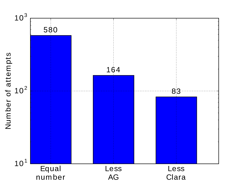
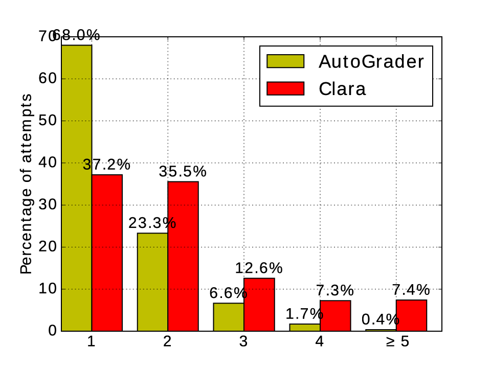
We do not report the relative repair size metric for AutoGrader, because we were not able to extract the repair size from its (textual) output. However, Fig. 7 (a) compares the relation of the number of modified expressions when both tools generate a repair. We note that the number of modified expressions is a weaker metric than the tree-edit-distance, however, we were only able to extract this metric for the repairs generated by AutoGrader. We conclude that AutoGrader produces smaller repair in around 10% of the cases.
Fig. 7 (b) also compares the overall (not just when both tools generate a repair) distribution of the number of changed expression per repair. We notice that most of AutoGrader’s repairs modify a single expression, and the percentage falls faster than in Clara’s case.
| Problem | LOC | # correct | # clusters | # incorr. | # feedback | # repair feedback | time (in s) | # grades | |
|---|---|---|---|---|---|---|---|---|---|
| median | (exist.+study) | (exist.+study) | (% of # incorr.) | (% of # feedback) | avg. | median | 1/2/3/4/5 | ||
| Fibonacci sequence | 12 | 512+84 | 70 + 17 (14.60%) | 572 | 539 (94.23%) | 440 (81.63%) | 10.44 | 8.51 | 1 / 7 / 9 / 16 / 13 |
| Special number | 15 | 358+59 | 39 + 3 (10.07%) | 121 | 109 (90.08%) | 94 (86.24%) | 3.77 | 2.38 | 2 / 3 / 8 / 9 / 13 |
| Reverse Difference | 17 | 342+46 | 48 + 8 (14.43%) | 103 | 77 (74.76%) | 68 (88.31%) | 4.39 | 3.07 | 4 / 4 / 5 / 3 / 5 |
| Factorial interval | 14 | 391+44 | 56 + 8 (14.71%) | 234 | 232 (99.15%) | 185 (79.74%) | 3.33 | 3.17 | 2 / 5 / 4 / 5 / 13 |
| Trapezoid | 14 | 281+41 | 36 + 15 (15.84%) | 143 | 129 (90.21%) | 121 (93.80%) | 7.55 | 4.82 | 7 / 5 / 7 / 7 / 5 |
| Rhombus | 21 | 264+38 | 73 + 22 (31.46%) | 525 | 417 (79.43%) | 192 (46.04%) | 9.16 | 5.35 | 6 / 9 / 6 / 5 / 3 |
(3) Repair quality
Finally, we manually inspected 100 randomly selected cases where both tools generate a repair. In 61 cases we found both tools to produce the same repair; in 19 cases different, although of the same quality; in 9 cases we consider AutoGrader to be better; in 5 cases we consider Clara to be better; and in 6 cases we found that AutoGrader generates an incorrect repair. We conclude that there is no notable difference between the tools when both tools generate a repair.
6.3. User Study on Usefulness
In the second experiment we performed a user study, evaluating Clara in real time. We were interested in the following questions: (1) How often and fast is feedback generated (performance)? (2) How useful is the generated repair-based feedback?
Setup
To answer these questions we developed a web interface for Clara and conducted a user study, which we advertised on programming forums, mailing lists, and social networks. Each participant was asked to solve six introductory C programming problems, for which the participants received feedback generated by Clara. There was one additional problem, not discussed here, that was almost solved, and whose purpose was to familiarize the participants with the interface. After solving a problem each participant was presented with the question: “How useful was the feedback provided on this problem?”, and could select a grade on the scale from 1 ("Not useful at all") to 5 ("Very useful"). Additionally, each participant could enter an additional textual comment for each generated feedback individually and at the end of solving a problem.
We also asked the participants to assess their programming experience with the question: “Your overall programming experience (your own, subjective, assessment)”, with choices on the scale from 1 (“Beginner”) to 5 (“Expert”).
The initial correct attempts were taken from an introductory programming course at IIT Kanpur, India. The course is taken by around 400 students of whom several have never written a program before. We selected problems from two weeks where students start solving more complicated problems using loops. Of the 16 problems assigned in these two weeks, we picked those 6 that were sufficiently different.
Results
Table 2 shows the summary of the results; detailed descriptions of all problems are available in the appendix §A. The columns # correct and # clusters show the number of correct attempts and clusters obtained from: (a) the existing ESC 101 data (exist. in the table), and (b) during the case study from participants’ correct attempts (study in the table). We plan to make the complete data, with all attempts, grades and textual comments publicly available.
Performance of Clara
Feedback was generated for 1503 (88.52%) of incorrect attempts. In the following we discuss the 3 reasons why feedback could not be generated: (1) In 57 cases there was a bug in Clara, which we have fixed after the experiment finished. Then we confirmed that in all 57 cases the program is correctly repaired and feedback is generated (note that this bug was only present in this real-time experiment, i.e., it did not impact the experiment described in the previous section); (2) In 43 cases a timeout occurred (set to 60s); (3) In 95 cases a program contained an unsupported C construct, or there was a syntactic compilation error that was not handled by the web interface (Clara currently provides no feedback on programs that cannot be even parsed). Further, the average time to generate feedback was 8 seconds. These results show that Clara provides feedback on a large percentage of attempts in real time.
Feedback usefulness
The results are based on 191 grades given by 52 participants. Note that problems have a different number of grades. This is because we asked for a grade only when feedback was successfully generated (as noted above, in cases), and because some of the participants did not complete the study. The average grade over all problems is 3.4. This shows very promising preliminary results on the usefulness of Clara. However, we believe that these results can be further improved (see §9).
The participants declared their experience as follows: 22 as 5, 19 as 4, 9 as 3, 0 as 2, and 2 as 1. While these are useful preliminary results, a study with beginner programmers is an important future work.
Note. In the case of a very large repair ( in our study), we decided to show a generic feedback explaining a general strategy on how to solve the problem. This is because the feedback generated by such a large repair is usually not useful. We generated such a general strategy in 403 cases.
6.4. Threats to Validity
Program size
We have evaluated our approach on small to medium size programs typically found in introductory programming problems. The extension of our approach to larger programming problems, as found in more advanced courses, is left for future work. Focusing on small to medium size programs is in line with related work on automated feedback generation for introductory programming (e.g., D’Antoni et al. (2016), Singh et al. (2013), Head et al. (2017)). We stress that the state-of-the-art in teaching is manual feedback (as well as failing test cases); thus, automation, even for small to medium size programs, promises huge benefits. We also mention that our dataset contains larger and challenging attempts by students which use multiple functions, multiple and nested loops, and our approach is able to handle them.
The focus of our work differs from the related work on program repair (see §7 for a more detailed discussion). Our approach is specifically designed to perform well on small to medium size programs typically found in introductory programming problems, rather than the larger programs targeted in the literature on automated program repair. In particular, our approach addresses the challenges of (1) a high number of errors (education programs are expected to have higher error density (Singh et al., 2013)), (2) complex repairs, and (3) a runtime fast enough for use in an interactive teaching environment. These goals are often out of reach for program repair techniques. For example, the general purpose program repair techniques discussed in Goues et al. (2015) on the IntroClass benchmark, either repair a small number of defects (usually <50%) or take a long time (i.e., over one minute).
Unsoundness
Our approach guarantees only that repairs are correct over a given set of test cases. This is in accordance with the state-of-the-art in teaching, where testing is routinely used by course instructors to grade programming assignments and provide feedback (e.g., for ESC101 at IIT Kanpur, India (Das et al., 2016)). When we manually inspected the repairs for their correctness, we did not find any problems with soundness. We believe that this due to the fact that programming problems are small, human-designed problems that have comprehensive sets of test cases.
In contrast to our dynamic approach, one might think about a sound static approach based on symbolic execution and SMT solving. We decided for a dynamic analysis because symbolic execution can sometimes take a long time or even fail when constructs are not supported by an SMT solver. For example, reasoning about floating points and lists is difficult for SMT solvers. On the other hand, our method only executes given expressions on a set of inputs, so we can handle any expression, and our method is fast. Further, our evaluation showed our dynamic approach to be precise enough for the domain of introductory programming assignments. The investigation of a static verification of the results generated by our repair approach is an interesting direction for future work: one could take the generated repair expressions and verify that they indeed establish a simulation with the cluster against which the program was repaired.
7. Related Work
Automated Feedback Generation
Ihantola et al. (2010)
present a survey of
tools for the automatic assessment of programming exercises.
Pex4Fun (Tillmann et al., 2013) and its successor CodeHunt (Tillmann et al., 2014)
are browser-based, interactive platforms
where students solve programming assignments with hidden specifications, and
are presented with a list of automatically generated test cases.
LAURA (Adam and Laurent, 1980) heuristically applies program transformations to a student’s
program and compares it to a reference solution, while reporting mismatches
as potential errors (they could also be correct variations).
Apex (Kim et al., 2016) is a system that automatically generates error explanations
for bugs in assignments, while our work automatically clusters
solutions and generates repairs for incorrect attempts.
Trace analysis
Striewe and Goedicke (2011) have proposed presenting full program traces to the students, but the interpretation of the traces is left to the students. They have also suggested automatically comparing the student’s trace to that of a sample solution (Striewe and Goedicke, 2013). However, the approach misses a discussion of the situation when the student’s code enters an infinite loop, or has an error early in the program that influences the rest of the trace. The approach of Gulwani et al. (2014) uses a dynamic analysis based approach to find a strategy used by the student, and to generate feedback for performance aspects. However, the approach requires specifications manually provided by the teacher, written in a specially designed specification language, and it only matches specifications to correct attempts, i.e., it cannot provide feedback on incorrect attempts.
Program Classification in Education
CodeWebs (Nguyen et al., 2014) classifies different AST sub-trees in equivalence classes based on probabilistic reasoning and program execution on a set of inputs. The classification is used to build a search engine over ASTs to enable the instructor to search for similar attempts, and to provide feedback on some class of ASTs. OverCode (Glassman et al., 2014) is a visualization system that uses a lightweight static and dynamic analysis, together with manually provided rewrite rules, to group student attempts. Drummond et al. (2014) propose a statistical approach to classify interactive programs in two categories (good and bad). Head et al. (2017) cluster incorrect programs by the type of the required modifications. CoderAssist (Kaleeswaran et al., 2016) provides feedback on student implementations of dynamic programming algorithms: the approach first clusters both correct and incorrect programs based on their syntactic features; feedback for incorrect program is generated from a counterexample obtained from an equivalence check (using SMT) against a correct solution in the same cluster.
Program Repair
The research on program repair is vast; we mention some work, with emphasis on introductory education. The non-education program repair approaches are based on SAT (Gopinath et al., 2011), symbolic execution (Könighofer and Bloem, 2011), games (Jobstmann et al., 2005; Staber et al., 2005), program mutation (Debroy and Wong, 2010), and genetic programming (Arcuri, 2008; Forrest et al., 2009). In contrast, our approach uses dynamic analysis for scalability. These approaches aim at repairing large programs, and therefore are not able to generate complex repairs. Our approach repairs small programs in education and uses multiple correct solutions to find the best repair suggestions, and therefore is able to suggest more complex repairs.
Prophet (Long and Rinard, 2016) mines a database of successful patches and uses these patches to repair defects in large, real-world applications. However, it is unclear how this approach would be applicable to our educational setting. SearchRepair (Ke et al., 2015) mines a body of code for short snippets that it uses for repair. However, SearchRepair has different goals than our work and has not been used or evaluated in introductory education. Angelic Debugging (Chandra et al., 2011) is an approach that identifies at most one faulty expression in the program and tries to replace it with a correct value (instead of replacement expression).
Yi et al. (2017) explore different automated program repair (APR) systems in the context of generating feedback in intelligent tutoring systems. They show that using APR out-of-the-box seems infeasible due to the low repair rate, but discuss how these systems can be used to generate partial repairs. In contrast, our approach is designed to provide complete repairs. They also conclude that further research is required to understand how to generate the most effective feedback for students from these repairs.
AutoGrader (Singh et al., 2013) takes as input an incorrect student program, along with a reference solution and a set of potential corrections in the form of expression rewrite rules (both provided by the course instructor), and searches for a set of minimal corrections using program synthesis. In contrast, our approach is completely automatic and can generate more complicated repairs. Refazer (Rolim et al., 2017) learns programs transformations from example code edits made by the students, and then uses these transformations to repair incorrect student submissions. In comparison to our approach, Refazer does not have a cost model, and hence the generated repair is the first one found (instead of the smallest one). Rivers and Koedinger (2017) transform programs to a canonical form using semantic-preserving syntax transformations, and then report syntax difference between an incorrect program and the closest correct solution; the paper reports evaluation on loop-less programs. In contrast, our approach uses dynamic equivalence, instead of (canonical) syntax equivalence, for better robustness under syntactic variations of semantically equivalent code. Qlose (D’Antoni et al., 2016) automatically repairs programs in education based on different program distances. The idea to consider different semantic distances is very interesting, however the paper reports only a very small initial evaluation (on 11 programs), and Qlose is only able to generate small, template-based repairs.
8. Future Work
In this section we briefly discuss the limitations of our approach, and possible directions for future work.
Cost function
The cost function in our approach compares only the syntactic difference between the original and the replacement expressions (specifically, we use the tree-edit-distance in our implementation). We believe that the cost function could take into account more information; e.g., variable roles (Demyanova et al., 2013) or semantic distance (D’Antoni et al., 2016).
Control-flow
The clustering and repair algorithms are restricted to the analysis of programs with the same control-flow. As the case of “no matching control-flow to generate a repair” rarely occurs in our experiments (only 35 cases in the MOOC experiment), we have left the extension of our algorithm to programs with different control-flow for future work. We conjecture that our algorithm could be extended to programs with similar control-flow (e.g., different looping-structure).
Feedback
Our tool currently outputs a textual description of the generated repair, very similar to the feedback generated by AutoGrader. We believe that the generated repairs could be used to derive other types of feedback as well. For example, a more abstract feedback with the help of a course instructor: A course instructor could annotate variables in the correct solutions with their descriptions, and when a repair for some variable is required, a matching feedback is shown to a student.
While this paper is focused on the technical problem of finding possible repairs, an interesting orthogonal direction for future work is to consider pedagogical research questions, for example: (1) How much information should be revealed to the student (the line number, an incorrect expression, the whole repair)? (2) Should the use of automated help be penalized? (3) How much do students learn from the automated help?
9. Conclusion
We present novel algorithms for clustering and program repair in introductory programming education. The key idea behind our approach is to use the existing correct student solutions, which are available in tens of thousands in large MOOC courses, to repair incorrect student attempts. Our evaluation shows that Clara can generate a large number of repairs without any manual intervention, can perform complicated repairs, can be used in an interactive teaching setting, and generates good quality repairs in a large percentage of cases.
Appendix A List of Problems in the Evaluation
Here we list the descriptions of the problems used in our evaluation.
MOOC evaluation:
- •
derivatives
Compute and return the derivative of a polynomial function as a list of floats. If the derivative is , return .
input: list of numbers (length )
return: list of numbers (floats)
- •
oddTuples
input: a tuple aTup
return: a tuple, every other element of aTup.
- •
polynomials
Compute the value of a polynomial function at a given value . Return that value as a float.
inputs: list of numbers (length ) and a number (float)
return: float
User study:
- •
Fibonacci sequence
Write a program that takes as input an integer and prints the integer such that .
Here means the number in the Fibonacci sequence defined by the relation:
, for
Examples of Fibonacci numbers are: - •
Special number
Write a program that takes as input an integer and prints YES if is a special number, and NO otherwise.
A number is special if the sum of cubes of its digits is equal to the number itself.
Note: A cube of some number is .
For example: is a special number, since . - •
Reverse Difference
Write a program that takes as input a positive integer and prints the difference of and its reverse. For example, if is , the output will be (result of ).
- •
Factorial interval
Write a program that takes as input two integers and (where ), and prints the number (count) of factorial numbers in the closed interval .
A number is a factorial number if there exists some integer such that
Note: , that is, is a product of first natural numbers, excluding .
Examples of factorial numbers are: - •
Trapezoid
Write a program to do the following:
(a) Read height and base length as the input;
(b) Print lines of output such that they form a pattern in the shape of a regular trapezoid.
(c) Trapezoid should be formed using the symbol "*".
Example output for and ("-" denotes where spaces should go, you should print a space " " instead of "-"):----****** ---******** --********** -************ **************
Important: There should be NO ANY EXTRA SPACE (before the pattern, between rows, between columns, …). The last line should be an empty line.
- •
Rhombus
Write a program to do the following:
(a) Take height as the input;
(b) Print lines of output such that they form a pattern in the shape of a rhombus;
(c) Each line should be formed by the integer representing the column number modulo 10.
Note: You can assume that will be odd and .
Example output for ("-" denotes where spaces should go, you should print a space " " instead of "-"):--3 -234 12345 -234 --3
Important: There should be NO ANY EXTRA SPACE (before the pattern, between rows, between columns, …). The last line should be an empty line.
Appendix B Additional Code Examples
Next, we discuss some further examples from the MOOC evaluation and comparison with AutoGrader. Specifically, we give examples when AutoGrader fails, but Clara is able to generate a repair, and when Clara generates a repair that is almost the smallest repair, but involves an additional, unnecessary modification.
The generated repair is:
- (1)
Add a new variable with assignment new_x = 1 at the beginning of function oddTuples.
- (2)
In codition at line 4 change i.length()%2 != 0 to new_x %2 != 0.
- (3)
Add assignment new_x = new_x + 1 inside the loop starting at line 3.
- (4)
Add return statement return tuple after the loop staring at line 3.
The relative cost of this repair is .
AutoGrader cannot generate the repair in Fig. 8 for several reasons:
- •
It requires adding a fresh variable, which their error model does not support;
- •
It requires adding two new statements (assignment to new_x and a return statement), which their error model also does not support;
- •
It requires changing a whole sub-expression i.length() with a variable.
The modification (2.) is not possible in AutoGrader (even if we ignore the freshly added variable) because it requires changing an arbitrary expression with some variable. AutoGrader’s authors describe this as a big conceptual error in their paper, and also mention that this is one of the biggest challenges for AutoGrader.
The next two examples show cases where Clara generates repair that is correct, but also involves an additional (unnecessary) modification.
The generated repair is:
- (1)
Add a new variable with assignment new_ans=() to the beginning of function oddTuples.
- (2)
In condition at line 2 change len(aTup)==1 to len(aTup)==0.
- (3)
In condition at line 4 change len(aTup)==0 to len(aTup)==1.
- (4)
In the iterator at line 7 change range(1, len(aTup)) to range(0, len(aTup), 2).
- (5)
Add assignment new_ans = new_ans + aTup[n] inside the loop starting at line 7.
- (6)
Add return statement return new_ans after the loop staring at line 7.
The relative cost of this repair is .
The repair in Fig. 9 would also be correct if modifications (2.) and (3.) were omitted, but Clara generates this repair since the closest correct attempt has the branches reversed, i.e., it first examines the case when len(aTup)==0, and since the repair algorithm requires the same control-flow, it also suggests these modifications. To eliminate these two modifications, we would have to relax our repair algorithm’s requirement on control-flow; however it is not clear at the moment how to do that.
On the other hand AutoGrader cannot repair this attempt for two reasons:
- •
It requires addition of a new variable, which is not expressible in its error model;
- •
It requires adding 3 new statements (two assignments to a fresh variable new_ans, and a return statement), which is also not expressible in its error model.
The generated repair is:
- (1)
Change assignment rTup = ’’ to rTup = () at line 2.
- (2)
Add assignment index = 0 in the beginning of function oddTuples.
- (3)
In the iterator at line 3, change range(0, len(aTup)) to range(0, len(aTup), 2).
- (4)
Change assignment rTup += aTup(index) to rTup += (aTup[index],) at line 4.
The relative cost of this repair is .
The repair in Fig. 10 would be also correct if the modification (2.) is omitted, but, same as in the previous example, because it is present in the correct solution Clara generates this modification as well. This could be handled by performing an additional analysis that would find this statement redundant.
However, AutoGrader did not manage to generate any repair for this example.
References
- gee ([n. d.]) [n. d.]. Analysis: The exploding demand for computer science education, and why America needs to keep up. http://www.geekwire.com/2014/analysis-examining-computer-science-education-explosion/.
- lps ([n. d.]) [n. d.]. lpsolve - ILP solver. http://sourceforge.net/projects/lpsolve/.
- mit ([n. d.]) [n. d.]. MITx MOOC. https://www.edx.org/school/mitx.
- zha ([n. d.]) [n. d.]. zhang-shasha - tree-edit-distance algorithm implemented in Python. https://github.com/timtadh/zhang-shasha.
- Adam and Laurent (1980) Anne Adam and Jean-Pierre Laurent. 1980. LAURA, a system to debug student programs. Artificial Intelligence 15, 1–2 (1980), 75 – 122. https://doi.org/10.1016/0004-3702(80)90023-5
- Arcuri (2008) Andrea Arcuri. 2008. On the Automation of Fixing Software Bugs. In Companion of the 30th International Conference on Software Engineering (ICSE Companion ’08). ACM, New York, NY, USA, 1003–1006. https://doi.org/10.1145/1370175.1370223
- Beyer et al. (2009) D. Beyer, A. Cimatti, A. Griggio, M. E. Keremoglu, S. F. University, and R. Sebastiani. 2009. Software model checking via large-block encoding. In 2009 Formal Methods in Computer-Aided Design. 25–32. https://doi.org/10.1109/FMCAD.2009.5351147
- Chandra et al. (2011) Satish Chandra, Emina Torlak, Shaon Barman, and Rastislav Bodik. 2011. Angelic Debugging. In Proceedings of the 33rd International Conference on Software Engineering (ICSE ’11). ACM, New York, NY, USA, 121–130. https://doi.org/10.1145/1985793.1985811
- D’Antoni et al. (2016) Loris D’Antoni, Roopsha Samanta, and Rishabh Singh. 2016. Qlose: Program Repair with Quantitative Objectives. In Computer Aided Verification - 28th International Conference, CAV 2016, Toronto, ON, Canada, July 17-23, 2016, Proceedings, Part II. 383–401. http://dx.doi.org/10.1007/978-3-319-41540-6_21
- Das et al. (2016) Rajdeep Das, Umair Z. Ahmed, Amey Karkare, and Sumit Gulwani. 2016. Prutor: A System for Tutoring CS1 and Collecting Student Programs for Analysis. CoRR abs/1608.03828 (2016). http://arxiv.org/abs/1608.03828
- Debroy and Wong (2010) V. Debroy and W.E. Wong. 2010. Using Mutation to Automatically Suggest Fixes for Faulty Programs. In Software Testing, Verification and Validation (ICST), 2010 Third International Conference on. 65–74. https://doi.org/10.1109/ICST.2010.66
- Demyanova et al. (2013) Yulia Demyanova, Helmut Veith, and Florian Zuleger. 2013. On the concept of variable roles and its use in software analysis. In Formal Methods in Computer-Aided Design, FMCAD 2013, Portland, OR, USA, October 20-23, 2013. 226–230. http://ieeexplore.ieee.org/xpl/freeabs_all.jsp?arnumber=6679414
- Drummond et al. (2014) A. Drummond, Y. Lu, S. Chaudhuri, C. Jermaine, J. Warren, and S. Rixner. 2014. Learning to Grade Student Programs in a Massive Open Online Course. In Data Mining (ICDM), 2014 IEEE International Conference on. 785–790. https://doi.org/10.1109/ICDM.2014.142
- Forrest et al. (2009) Stephanie Forrest, ThanhVu Nguyen, Westley Weimer, and Claire Le Goues. 2009. A Genetic Programming Approach to Automated Software Repair. In Proceedings of the 11th Annual Conference on Genetic and Evolutionary Computation (GECCO ’09). ACM, New York, NY, USA, 947–954. https://doi.org/10.1145/1569901.1570031
- Glassman et al. (2014) Elena L. Glassman, Jeremy Scott, Rishabh Singh, Philip Guo, and Robert Miller. 2014. OverCode: Visualizing Variation in Student Solutions to Programming Problems at Scale. In Proceedings of the Adjunct Publication of the 27th Annual ACM Symposium on User Interface Software and Technology (UIST’14 Adjunct). ACM, New York, NY, USA, 129–130. https://doi.org/10.1145/2658779.2658809
- Gopinath et al. (2011) Divya Gopinath, Muhammad Zubair Malik, and Sarfraz Khurshid. 2011. Specification-based Program Repair Using SAT. In Proceedings of the 17th International Conference on Tools and Algorithms for the Construction and Analysis of Systems: Part of the Joint European Conferences on Theory and Practice of Software (TACAS’11/ETAPS’11). Springer-Verlag, Berlin, Heidelberg, 173–188. http://dl.acm.org/citation.cfm?id=1987389.1987408
- Goues et al. (2015) C. Le Goues, N. Holtschulte, E. K. Smith, Y. Brun, P. Devanbu, S. Forrest, and W. Weimer. 2015. The ManyBugs and IntroClass Benchmarks for Automated Repair of C Programs. IEEE Transactions on Software Engineering 41, 12 (Dec 2015), 1236–1256. https://doi.org/10.1109/TSE.2015.2454513
- Gulwani et al. (2014) Sumit Gulwani, Ivan Radiček, and Florian Zuleger. 2014. Feedback Generation for Performance Problems in Introductory Programming Assignments. In Proceedings of the 22Nd ACM SIGSOFT International Symposium on Foundations of Software Engineering (FSE 2014). ACM, New York, NY, USA, 41–51. https://doi.org/10.1145/2635868.2635912
- Head et al. (2017) Andrew Head, Elena Glassman, Gustavo Soares, Ryo Suzuki, Lucas Figueredo, Loris D’Antoni, and Björn Hartmann. 2017. Writing Reusable Code Feedback at Scale with Mixed-Initiative Program Synthesis. In Proceedings of the Fourth (2017) ACM Conference on Learning @ Scale (L@S ’17). ACM, New York, NY, USA, 89–98. https://doi.org/10.1145/3051457.3051467
- Ihantola et al. (2010) Petri Ihantola, Tuukka Ahoniemi, Ville Karavirta, and Otto Seppälä. 2010. Review of Recent Systems for Automatic Assessment of Programming Assignments. In Proceedings of the 10th Koli Calling International Conference on Computing Education Research (Koli Calling ’10). ACM, New York, NY, USA, 86–93. https://doi.org/10.1145/1930464.1930480
- Jobstmann et al. (2005) Barbara Jobstmann, Andreas Griesmayer, and Roderick Bloem. 2005. Program Repair As a Game. In Proceedings of the 17th International Conference on Computer Aided Verification (CAV’05). Springer-Verlag, Berlin, Heidelberg, 226–238. https://doi.org/10.1007/11513988_23
- Kaleeswaran et al. (2016) Shalini Kaleeswaran, Anirudh Santhiar, Aditya Kanade, and Sumit Gulwani. 2016. Semi-supervised Verified Feedback Generation. In Proceedings of the 2016 24th ACM SIGSOFT International Symposium on Foundations of Software Engineering (FSE 2016). ACM, New York, NY, USA, 739–750. https://doi.org/10.1145/2950290.2950363
- Ke et al. (2015) Yalin Ke, Kathryn T. Stolee, Claire Le Goues, and Yuriy Brun. 2015. Repairing Programs with Semantic Code Search (T). In Proceedings of the 2015 30th IEEE/ACM International Conference on Automated Software Engineering (ASE) (ASE ’15). IEEE Computer Society, Washington, DC, USA, 295–306. http://dx.doi.org/10.1109/ASE.2015.60
- Kim et al. (2016) Dohyeong Kim, Yonghwi Kwon, Peng Liu, I. Luk Kim, David Mitchel Perry, Xiangyu Zhang, and Gustavo Rodriguez-Rivera. 2016. Apex: Automatic Programming Assignment Error Explanation. In Proceedings of the 2016 ACM SIGPLAN International Conference on Object-Oriented Programming, Systems, Languages, and Applications (OOPSLA 2016). ACM, New York, NY, USA, 311–327. https://doi.org/10.1145/2983990.2984031
- Könighofer and Bloem (2011) Robert Könighofer and Roderick Bloem. 2011. Automated Error Localization and Correction for Imperative Programs. In Proceedings of the International Conference on Formal Methods in Computer-Aided Design (FMCAD ’11). FMCAD Inc, Austin, TX, 91–100. http://dl.acm.org/citation.cfm?id=2157654.2157671
- Long and Rinard (2016) Fan Long and Martin Rinard. 2016. Automatic Patch Generation by Learning Correct Code. SIGPLAN Not. 51, 1 (Jan. 2016), 298–312. http://doi.acm.org/10.1145/2914770.2837617
- Masters (2011) Ken Masters. 2011. A Brief Guide To Understanding MOOCs. The Internet Journal of Medical Education 1, 2 (2011). https://doi.org/10.5580/1f21
- Milner (1971) Robin Milner. 1971. An Algebraic Definition of Simulation Between Programs. Technical Report. Stanford, CA, USA.
- Nguyen et al. (2014) Andy Nguyen, Christopher Piech, Jonathan Huang, and Leonidas Guibas. 2014. Codewebs: Scalable Homework Search for Massive Open Online Programming Courses. In Proceedings of the 23rd International Conference on World Wide Web (WWW ’14). ACM, New York, NY, USA, 491–502. https://doi.org/10.1145/2566486.2568023
- Rivers and Koedinger (2017) Kelly Rivers and Kenneth R. Koedinger. 2017. Data-Driven Hint Generation in Vast Solution Spaces: a Self-Improving Python Programming Tutor. International Journal of Artificial Intelligence in Education 27, 1 (01 Mar 2017), 37–64. https://doi.org/10.1007/s40593-015-0070-z
- Rolim et al. (2017) Reudismam Rolim, Gustavo Soares, Loris D’Antoni, Oleksandr Polozov, Sumit Gulwani, Rohit Gheyi, Ryo Suzuki, and Björn Hartmann. 2017. Learning Syntactic Program Transformations from Examples. In Proceedings of the 39th International Conference on Software Engineering (ICSE ’17). IEEE Press, Piscataway, NJ, USA, 404–415. https://doi.org/10.1109/ICSE.2017.44
- Singh et al. (2013) Rishabh Singh, Sumit Gulwani, and Armando Solar-Lezama. 2013. Automated Feedback Generation for Introductory Programming Assignments. In Proceedings of the 34th ACM SIGPLAN Conference on Programming Language Design and Implementation (PLDI ’13). ACM, New York, NY, USA, 15–26. https://doi.org/10.1145/2491956.2462195
- Staber et al. (2005) Stefan Staber, Barbara Jobstmann, and Roderick Bloem. 2005. Finding and Fixing Faults. In Correct Hardware Design and Verification Methods, Dominique Borrione and Wolfgang Paul (Eds.). Lecture Notes in Computer Science, Vol. 3725. Springer Berlin Heidelberg, 35–49. https://doi.org/10.1007/11560548_6
- Striewe and Goedicke (2011) Michael Striewe and Michael Goedicke. 2011. Using run time traces in automated programming tutoring. In ITiCSE. 303–307.
- Striewe and Goedicke (2013) Michael Striewe and Michael Goedicke. 2013. Trace Alignment for Automated Tutoring. In CAA.
- Suzuki et al. (2017) Ryo Suzuki, Gustavo Soares, Elena Glassman, Andrew Head, Loris D’Antoni, and Björn Hartmann. 2017. Exploring the Design Space of Automatically Synthesized Hints for Introductory Programming Assignments. In Proceedings of the 2016 CHI Conference Extended Abstracts on Human Factors in Computing Systems (CHI EA ’17). ACM, New York, NY, USA, 2951–2958. https://doi.org/10.1145/3027063.3053187
- Tai (1979) Kuo-Chung Tai. 1979. The Tree-to-Tree Correction Problem. J. ACM 26, 3 (July 1979), 422–433. https://doi.org/10.1145/322139.322143
- Tillmann et al. (2014) Nikolai Tillmann, Judith Bishop, R. Nigel Horspool, Daniel Perelman, and Tao Xie. 2014. Code Hunt: Searching for Secret Code for Fun. Proceedings of the International Conference on Software Engineering (Workshops) (June 2014). http://research.microsoft.com/apps/pubs/default.aspx?id=210651
- Tillmann et al. (2013) Nikolai Tillmann, Jonathan De Halleux, Tao Xie, Sumit Gulwani, and Judith Bishop. 2013. Teaching and Learning Programming and Software Engineering via Interactive Gaming. In Proc. 35th International Conference on Software Engineering (ICSE 2013), Software Engineering Education (SEE). http://www.cs.illinois.edu/homes/taoxie/publications/icse13see-pex4fun.pdf
- Uno (1997) Takeaki Uno. 1997. Algorithms for Enumerating All Perfect, Maximum and Maximal Matchings in Bipartite Graphs. In ISAAC. 92–101.
- Yi et al. (2017) Jooyong Yi, Umair Z. Ahmed, Amey Karkare, Shin Hwei Tan, and Abhik Roychoudhury. 2017. A Feasibility Study of Using Automated Program Repair for Introductory Programming Assignments. In Proceedings of the 2017 11th Joint Meeting on Foundations of Software Engineering (ESEC/FSE 2017). ACM, New York, NY, USA, 740–751. https://doi.org/10.1145/3106237.3106262
- Zhang and Shasha (1989) K. Zhang and D. Shasha. 1989. Simple Fast Algorithms for the Editing Distance Between Trees and Related Problems. SIAM J. Comput. 18, 6 (Dec. 1989), 1245–1262. https://doi.org/10.1137/0218082