An ergodic algorithm for generating knots with a prescribed injectivity radius
Abstract
The first algorithm for sampling the space of thick equilateral knots, as a function of thickness, will be described. This algorithm is based on previous algorithms of applying random reflections. It also is an off lattice equivalent of the pivot algorithm. To prove the efficacy of the algorithm, we describe a method for turning any knot into the regular planar polygon using only thickness non-decreasing moves. This approach ensures that the algorithm has a positive probability of connecting any two knots with the required thickness constraint and so is ergodic. This ergodic sampling unlocks the ability to analyze the effects of thickness on properties of the geometric knot such as radius of gyration and probability of unknotting.
1 Introduction
1.1 Discussion of the applications of Equilateral Knots
Knot theory is a discipline which has seen a large number of applications, particularly in recent years. The study of knots and links is useful for disciplines such as biology, polymer physics, and materials enginering. Many of the physical properties of structures in these fields comes from the knotting and linking of molecules rather than the actual chemical structure[8]. In biology, it was first discovered that the bacteriophage X174 has DNA with a closed loop structure[5] similar to that pictured in figure 1 and since then numerous other examples have been found. Further, the large structure of DNA means that even if it is technically possible for two open chain DNA strands to unlink, it is not feasible. This led to the discovery by James C. Wang of enzymes called topoisomerases which alter the knotting of DNA allowing for cellular division and indicating that the knotting of DNA impacts function [3][7]. Most attempts at proving facts about applications of knot theory have been restricted to topological knots, where we have eliminated physical factors such as friction, rigidity, torsion, thickness, and arclength. Some work has been done to look at arclength and local homogeneity by focusing on equilateral knots of a fixed number of edges [10][12]. Ideally, however, we would like to study knots with more of these properties included. Any information could act as a foundation upon which to make concrete statements about knots with these physical properties. Unfortunately, even randomly sampling the space of knots with these properties poses an incredible challenge. This paper will provide a step towards a better sampling of knots with geometric properties, specifically thickness, homogeneity, and arclength.

1.2 Previous Thickness Free Generation Methods
There are a number of methods available for the random generation of equilateral knots [1]. Because we seek to have the arc close to give a ring polygon, we can’t merely generate an arbitrary random walk. Most methods come in two stages, an initialization stage, and a randomization stage. Two similar methods for initializing a closed polygon are the generalized hedgehog method, and the triangle method[1]. These involve randomly generating sets of two or three vectors which add to zero, and then randomly ordering these vectors. Alternatively one can start just with the regular planar polygon. Any of these methods give a closed loop for a starting position, but fail to generate an arbitrary polygonal knot. From these initial positions, we can randomize by applying a sequence of moves to a starting polygon, such as polygonal folds, reflections, or crankshafts[1]. All of these moves preserve the fact that the knot closes, as well as the edge lengths and homogeneity. Unfortunately, none of these methods of direct generation or movement through knot space have been rigorously shown to give or converge to the appropriate measure on knot space. There is a method using symplectic geometry which has been shown by Cantarella and Shonkwiler to converge to the correct measure[2]. All of these generation methods allow us to sample closed knots with a fixed edge length. These methods do not, however, allow us to have any control over the thickness of the knots generated.
1.3 Thickness and Excluded Volume Problem
A knot is traditionally viewed as being an infinitesimally thin strand or loop, represented by mappings of a circle into space. In applications, however, we need knots which have a thickness, which means that they are maps of cylinders into space. This means that portions of the knot take up volume, excluding the rest of knot from occupying that space. The natural naive attempt at sampling knots with a thickness constraint is to merely generate knots using another method, such as the symplectic method, and then restrict to those samples satisfying the thickness constraint. This method is extremely ineffective in practice. This is because the probability of a knot that is randomly generated satisfying interesting thickness constraints can be very low. For example, in a sample of 10,000 random decagons, 6,990 had a thickness less than .01, compared to a maximal thickness of .1539. This problem only gets worse as the number of edges increases. Even in the case of open chains with thickness, where we can generate a chain and use that the subchain already generated will have to have satisfied the thickness constraint, we run into difficulties as it is possible for such generation methods to become trapped. This is a direct result of the problem of excluded volumes, as regions in space may become too filled with portions of the knot which were previously generated to allow for passage by a tube of the chosen thickness constraint. This returns us to a problem faced by closed chains, as you must make numerous attempts to generate each sample. Each of these methods can become extremely time consuming when trying to generate adequate sample sizes.
1.4 Lattice Methods
One resolution to the issue of excluded volume has been to restrict to polygons on an integer lattice. This gives efficient sampling, but insufficient work has been done on justifying that the results of sampling lattice knots are representative of the results for off-lattice knots with excluded volume. For those who are familiar with the methods of lattice polygons, many pieces of this paper are reminiscent of the proof that the pivot algorithm is ergodic, however, with a few core differences. These essentially all arise from the fact that lattice polygons of a fixed edge length form a finite state space, while thick polygons off of a lattice form a manifold. This means that it is important to consider the topology of the space and the topology of the moves.
1.5 Resolution of this Obstacle and Outline of this Paper
In this paper, we give a method of generating knots with a thickness constraint. It allows us to check the thickness throughout the generation procedure. It is built on the standard reflection algorithm, which starts with the regular planar polygon, and applies a sequence of reflection moves to generate a random knot. We check the thickness after a specific number of reflections to make sure the thickness constraint we desire is still maintained. Verifying that this will randomly sample the whole space of knots of a given thickness is the focus of this paper. While the act of checking thickness increases computation time, this method is still an improvement over the extremely low yield of previous algorithms.
In section 2, we outline all the important definitions. In section 3, we define and prove the algorithm for bringing any knot to the regular planar polygon using thickness non-decreasing moves. In section 4, we use the algorithm from section 3 to prove that a Monte Carlo Markov Chain built from reflections is ergodic for any strictly positive thickness constraint.
2 Definitions
2.1 Knots
In this paper we use the following definitions. We will be considering knots as piecewise linear equilateral polygons in 3-space, such as the unknot pictured in figure 2, rather than the more common notion of smooth or topological knots, since the class of piecewise linear equilateral knots is more useful for simulation and applications to the study of macromolecules, and is much more tractable for computer based analysis. A knot with edges will be defined to be a sequence of points, called its vertexes, in with the property that for each index, and for which the line segments connecting pairs of adjacent vertexes intersect in, at most, a common vertex. The indexing is in so that the result is a closed loop. The space of such knots will be denoted , and be given the subset topology of . Knots in will be considered equivalent if they differ by an affine transformation, which is a composition of translations and rotations. These transformations are the orientation preserving component of the isometry group for and so preserve all lengths and angles of the knot. This equivalence is to account for the fact that the knot properties should be independent of where the origin is or the choice of oriented orthogonal basis. We will also, during sampling, consider equivalence up to the full isometry group, since this results in only a double covering of the space we seek to sample. An arc of the knot is a subsequence of the knot given by . Due to the cyclic indexing, this corresponds to the traditional notion of a subarc of a knot. Given an arc we will define the complementary arc to be .

The interior angle at a vertex, is defined to be the angle between the two vectors and . This angle will be called regular if it equals , large if it is larger than regular and small if it is smaller than regular. The turning angle of a vertex is minus the interior angle of the vertex. This gives us a means of discussing the curvature of a piecewise linear knot, as being the turning angle at a vertex. These concepts are demonstrated in figure 3.

2.2 Thickness and Curvature
The polygonal injectivity radius will be as defined by Rawdon in [13], which is chosen in such a way as to limit upon the injectivity radius of a smooth curve. Recall that for a smooth curve, the injectivity radius is the largest such that a disk of radius perpendicular to the curve can be centered at every point of the knot simultaneously without intersections between distinct disks. The two limiting factors to this are the curvature, which will cause close disks to intersect, and long range interactions. For this reason, there are two types of radii we must consider for polygonal knots, taking their minimum. For an equilateral knot , the short range radius, , is defined as the minimum over all vertexes of as in figure 4, where is the interior angle at the vertex . This is the maximum radius of disks which can be placed perpendicular to the midpoints of the two adjacent edges without intersection. This also means that an arc of a circle with radius can be inscribed in the pair of edges adjacent to and meeting it at the midpoints of the edge. For any radius , the same can be said, except that the intersection with the edges will be closer to the vertex.

A pair of points on the knot, will be called a doubly critical pair if is a local extrema of the distance function to and is a local extrema of the distance function to , as in figure 5. The set of all such pairs is . The long range radius is half of the doubly critical self distance . The injectivity radius is defined by . As in the smooth case, thickness is the injectivity radius divided by the arclength. We will denote the space of equilateral knots with thickness greater than or equal to by .

The total curvature between two points of the realization is the minimum over the two arcs connecting to of the sum of turning angles for vertexes between and , including the turning angles at and/or if either is a vertex. We will use this notion of curvature by applying Schur’s theorem for sectionally smooth curves.
Theorem 2.1 (Schur’s Theorem for Sectionally Smooth Curves [4]).
Suppose and are two sectionally smooth curves of the same length parametrized by arclength, with being their curvatures within the smooth sections, being their turning angles at the vertexes between smooth section and together with its chord forming a simple convex planar curve. If and , then the end to end distance of is less than or equal to the end to end distance of .
One consequence of Schur’s theorem is that if we have an arbitrary curve , and we do not decrease the pointwise curvatures and turning angles, that moving to a planar convex curve cannot increase end-to-end distance. This condition of having a convex planar curve to compare to is certainly satisfied if the total curvature between points is less than or equal to . The set of points which are separated by at least in turning angle will be denoted . This definition, together with Schur’s theorem, is sufficient to prove a lemma from [13] which we will use in a couple of places.
Lemma 2.2.
If are a pair of vertexes of on the boundary of , then .
This lemma is listed in [13] as lemma 22 and has a proof which relies mainly on using Schur’s theorem to compare the arc from to in to a planar arc with the same turning angles
This lets us prove another lemma, from [13], that will make it much easier to determine when thickness has not been decreased. It allows us to expand our consideration from pairs of points which are doubly critical, to those which are separated by enough curvature. This is a much easier collection of points to directly compare.
Lemma 2.3.
For a polygonal knot with injectivity radius ,
This is listed in [13] as Theorem 10.
Corollary 2.4.
The injectivity radius of a convex planar polygon is
Proof.
In a convex planar polygon , is empty and so the minimum is determined only by the first term, . ∎
This definition of thickness has three nice properties which indicate that it is an appropriate choice for our definition of polygonal thickness.
2.3 Reflection Moves
An arc reflection or, simply, a reflection move consists of making a choice of plane containing two vertexes and reflecting the vertexes across that plane to get a new knot. For many of the planes we will choose in the next section, the full arc lies on one side of the plane of reflection, but this is not required for the move to be defined. If parts of the arc lie on both sides of the plane of reflection, this simply means the vertexes in the arc switch sides of the plane of reflection. We also note that reflecting an arc across a plane, and reflecting the complementary arc across the same plane differ by a reflection of the whole knot across that plane, which is a global isometry. Thus, we may choose with each reflection move to reflect either arc connecting the chosen vertexes.
The result of a reflection move may not in general be a non-singular knot, as self-intersections may be created, but we will still consider such non-embedded curves as knots with zero thickness. We also will talk about neighborhoods of a reflection move, where the space of reflection moves on a knot is given by a disjoint union of circles. This is because each pair of vertexes defines a line which the reflection plane must contain, and the planes through a given fixed line form a circle.
3 The Algorithm
We can consider applying random reflection moves to a knot . Sometimes these random reflection moves will result in a new knot in and sometimes it will not. We will show that if we apply random reflections, then every neighborhood of the regular planar polygon has a positive probability of being reached in finite time from every starting position, without leaving for more than reflections. For this, we will show that for any knot in , there is a sequence of moves consisting of up to reflection moves each, giving a sequence of knots also in with , the regular planar polygon, each and each having an open neighborhood with for every .
First, we will show that there is a way of spreading out the knot so that it has a projection which is convex. We then start flattening the knot until it is planar. Finally, we will do moves to make each angle regular, resulting in the regular planar polygon. An outline of the process is shown in figure 6. During the first two of these steps, making the knot into a planar convex polygon, we will be changing the knot in a way which makes every pair of points further apart. In these cases we use the following lemma to show we have not decreased thickness.
Lemma 3.1.
If and there is an arclength preserving function such that for every pair of points , then the thickness of is greater than or equal to the thickness of
Proof.
First, consider the interior angles. We will examine a pair of points, , one immediately before and one immediately after a vertex, . The distance between these two points cannot decrease, while their distance to the vertex is preserved. These quantities determine the interior angle of that vertex and show that it cannot decrease. Thus, the interior angles are all non-decreasing.
Second, we use Lemma 2.3 which says that rather than only checking long range thickness at points which locally minimize distance, we can look at the long range thickness between any pair of points separated by a total of turning angles. We have already established that each interior angle is non-decreasing, which means that the turning angles are non-increasing. This tells us that if then , and so . Further, since every pair of points is made no closer, we have the following
| (3.1) | ||||
| (3.2) | ||||
| (3.3) | ||||
| (3.4) |
Therefore the long range thickness is non-decreasing. Thus, the result is shown. ∎

3.1 Convex Projections
Throughout this portion of the paper, we would like to know that expanding the knot does not decrease the thickness. In practice, this amounts to showing the injectivity radius is not decreased, since throughout the process the arclength is preserved. We will use the following lemma multiple times.
Lemma 3.2.
If is a reflection move on a knot across a plane with not intersecting the interior of the convex hull of , then the thickness of is no less than the thickness of .
Proof.
By Lemma 3.1, it suffices to show that the distance between any two points is not decreased by . We can also conjugate by an affine transformation, which means that without loss of generality we can choose to be the plane, and living in the upper half space. If both points are fixed or both points move, then the distance between them is unchanged, so it suffices to consider pairs of points where exactly one of the two is moved. We denote these two points and with . Thus, the lemma has been reduced to showing that .
| (3.5) | ||||
| (3.6) | ||||
| (3.7) | ||||
| (3.8) | ||||
| (3.9) | ||||
| (3.10) |
Thus, the distance between pairs of points is not decreased by and so the thickness of is no less than the thickness of . ∎
We now proceed with applying a sequence of reflection moves to a knot so that some projection is convex. We choose the orthogonal projection into the plane, giving us . We want to choose a fixed orthogonal projection for two reasons. First, it is useful that a reflection in the plane will correspond to a reflection in space, which requires that the projection is orthogonal. Second, it is important that we have a well defined and consistent set of minimum height vertexes. This means that we may apply a rotation to the whole knot before beginning, but once we have made a choice of projection, we must stick to it. This, unfortunately, will prevent us from using arguments about general position, but such methods can be safely avoided. Because we have done nothing special to the knot beforehand, this map may be terribly non-injective and perhaps is not even an immersion. Regardless, it is a piecewise linear map into the plane, about which many results are known. Our preliminary goal will be to apply reflection moves to so as to make convex, while maintaining certain properties along the way.
We need a few definitions for this section specifically.
- •
A vertex of a polygon in is exposed if it is also a vertex of the convex hull.
- •
A pair of vertexes is an exposed pair if they are both exposed and share a line which does not intersect the interior of the convex hull and which does not contain either arc connecting them.
- •
A map is convex if it is an embedding onto the boundary of the convex hull of its image.
- •
A map a map is nearly convex if its image is contained in the boundary of its convex hull
- •
A nearly convex map is exposed if the pre-image of each vertex of the convex hull of the image is connected.
- •
A map is subdimensional if the convex hull of its image has empty interior.
We can be visualize these using figure 7. A nearly convex map might run back and forth through a proper subset of the boundary of the convex hull or zig zag back and forth within an edge before continuing. An exposed polygon, on the other hand, will have eliminated the cases such as moving back and forth through a proper subset or winding about the convex hull multiple times, but we may still have zig-zagging within an edge of the boundary of the convex hull. We will quote a theorem of two-dimensional geometry before proving a three dimensional analog.

3.1.1 Grünbaum-Zaks Theorem
We will be basing our argument about three dimensional knots on the following theorem.
Theorem 3.3.
Every polygon in the plane, not necessarily embedded, can be transformed into an exposed polygon by a finite sequence of reflections, determined at each step by an exposed pair of vertices

This theorem was proven in 2001 by Grünbaum and Zaks[6], appearing as Theorem 3. We will use the ability to convexify polygonal loops in the plane in Theorem 3.12 to make the orthogonal projection of the knot into the plane exposed. We require the argument of this theorem which is stronger than earlier results such as the Erdős-Nagy Theorem[14], which applies to embedded polygons, because we need to be able to consider intersections in the projection, such as multiple vertexes going to the same point, or edges intersecting in segments as in Figure 8. Our needs also require different choices of vertexes.
We prove a sequence of lemmas that, when taken together, prove the desired theorem about knots in space. We first show that if the projection of our knot isn’t exposed, it has an exposed pair.
Lemma 3.4.
If is a polygon in the plane which is not exposed, then it has an exposed pair.

Proof.
First, consider the case where is not nearly convex. This means that there is some point of on the interior of , as in figure 9. This also means is not subdimensional, which means that has at least three non-collinear exposed vertexes. This point need not be a vertex of . From , proceed forward to the first exposed vertex . The vertex has two supporting lines of coming out of it. The edge coming out of cannot lie in both, so choose a supporting line of which contains but does not contain . This line must hit a second exposed vertex . The line then does not contain either arc connecting to , as it does not contain and it does not contain , and by the choice of as the first exposed vertex after , these must lie in different arcs connecting to . Therefore, and form an exposed pair.
Next, consider the case where is nearly convex but not exposed. This means that there is some vertex of with disconnected preimage. This tells us that there are with but with neither arc connecting to mapped to . Let be a line which intersects in only this exposed vertex. Then is a line which does not intersect the interior of and which does not contain either arc connecting to and so form an exposed pair. ∎
Define a plane to be a boundary plane of if it is vertical and does not intersect the interior of , as in figure 11. This means it is the projection preimage of a supporting line of . We also define in to be an edge pair if they share an edge of and a boundary plane which does not contain either arc connecting to . We next show that if the projection of our knot isn’t exposed, then there is an edge pair.
Lemma 3.5.
If is a knot with not exposed, then there is an edge pair .

Proof.
Since is not exposed, Lemma 3.4 tells us there is an exposed pair of vertexes . This exposed pair shares a line with disjoint from the interior of , and not containing either arc connecting to . Looking at projection preimages, as in figure 10, this means that there is a boundary plane with containing and , but with not containing either arc connecting them. As their projections are exposed, they must share a vertical face of , and both lie on the boundary of that face.
Choose one arc around the boundary of . This will contain some number of intermediate vertexes. If there are no such vertexes, then and share an edge of and we are done. Otherwise, choose an intermediate vertex . Denote the arcs connecting to by . The vertex lies on one of those two arcs, and so without loss of generality, suppose it is . Thus, , where is an arc connecting to and is an arc connecting to . The arc does not lie in so either does not lie in or does not lie in . If does not, then and are a pair of vertexes in which both lie on a boundary arc of but with fewer intermediate boundary vertexes. If is not contained in , then and are a pair of vertexes in which both lie on a boundary arc of but with fewer intermediate boundary vertexes. Thus, in every case where there is an intermediate vertex on the boundary of , we can choose new vertexes and in with neither arc connecting them in but with fewer vertexes between them. This allows us to use induction to reduce to the base case when there are no intermediate vertexes and so the result holds. ∎

So far we have shown that if our knot does not have an exposed projection, then there is an edge pair, and so we can reflect one arc connecting the edge pair across a common boundary plane to expands the projection. We now show that this expansion must have a limiting polygon.
Lemma 3.6.
If is a sequence of knots with or where is a reflection of an arc connecting an edge pair across a boundary plane, then the sequence converges to a limit polygon .
Proof.
Since the plane of reflection is vertical, it projects to . Reflection of an arc across a line which does not intersect the interior of the convex hull does not decrease the distance between pairs of points. Thus, each distance between pairs and is increasing, but it is also bounded above by half of the arclength of the knot. Thus, each distance between pairs of vertex projections must converge.
We now consider two cases. First suppose there is a collection of three vertex’s projections, whose pairwise distances converge to a strict triangle inequality. Then there exists an so that for all , has satisfying a strict triangle inequality, meaning those three vertex projections are not collinear. Thus, since the location of a point in a plane can be determined by its distance to any three non-collinear points, then the position of every other vertex projection converges. Since none of the heights were changed, the location of every vertex of converges and so there is a limit polygon .
In the second case, every triple of vertex projections have distances which converge to a triangle equality. This means every triple of projections converge to collinearity, since only collinear points satisfy triangle equality. Thus, taking a pair and and the line through them, every other vertex must converge to a specific point on that line. Thus, the location of the vertexes projections converge and the heights of the vertexes were unchanged so the location of the vertexes converge giving a limit polygon . ∎
We now know that a limiting polygon exists. We use information about that limit to get information about elements of the sequence. We first show that vertexes which are exposed in the limit are actually exposed in finite time.
Lemma 3.7.
If is a sequence of knots with or where is a reflection of an arc connecting an edge pair across a boundary plane and is a vertex of the knots which has exposed projection in the limit , then there exists an with having exposed projection in for all .

Proof.
Because is exposed in the limit, it is a vertex of so there is a line which separates the limit of from the limit of all other vertex projections, as in figure 12. This line separates the plane into two open sets. The convergence of each point, means that for each vertex there is a natural number with on the correct side of in all with . Taking , we get that for all , has all vertex projections on the same side of as . This means that for all with , there is a line separating from all other vertexes, so is an exposed vertex of . ∎
So far we have allowed any choice of reflection of arc connecting an edge pair. We will now show that if we make a specific choice of reflection, then the limit will be exposed. We define to be the sum over pairs of vertexes of the distance between and .
Lemma 3.8.
Suppose is a sequence of knots with or where is a reflection of an arc connecting an edge pair across a boundary plane, with chosen so that the number of vertexes with turning angle at is reduced if possible, and otherwise chosen so that is maximized. Then, the limit polygon is exposed.
Proof.
Seeking a contradiction, suppose has a projection which is not exposed. This means there is a reflection move on . This involves increasing by an amount . Taking the convex hull and the sums of distances between vertex projections are both continuous operations which means the maximum change in must converge to a value greater than or equal to . Our choice of reflections, however, ensures that the maximum change in converges to zero. This is a contradiction and so the limit must be exposed. ∎
We now know that if chosen properly, then the reflection moves will have an exposed limit. We next show that the limit is reached in finite time, first by proving it when the limit is full dimensional and then again when the limit is subdimensional.
Lemma 3.9.
Suppose is a sequence of knots with or where is a reflection of an arc connecting an edge pair across a boundary plane, with chosen so that the number of vertexes with turning angle at is reduced if possible, and otherwise chosen so that is maximized. If the projection of the limit polygon is full dimensional, then there exists an so that for any , .
Proof.
Lemma 3.8 tells us that the projection of the limit is an exposed polygon. The fact that is an exposed polygon tells us that , where is an arc connecting adjacent exposed vertexes of . We also know that since is full dimensional, for any pair of vertexes on the interior of distinct arcs , the line segment connecting intersects the interior of the convex hull of . The continuity of taking the convex hull and taking convex combinations of vertexes tells us that there is a natural number so that for every , has the line connecting intersects the interior of the convex hull of . Taking to be the maximum over this finite number of bounds, we get that for every , any line connecting vertexes on distinct arcs intersects the interior of the convex hull of , and so every edge pair lies in one of the arcs .
The fact that every edge pair lies in one of the arcs tells us that any reflection of arc connecting an edge pair must have either the reflected arc or the stationary arc containing all vertexes which are exposed in . Without loss of generality, we can assume that the stationary arc is the one which contains all vertexes exposed in . Thus, every vertex which is exposed in is fixed for all . For any vertex on the interior of one of the arc , we have the triple of vertexes , where are the endpoints of the arc . The distance is fixed, the distances and are non-decreasing, and the limit satisfies which is the minimum for , so for every , which uniquely determines the location of . Thus, for every , every vertex is fixed. Thus, . ∎
Lemma 3.10.
Suppose is a sequence of knots with or where is a reflection of an arc connecting an edge pair across a boundary plane, with chosen so that the number of vertexes with turning angle at is reduced if possible, and otherwise chosen so that is maximized. If the projection of the limit polygon is subdimensional, then there exists an so that for any ,
Proof.
Lemma 3.8 tells us that the projection of the limit is an exposed polygon. There can only be finitely many which reduce the number of turning angle vertexes so there is a number so that for every , no such reflection is possible. The fact that is subdimensional means that each exposed vertex has turning angle , so both edges coming out from go in the same direction. By Lemma 3.7, there is an with exposed in for every . If and is not subdimensional, then there are two distinct edges of coming from , so at least one supporting line does not contain the edges coming out of . This means that there is an edge pair made of and another vertex with on . Reflecting an arc connecting to reduces the number of vertexes with turning angle . This contradicts the choice of so we know that for all , is subdimensional. Since a subdimensional polygon has exactly its endpoints as exposed vertexes, every reflection move between subdimensional polygons changes which two vertexes are exposed, and for every the two exposed vertexes of are exposed vertexes of , no reflection can be applied to . Thus, for every , . ∎
Theorem 3.11.
For any knot , there is a finite number of reflections of arcs connecting edge pairs across boundary planes, generating a sequence , with and an exposed polygon.
3.1.2 Moving From Exposed to Convex
To reach a convex polygon, we need to make the number of unnecessary intersections of edge projections go to zero. We measure this distance from being an embedding by taking the incidence of the knot to be
Using the the previous section we can get the following theorem about polygonal knots with thickness.
Theorem 3.12.
Any knot can be transformed into a knot whose orthogonal projection into the plane is an exposed polygon using a finite number of height preserving, thickness non-decreasing reflections , with and each in the closure of the interior of moves which do not decrease thickness.
Proof.
We first take the standard orthogonal projection of into the plane. This projection gives a polygonal loop, , with possible intersections. We can apply Theorem 3.11 to find a sequence of finitely many reflections of arcs connecting edge pairs across boundary planes which take to with exposed.
Each of these reflection moves is across a plane parallel to the -axis, and so the coordinate is unchanged, making the process height invariant. We also are reflecting at each step across a plane which does not intersect the convex hull of the current knot, which means that by Lemma 3.2 the thickness is not decreased by any reflection. The fact that the reflection is of an arc connecting an edge pair means that lies in a positive length interval of planes which contain the same edge pair but do not intersect the interior of the convex hull. Thus, is in the closure of the interior of moves which do not decrease thickness. Finally, if we have two edges whose projections intersect non-trivially after a reflection move, then either both were fixed, both moved, or exactly one moved. If both moved or both were fixed, then the non-trivial intersection was present before the reflection. If one moved and the other didn’t, then they each are placed on opposite sides of . Thus, their intersection lies on and was fixed by meaning it was present before the reflection. Therefore there can be no newly created incident edge pairs, and so . Thus, all the properties in the theorem are shown. ∎
Our next step is to find reflections which decrease the incidence of the knot projection, without increasing thickness or changing the set of minimal height vertexes. We know that we have injectivity at the vertexes of the convex hull, so we turn our attention to the edges. Whenever injectivity fails inside an edge, we will push a part of the preimage of that edge out slightly to remove some of the incidences and continue the process.
Lemma 3.13.
If is a knot with an exposed polygon which is not convex, there exists a reflection move or affine transformation with , having no fewer minimal height vertexes than , and in the interior of moves which do not decrease thickness.
Proof.
We first consider the special case where is subdimensional. In that case, lies in a vertical plane, so we can apply an affine transformation moving this plane to horizontal. This means is an embedding, so is zero, has the same thickness as , and has the maximum number of minimal height vertexes.
We next move to the case where is full dimensional. Note that if is an exposed polygon which is not convex, then there is an edge of the convex hull of for which is not an injection. The set is an infinite strip, with going from one side of the strip to the other, as in figure 13. We will denote this arc for simplicity. The fact that moves from one side of the strip to the other tells us that the convex hull of separates the strip into a top and bottom portion. In particular, the doubling back means that doesn’t live inside the lower boundary of its convex hull. Thus, there is a line defining the bottom portion of the convex hull of and a subarc with both ends on but whose interior misses . We can assert this by choosing a point which lies directly above another, and proceeding forward and back until we reach the lower boundary of the convex hull of at the points and . The knot being injective means that the arc connecting to through separates the convex hull, and so anything on the line segment connecting to would be separated from the endpoints of . We will reflect across a plane containing .

If we choose the plane of reflection to be perfectly vertical, then we have accomplished nothing, but if the plane of reflection is too shallow, we may create problems for thickness or minimal height vertexes. We will consider a cylindrical coordinate system, where the center of the cylinder is the line about which we are rotating. We orient this coordinate system so the angle corresponds to the half plane directly below and the angle to the half plane above . The fact that lies on the boundary of the convex hull means we can assert that the entire knot has angles in , and the fact that is a lower boundary of the convex hull of means that all angles are greater than . The knot is compact, which means it attains its minimal angle . This means that if we choose a plane through at angle , this plane intersects the convex hull of only in the line . In particular, Lemma 3.2 tells us that reflecting across this plane is a reflection move with having no lower thickness than , as is any nearby reflection , so is in the interior of moves which do not decrease thickness. The height of each vertex after the reflection is a continuous function of the angle , and so for a sufficiently small , any vertex which was above the minimal height will stay above the minimal height, and none at the minimal height are moved, so the set of minimal height vertexes is unchanged. Finally, we seek to show that .
Any pair of edges which are both unmoved will have their incidences unchanged. Among those that are moved, we have at least some non-trivial intersections, by our choice of . Further, the moved portion is moved to a half plane which is not vertical, and therefore is injective. Thus, there are no incidences among pairs of edges where at least one is moved. Thus, and so the result holds. ∎
This allows us to state the next main theorem.
Theorem 3.14.
For any knot , there is a finite sequence of knots and reflection moves satisfying the following.
- •
- •
is convex
- •
The set of minimal height vertexes is nondecreasing as increases.
- •
Each reflection move is in the closure of the interior of moves which do not decrease thickness.
Proof.
We induct on . Regardless of the value of , we can apply Theorem 3.12 and get a finite sequence which ends in an exposed polygon. If this polygon is convex, then we are done. Otherwise we apply Lemma 3.13, which reduces the number of incidences, and so the inductive hypotheses completes the result. ∎
3.2 Flattening the Knot
In this section our goal is to produce a knot which is convex and planar using thickness non-decreasing moves. We will do so inductively using the number of vertexes at the minimum height. This will be done using two theorems.
Theorem 3.15.
If a knot has a convex orthogonal projection into the plane, but is not planar, then there is a pair of reflection moves or a rotation that will increase the number of minimum height vertexes by at least one, with a neighborhood which does not decreasing the thickness.
Proof.
There must be at least one vertex that attains the minimum height among vertexes. Consider first the case where there is exactly one vertex which is at the minimum height. We can apply a rotation and change the minimum height vertex into a maximum height vertex. Intermediate value theorem tells us that for each other vertex, , there is an intermediate rotation which makes the height of equal the height of . Since there are finitely many vertexes, there is a first vertex, for which this happens. Since this is the first vertex to pass the height of , must still be a minimum height vertex, and now is also. Thus, we have increased the number of minimum height vertexes from one to at least two. As a rotation does not affect the knot thickness in any way, the result is shown in this case.
Now consider the case where there are at least two vertexes which attain the minimum height. Find a pair of such vertexes, , with the property that there is an arc of the knot connecting them with no minimum height vertexes, and with at least one vertex. The fact that the knot is not planar guarantees the existence of such an arc. Since the knot is convex in the projection, there is a vertical plane with the arc in the closure of one side and the complementary arc in the closure of the other side. We will use the fact that an arc may be rotated using a pair of reflection moves through a common axis. We can then use this to rotate the arc away from the separating plane, as in figure 14. Each of the intermediate vertexes, form an angle with the line connecting to , oriented so represents a point lying at the height of and , and representing lying above the line connecting to . There is a minimal such angel . Thus, if we rotate the arc connecting to down by an angle , we add to the set of vertexes at the height of and since for , no vertex can have gone below and so we have added a vertex to the set of minimum height vertexes.
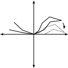
Consider two points in the realization, and a rotation angle with . We seek to apply Lemma 3.1 and so we would like to know that the distance between is increased by the rotation, which means it suffices to show that their squared distance is increased. If both are unmoved by the rotation, or if both are rotated, then the distance between them is unchanged. Thus, we can suppose that is moved, and is fixed. We will consider cylindrical coordinates, with the axis of rotation the center of the cylinder. This causes the height and radius of both points to be unchanged. Further, since we are rotating about an axis which includes two vertexes which are absolute minimums, we can presume that the radii are both non-negative, that the fixed point, , has angle between and , and that the point being rotated, , has angle which starts between and . Let be the difference between and . The height coordinates are both constant, so the difference in the squared distance reduces to the following.
| (3.11) |
Because , we know that initially. Since we can observe that is reduced. This means that is decreased by the move, so the distance between the points is increased. This means that every rotation by an angle with does not decrease thickness, so the particular rotation by has a neighborhood which does not decrease thickness. ∎
Theorem 3.16.
Any knot may be made convex and planar using a sequence of finitely many moves consisting of affine transformations, reflections, or pairs of reflections, such that each move is contained in the closure of the interior of moves which will not increase the thickness.
Proof.
We do this using induction on the number of vertexes which fail to attain the minimum height. If there are no vertexes which fail to attain the minimum height then all vertexes are in a common plane. Applying Theorem 3.12 gives a finite sequence of moves which makes it convex, does not change the height, and is in the closure of the interior of moves which do not decrease the thickness and so we are done. Now suppose that we can achieve the desired result if there are less than vertexes which attain the minimum height, and that is a knot which has exactly vertexes which fail to attain the minimum height. We can then apply Theorem 3.12 to get a finite sequence of reflections which do not affect the height, are in the closure of the interior of moves which do not decrease the thickness, and give us a knot configuration which is convex in projection. Since the height is unchanged we still have vertexes which fail to attain the minimum height. We can then use Theorem 3.15 to get a pair of reflections or a rotation in the closure of the interior of moves which do not decrease thickness, which will give us a knot with fewer than minimum vertexes. Finally, we can use the inductive hypothesis to get a sequence of moves in the closure of the interior of moves which do not decrease thickness which results in a convex planar polygon. Thus, can be made convex and planar using moves in the closure of the interior of moves which do not decrease thickness. Therefore, by induction, any knot can be made convex and planar using a finite sequence of moves in the closure of the interior of moves which do not decrease thickness. ∎
3.3 Convex and Planar made Regular
3.3.1 The Move
The move will be a sequence of six reflections, but the net result can be explained much more clearly, and visualized in figure 15. We will take four vertexes and look at the planar knot as being the quadrilateral joined directly by those four vertexes, along with up to four flaps.
The result of the move is equivalent to allowing only the distinguished four vertexes to pivot in the plane, and then pushing two opposite vertexes together, allowing the complementary two to spread apart. This causes two interior angles to shrink and two interior angles to grow. We will pick two vertexes whose interior angles are large and two whose interior angles are small so applying this move minimally will make one of the four regular.

Informally, the way we achieve this type of move using reflections is that we reflect through a plane containing two of the flexible vertexes to bring the complementary vertexes closer together, and then use a reflection through the pair we moved to make the four planar. Finally we use up to four more reflections to bring the four flaps back into the common plane.
3.3.2 Picking Vertexes
As mentioned above, we find a collection of four vertexes, two which have large interior angle and two which have small interior angle, in an alternating pattern around the knot.
Lemma 3.17.
For any convex non-regular polygon in the plane, there exists an ordered set of four vertexes, with the interior angle of smaller than regular, and the interior angle of larger than regular.
Proof.
For this, we first note that if the polygon is not regular, then it must have a vertex, , with an interior angle which is too big and a vertex, , whose interior angle is too small, since the sum of the angles is fixed. Without loss of generality, choose and to be separated only by vertexes with regular angles in at least one of the arcs. Next, we consider the arc consisting of just the two edges connected to . This arc has longer end to end distance than if the polygon was regular. This means that the complementary arc must also have longer end to end distance. Since we are dealing with a convex polygon, the end to end distance is an increasing function of the interior angles, and so there must be some second vertex which has an interior angle which is too large. This vertex cannot be between and so without loss of generality, choose it to be the closest such vertex to on the other side from . Thus, the arc connecting to through consists only of vertexes with angles which are regular or smaller than regular. This means that this arc has shorter end-to-end distance than in the regular polygon, so the complementary arc has shorter end-to-end distance than the regular polygon, meaning it must also have a vertex, , which has an angle which is smaller than regular. Thus, we have a sequence of ordered vertexes , with having angles which are smaller than regular and with having angles which are bigger than regular. ∎
3.3.3 Choosing Reflections
We will assume the knot lies in the plane and form a transformation of the knot , consisting of up to six reflections which result in begin planar and having more regular vertexes than . The first reflection will reflect the arc connecting to through across a plane which makes an angle of to the plane. There are generally two such choices so we will choose the one which puts the vertex to a non-negative coordinate. The second will reflect the arc connecting to through , and will be chosen in such a way as to make the four vertexes coplanar. There are generally two such choices so choose the one which maximizes the coordinate of . Finally, the four arcs connecting the vertexes of our highlighted quadrilateral may be out of alignment, so we will reflect them each across a plane which will bring them into the common plane of . Again there are two such choices so we will choose the one which moves each flap the shortest distance. This gives a family of transformations, , for each real number, between and , with continuous in . This leads us to the next result.
Theorem 3.18.
Any convex planar knot can be made regular using a sequence of finitely many moves, each move consisting of at most six reflections, with each such move in the interior of moves which do not decrease thickness.
Proof.
We will show that there is a choice of for which has exactly one of the four vertexes have a regular interior angle without switching any of the other four between larger than regular interior angle and smaller than regular interior angle. For this, we consider the vectors , , , and . These are the four edges of the inscribed quadrilateral formed by those four vertexes. We then look at the function . For , . For , . Thus, since is a continuous function and is a continuous function of , we use the intermediate value theorem to observe that there is a choice for which , so and are perpendicular vectors.. The configuration is always planar, so the vectors and are parallel. This means that the two vectors are both parallel and perpendicular, which can only be the case if one of them is the zero vector. Thus, either is zero or is zero, so in , one of the is collinear with and .
For the remainder of the proof . This means that in particular is still an embedding. Thus, we have a well defined notion of the sign of a turning angle, where the sign of all turning angles in are positive. The fact that the interior angle of in is smaller than regular tells us the turning angle at in is larger than regular. Because is collinear with and in , the turning angle of in is negative. This means that by the intermediate value theorem, there exists an angle with the turning angle of in regular.
There may be multiple choices of with having a greater number of regular angles than . We then choose the smallest which makes at least one of the four changing angles regular. Thus, one particular angle is made regular, and the remainder stay on the same side of regular, either staying larger than regular or staying smaller than regular. We note that from corollary 2.4, the long range thickness need not be considered. One possibility is that the smallest angle is unchanged, which means that for any in a neighborhood of , the thickness of is the same as the thickness of . The other possibility is that the smallest angle is one of the and so is larger, meaning that is thicker than and so since thickness is continuous, a neighborhood of does not decrease thickness. Therefore we have increased the number of regular vertexes using a move on the interior of moves which do not decrease thickness. Applying this up to times, where is the number of vertexes, we can guarantee that the end result has at least regular vertexes, and so is the regular planar polygon. ∎
3.4 Result
Theorem 3.19.
Any equilateral polygonal knot can be made into a regular convex planar polygon using a finite number moves, consisting only of rigid motions, or up to six reflections, with each move in the closure of the interior of moves which do not decrease thickness.
Proof.
This is a simple combination of the above theorems. First, Theorem 3.16 shows that a finite number of such moves can make any equilateral polygonal knot planar and convex, and then Theorem 3.18 allows another finite number of such moves to make any equilateral polygonal planar and convex knot regular. This gives us the desired result. ∎
4 Monte-Carlo Markov Chains
In this section, we will prove that we can build an ergodic Markov chain for sampling the space of equilateral knots with thickness. The above theorem will be necessary in showing ergodicity.
4.1 The Markov Chain
The general definition of a Markov chain is a sequence in a state space where each entry in the sequence of states is independent of every state before the immediate predecessor. We will refer to our Markov chain as . Our Markov chain is given by a set of states in , a noise parameter which is an open subset of with a probability measure , and a function . The space of states will be . The noise parameter will be a product of reflection moves. The space of reflection moves is of the form , where is a real number in used to determine if we check the thickness, are a random pair of vertexes, and is an angle. While this isn’t clearly an open subset of , it can be modeled in that way by choosing the continuous variables from a rectangle, and selecting the discreet variables by using a disjoint collection of rectangles. Thus, we use
| (4.1) |
where is the number of edges. This space is a disjoint collection of rectangles. The coordinate is an angle. The width of each rectangle is . Which rectangle a point is in determines the which represents a pair of distinct vertexes. The complete noise space is , where is a cap on how many reflections we are allowed between checking the thickness. We require that so that we may use Theorem 3.19. The probability measure on is just a multiple of the Lebesgue measure on this bounded space, which means that it has a constant probability distribution which is supported on all of and is lower semi-continuous since is open.
The function F in our Markov chain will be defined as follows. We have a collection of probabilities which represent the probability of applying the reflection if we already applied the reflection. Given a we find a sequence of variables , where is the coordinate of . These live in . We find which is one less than the first with , or if no such exists. This is how many reflections we will apply. When we apply a reflection to a knot , we reflect the arc connecting the vertexes and across a plane determined by the angle , where are indicated by which component of we are in and from . Thus, we get a reflection move for each . This lets us define if and otherwise. This means is a piecewise function with two pieces, one is the identity and the other is smooth.
4.2 Forward Accessible
We will use to denote the set of states for which there is a sequence of exactly moves on the interior of a smooth section starting at and ending at . We will also define . One useful property a Markov chain can have is forward accessibility. A Markov chain is forward accessible if is a set with non-empty interior, for every value of . When the motion of the Markov chain is smooth, then the set reduces to simply points reachable in steps, but since our function is merely piecewise smooth we need the more general definition. We will prove our Markov chain is forward accessible. This will be a direct continuation of the conclusion of the previous chapter.
Lemma 4.1.
For every knot , there is a finite sequence of moves , giving a finite sequence of knots , such that , is the regular planar polygon, and each has a neighborhood of moves , with for every .
Proof.
By Theorem 3.19, there is a sequence of moves with , the regular planar polygon, and each move in the closure of the interior of moves which do not decrease thickness. This means that for any open neighborhood of the regular planar polygon, such as int(), we can take a nearby sequence of moves with , in the open set int(), and each on the interior of moves which do not decrease thickness, and so in particular has a neighborhood of moves with for every . We also can use the same theorem to generate a sequence of moves with , the regular planar polygon and each move not decreasing thickness. Since each is on the interior of , there is a neighborhood of each with for every . Concatenating these two sequences of moves, we get the desired result. ∎
Theorem 4.2.
The Markov chain is forward accessible with int for every knot in .
Proof.
In short we will use lemma 4.1 to form a sequence connecting two knots by way of the regular planar polygon.
Let and int(). Then where . By Lemma 4.1, there is a sequence of moves with , the regular planar polygon, and each in an open neighborhood with for all . By the same lemma there is also a sequence of moves with , the regular planar polygon, and each in int(). Each reflection move can be repeated on the image knot, which means that each move has an inverse move . Thus, is the regular planar polygon, , and each is in int(). Since each has an image in the interior of , there is a neighborhood of each, with in for every . Concatenating these two sequences of moves gives a sequence of moves with , , and each move having a neighborhood of moves with for all . This tells us that the sequence of moves is on the interior of a smooth section, and so its image is in . ∎
4.3 T-Chains
A very useful property for a Markov chain to have is being a -chain. The precise definition requires a couple of preliminaries, but we will define it precisely in this section. To motivate it, a -chain has moves of the Markov chain respecting the topology of the state space. We first define the transition probabilities which is the probability of starting at , and ending in after steps. These are examples of transition kernels which are functions with the Borel sets. A transition kernel is stochastic if for all and is substochastic if for all . This allows us to note that is the probability of staying in the total state space after steps, and so these standard probability transition functions are stochastic. From the standard transition probability and a sampling on the natural numbers , we can build the stochastic transition kernel .
This finally allows us to define a -chain as a Markov chain for which there is a substochastic transition kernel and a sampling distribution with , lower semicontinuous, and for every . The lower semicontinuity is what lets us refer to as the continuous piece of , while for every tells us that there is a significant continuous piece of . With these we utilize Propositions 7.1.5 and 6.2.4 from Meyn and Tweedie’s book[9].
Theorem 4.3.
If a Markov chain which is forward accessible has a noise space with a lower semi continuous probability density function , then for each in the state space , there is a sampling distribution and a transition kernel with , and lower semi-continuous for every .
This theorem amounts to taking a neighborhood of the smooth path that starts at and ends in an open set, and using the implicit function theorem to pull that information back into a neighborhood of .
Theorem 4.4.
Suppose a Markov chain whose state space is a subset of and has for every , there is a transition kernel and sampling distribution with , and lower semi-continuous for every . Then the Markov chain is a -chain
Proof.
For each there is a transition kernel given by the hypothesis of the theorem. These kernels have sets which are open since is lower semi-continuous. By assumption, so forms an open cover. By Lindelöf’s theorem, this open cover has a countable subcover . This countable subcover corresponds to a countable set of states with corresponding transition kernels and sampling distributions . Let and . This tells us the following.
| (4.2) | ||||
| (4.3) | ||||
| (4.4) | ||||
| (4.5) | ||||
| (4.6) |
Further, for every since the form an open cover and is lower semi-continuous since each is lower semi-continuous and the series converges uniformly. ∎
We can combine these two results to get the following.
Corollary 4.5.
The Markov chain is a -chain.
Proof.
A sequence of probability distributions is tight if for every , there is a compact set with .
Lemma 4.6.
Any sequence of probability distributions on a compact space is tight.
Proof.
Let be a sequence of probability distributions on a compact space . Since they are probability distributions, which means that for every . ∎
A Markov chain is bounded in probability on average if the sequence is tight.
Corollary 4.7.
The Markov Chain has a compact state space, and so is bounded in probability on average.
4.4 Positive Harris Recurrent
We can talk about the number of times a Markov chain lies in a particular set of states as . This allows us to define Harris recurrent. A Markov chain is Harris recurrent if every set with positive Borel measure has . A Markov chain is positive if there is a probability measure on the state space which is invariant under iteration by the Markov process. Both of these properties are extremely useful, and a Markov chain which satisfies both is called positive Harris recurrent.
A state is reachable if for every open set containing . We note that the regular polygon is reachable using Theorem 3.19. We again can utilize the book by Meyn and Tweedie by quoting proposition 18.3.2[9].
Theorem 4.8.
Suppose that is a -chain with a reachable state. Then is positive Harris if and only if it is bounded in probability on average.
This tells us that our Markov chain is positive Harris recurrent.
4.5 Ergodic
We seek to finish by using the main theorem from Meyn and Tweedies book[9].
Theorem 4.9 (Aperiodic Ergodic Theorem).
Suppose that is an aperiodic Harris recurrent chain, with invariant measure . Then being positive Harris recurrent is equivalent to the following.
For every initial condition ,
| (4.7) |
as , and moreover for any two regular initial distributions ,
| (4.8) |
We have already shown that is a positive Harris recurrent T-chain, so the aperiodic ergodic theorem shows that if the chain is aperiodic then it is ergodic. A chain is aperiodic if there is no period greater than one. A chain is periodic with period if there is a collection of disjoint closed sets with the probability of going from to in exactly one step is one.
Theorem 4.10.
The Markov chain is aperiodic and therefore ergodic
Proof.
Note that if the pair of points through which a potential reflection will take place is chosen to be distance exactly two from each other, then there is a choice of plane which contains the length two arc connecting them. This means that there is a choice of noise parameter which leaves the equilateral knot fixed. Thus, for any set , there is a move which takes a state in to itself. Suppose and are disjoint non-empty closed sets. Then for each in there is a move which fixes and so takes to . This complement is an open set and is a continuous function of so there is a positive probability of going from to . This ensures that no collection of multiple disjoint sets can satisfy the periodicity condition. This shows aperiodicity which then allows us to apply the aperiodic ergodicity theorem to conclude that the Markov chain is ergodic. ∎
5 Conclusion and Future Work
The reflection algorithm with the use of intermediate checks that we have presented here provides a greatly expanded means of analyzing knots with a thickness. This algorithm is significantly faster for sufficiently large thicknesses. Further, the proof that this method is ergodic for every positive thickness ensures that it can be used to analyze every possible feature of geometric knots. This new algorithm provides the means for the careful study of the effects of excluded volume across the entire range of lengths and thicknesses. I hope to have this algorithm used to study the impact of thickness, and to analyze the resulting probability distribution in the space of thick knots.
References
- [1] Sotero Alvarado, Jorge Alberto Calvo, and Kenneth C. Millett. The generation of random equilateral polygons. Journal of Statistical Physicis, 143:102–138, 2011.
- [2] Jason Cantarella and Clayton Shonkwiler. The symplectic geometry of closed equilateral random walks in 3-space.
- [3] James J. Champoux. Dna topoisomerases: structure, function and mechanism. Annual Review of Biochemistry, 70:369–413, 2001.
- [4] S.S Chern. Studies in Global Geometry and Analysis. Prentice-Hall, 1970.
- [5] W. Fiers and R. L. Sinsheimer. The structure of the dna of bacteriophage phi x174. iii. ultracentrifugal evidence for a ring structure. Journa of Molecular Biology, 5:424–434, 1962.
- [6] Branko Grünbaum and Joseph Zaks. Convexification of polygons by flips and by flipturns. Discrete Mathematics, 241(1–3):333 – 342, 2001.
- [7] L. F. Liu, R. E. Depew, and J. C. Wang. Knotted single strand dna formed by treatment with escherichia coli w protein. Journal of Molecular Biology, 106(2):439–452, 1976.
- [8] T. McLeish. A tangled tale of topological fluids. Physics Today, 61(8):40–45, 2008.
- [9] S.P. Meyn and R.L. Tweedie. Markov Chains and Stochastic Stability. Springer-Verlag, 1993.
- [10] Ken Millett. Knotting of regular polygons in 3-space. Journal of Knot Theory and its Ramifications, 3(3):263–278, 1994.
- [11] Kenneth C. Millett, Michael Piatek, and Eric Rawdon. Polygonal knot space near ropelength-minimized knots. Journal of Knot Theory and Its Ramifications, 17(05):601–631, 2008.
- [12] Richard Randell. Conformation spaces of molecular rings. Physical and Theoretical Chemistry, 54:125–140, 1988.
- [13] Eric J. Rawdon. Approximating smooth thickness. Journal of Knot Theory and Its Ramifications, 09(01):113–145, 2000.
- [14] Godfried Toussaint. The Erdős Nagy theorem and its ramifications. Computational Geometry, 31(3):219 – 236, 2005.
- [15] S.A. Waserman, J.M. Dungan, and N.R. Cozzerelli. Discovery of a predicted dna knot substantiates a model for site-specific recombination. Science, 229(4709):171, 1985.