Genetic Algorithm for Chromaticity Correction in Diffraction Limited Storage Rings

The ranking of individuals in a single objective optimization problem is straightforward: the individual with the better objective value is preferred. Ranking in multi-objective optimization problem is more complicated. The core concept is the dominance relationship, which is a way of comparing any two individuals, say $\mathbf{x}^{\left(i\right)}$and $\mathbf{x}^{\left(j\right)}$. They are compared by asking the question: “Does $\mathbf{x}^{\left(i\right)}$dominate $\mathbf{x}^{\left(j\right)}$?” The dominance relationship is defined as [17]:

A sorting algorithm applies the dominance relationship to sort the population from best to worst. There exist many different sorting algorithms. Two algorithms that we have used are NSGA2 and SPEA2. We obtain similar results with both algorithms, but find that the populations resulting from SPEA2 span the objective space more evenly.

For details on SPEA2 see Ref. [14]. In short summary, dominance is determined for every ordered pair of individuals in the population. Each individual in the population is assigned a strength which is the number of individuals it dominates. Then, each individual is assigned a fitness which is the sum of the strengths of all the individuals that dominate it. A lower fitness is better. A ‘clumping’ penalty is added to this fitness based on the shortest distance (in objective space) of the individual to another individual. This encourages the population to span a wider region of the objective space. Incidentally, the clumping penalty makes it unlikely for any two individuals to have the exact same fitness, even if they are both not dominated by any other individual.

Individuals are ordered according to their fitness value. The lowest ranked individuals are deleted from the population. This is typically the worst half or three-quarters of the population each generation. The population is replenished by mating the surviving individuals.

Mating pairs are determined by drawing integers in a procedure called a tournament. Two or more random integers are drawn between $1$ and $N$, where $N$ is the number of surviving individuals. $1$ corresponds to the most fit, and $N$ to the least fit. The individual corresponding to the smallest of the drawn integers is chosen for mating. Thus, individuals with better fitness are more likely to reproduce. Its mate is chosen through the same process. This is repeated until enough pairs have been selected to replenish the population. Each pair generates two offspring.

A two-step process generates two new children from each mating pair. The first step is simulated binary cross-over [18]. Say the two parents are ${\mathbf{x}^{\left(p1\right)}=\left\{x^{\left(p1\right)}_{1},x^{\left(p1\right)}_{2},...,x^{\left(p1\right)}_{n}\right\}}$ and ${\mathbf{x}^{\left(p2\right)}=\left\{x^{\left(p2\right)}_{1},x^{\left(p2\right)}_{2},...,x^{\left(p2\right)}_{n}\right\}}$. They will produce two offspring, $\mathbf{x}^{\left(c1\right)}$ and $\mathbf{x}^{\left(c2\right)}$.

Start with variable $x_{1}^{\left(\cdot\right)}$ and draw a random real $t$ between $0$ and $1$. Compare $t$ to $P_{c}$, which is a parameter between $0$ and $1$ that determines how likely it is that a variable is simply copied from parent to child, as opposed to applying a stochastic function. If $t>P_{c}$, then variable $x^{\left(p1\right)}_{1}$ is simply copied to the child $x^{\left(c1\right)}_{1}$, and $x^{\left(p2\right)}_{1}$ copied to $x^{\left(c2\right)}_{1}$. If $t\leq P_{c}$, then draw another random real $q$ between $0$ and $1$. Then,

and

where $\kappa$ is a parameter that controls the width of the distribution. As depicted in Fig. 1, smaller values of $\kappa$ cause the offspring to explore a broader parameter space. A typical value for $P_{c}$ is $0.8$. This process is repeated for all $n$ variables.

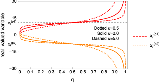
Next a mutator is applied separately to $\mathbf{x}^{\left(c1\right)}$ and $\mathbf{x}^{\left(c2\right)}$. For each variable $i$ in $\mathbf{x}^{\left(c1\right)}$, draw a random real $t$ between $0$ and $1$. Compare $t$ to $P_{m}$, a parameter that determines how likely it is for a variable to undergo mutation. If $t>P_{m}$, the variable is not mutated. If $t\leq P_{m}$, then draw a second random real $m$. Variable $x_{i}^{\left(c1\right)}$ is adjusted according to

and

A typical value for $P_{m}$ is $n^{-1}$, so that on average one variable is mutated per child. $\sigma_{\text{mut}}$ is typically set to about $10\%$ of the reasonable variable strength. $\beta_{m}$ is depicted in Fig. 2.

After $\mathbf{x}^{\left(c1\right)}$, the mutation process is repeated on each variable in $\mathbf{x}^{\left(c2\right)}$ and both are added to the population. New individuals are generated until the population is fully replenished.

Once the population is fully replenished, the worker processes calculate the objectives and constraints of the newly generated individuals. The population, consisting of both the parents and children, is resorted and the least fit are deleted. Some of the children will be more fit and displace the older individuals in the surviving population. So is the overall fitness of the population improved. This process of evaluation, sorting, deletion, and replenishment is looped continually. Each loop is referred to as a generation.

As implemented, there is not actually a clear line between one generation and the next. The algorithm is modified to improve computational efficiency. By far, the most time-consuming step is when the objectives and constraints of an individual are calculated. It could often be the case that many nodes in the cluster sit idle while the last few individuals of a given generation are being evaluated. To avoid this situation, the optimizer initially generates extra individuals equal to the number of cores in the cluster. For example, if the population is set to $300$ and there are $64$ nodes in the cluster, the optimizer will initially generate $364$ individuals. Whenever a core finishes evaluating an individual, the individual is added to the population and the core is always immediately given a new unevaluated individual to process. Whenever the population reaches $300$, it is resorted, culled, and new individuals are bred. These new individuals replenish the pool of individuals awaiting evaluation. This modification to the algorithm improves cluster efficiency. The loss of a clear demarcation between the generations does not seem to negatively impact the evolution of the population.

Dominance constraints are a powerful type of constraint that is unique to multi-objective optimization. It is implemented by modifying the dominance relationship. We apply the dominance relationship as implemented in aPISA [6].

In addition to calculating objective values $\mathbf{f}\left(\mathbf{x}^{\left(i\right)}\right)$ for each individual $i$, we also calculate a vector of constraint values $\mathbf{c}\left(\mathbf{x}^{\left(i\right)}\right)$. For example, say $c_{1}$ is a dominance constraint for the off-momentum horizontal closed orbit $x_{\text{inj}}$ at the injection point, and we wish to constrain $\left|x_{\text{inj}}\right|$ to be less than $x_{\text{max}}$. Then, $c_{1}=x_{\text{max}}-\left|x_{\text{inj}}\right|$. If $c_{1}$ is negative, it indicates that the constraint is violated. The magnitude of $c_{1}$ represents the degree to which it is violated.

Dominance constraints are implemented by replacing the ordinary definition for dominance in Def. 1 with Def. 2. An individual is called infeasible if it violates any of its dominance constraints, else it is called feasible.

The behavior of a genetic algorithm implementing dominance constraints flows through three phases:

1. 1.

   Random population, possibly containing no feasible individuals, spans variable space, sorted according to severity of constraint violations.

2. 2.

   Entire population is feasible and spans feasible region of variable space, sorted according to objective values.

3. 3.

   Population spans variable space that approaches the Pareto optimal objective space.

Notice that if an individual violates any of its dominance constraints, then its objective values are not taken into account during ranking. Therefore, to save computing time, objective values are calculated only for individuals which do not violate any dominance constraints. Dominance constraints are based on variable bounds, closed orbit amplitudes, and chromatic tune shifts. These quantities are orders of magnitude quicker to evaluate than objective values, which are based on particle tracking.

The dynamic apertures are calculated relative to the linear aperture. The linear aperture is the smallest aperture found by projecting the beam chamber from each point in the lattice to the injection point using the linearization of the map about the particle momentum. The linear aperture, in general, depends on the particle momentum. The on-energy linear aperture does not depend on the sextupole and multipole strengths, but the off-energy linear aperture does. The objective function is formulated relative to the linear aperture such that $1.0$ is perfectly bad and $0.0$ is perfectly good,

where $N_{\text{angle}}$ is the number of rays along which the aperture is calculated. $L_{\text{l}}$ is the length of the linear aperture ray. $L_{\text{da}}$ is the length of the dynamic aperture ray. $L_{\text{l}}$ and $L_{\text{da}}$ are depicted in Fig. 3.

The conditional in Eq. 7 reflects our design philosophy that a machine with optimized nonlinearities should behave as if it were linear. The objective function is not rewarded when the dynamic aperture exceeds the linear aperture.

Three objectives are used in our multi-objective optimization problem:

where $\Delta E_{\textrm{+DA}}$ and $\Delta E_{\textrm{-DA}}$ specify the energy offset where dynamic aperture is evaluated. Typical energy offsets are $2\%$ or $3\%$.

Three constraint techniques are used: dominance constraints, modified objective functions, and variable space projection.

Five constraints are implemented as dominance constraints. They are

1. 1.

   $c_{\textrm{mag}}$: Boundary on sextupole and multipole strength.

2. 2.

   $c_{+co}$: Global bound on nonlinear dispersion at $\Delta E_{\textrm{+DA}}$.

3. 3.

   $c_{-co}$: Global bound on nonlinear dispersion at $\Delta E_{\textrm{-DA}}$.

4. 4.

   $c_{+\chi}$: Confine chromatic tune footprint between $0$ and $\Delta E_{+\chi}$.

5. 5.

   $c_{-\chi}$: Confine chromatic tune footprint between $0$ and $\Delta E_{-\chi}$.

The constraint on sextupole and multipole strength is calculated as,

where $K_{i}$ is the strength of magnet $i$, and $x_{i}^{\left(U\right)}$ and $x_{i}^{\left(L\right)}$ are the upper and lower bounds on the magnet strength.

The two constraints on global nonlinear dispersion are calculated as,

where $x^{\left(\textrm{co}\right)}$ is the maximum allowed closed orbit, usually set to millimeter or so. $x_{\textrm{co},i}$ and $\eta_{i}$ are the closed orbit and ordinary dispersion at element $i$.

The positive chromatic footprint between $0$ and $\Delta E_{+\chi}$ is constrained to cross neither the half-integer nor the integer resonances. It is calculated by dividing the interval from $\Delta E=0$ to $\Delta E=\Delta E_{+\chi}$ into $N_{\chi}$ equal segments. The horizontal and vertical tunes are calculated by linearizing the optics about each $\Delta E_{j}\in\left\{\Delta E_{1},\Delta E_{2},...,\Delta E_{+\chi}\right\}$. The smallest of these energy offsets that results in an unstable transfer matrix, or a horizontal or vertical tune that crosses an integer or half-integer resonance, is used to calculate the value of the dominance constraint. The value is calculated as,

If all $\Delta E_{+j}$ are stable and do not cross the half-integer or integer, $c_{+\chi}$ is set to $0$. A similar procedure is used to constrain the negative chromatic tune footprint $c_{-\chi}$.

Two constraints are implemented by modifying the objective functions. The first is a constraint on the minimum size of the off-energy linear aperture and it modifies the off-energy objective functions $f_{+}$ and $f_{-}$. The constraint prevents a failure condition where the optimizer improves the off-energy objectives by making the linear aperture tiny, rather than by growing the dynamic aperture. Setting this constraint to $2$ or $3$ mm is usually sufficient to avoid the condition. If the shortest linear aperture ray at $\Delta E_{\textrm{+DA}}$ or $\Delta E_{\textrm{-DA}}$ is shorter than this constraint, then $f_{+}$ or $f_{-}$ is set to a perfectly bad value of $1$.

The second constraint implemented by modifying the objective functions modifies the on-energy objective function $f_{0}$. It confines the on-energy amplitude dependent tune shift (ADTS). Along the two DA rays closest to the horizontal axis, the horizontal and vertical tunes are calculated. Along the vertical ray, the vertical tune is calculated. This is because the horizontal motion for large vertical and small horizontal offsets is dominated by coupling, rather than by the horizontal optics. The tunes are calculated by summing the element-by-element phase advance in normal mode coordinates. If the tunes of the particle cross the half-integer or integer resonances, then the tracking code considers the particle lost. The apertures along the two horizontal rays and one vertical ray define a ‘clipping’ box. When $f_{0}$ is calculated, all DA rays are clipped at the box.

The chromaticity correction is applied by projecting the $N_{\text{cs}}$-dimensional space of chromatic sextupole strengths onto the $\left(N_{\text{cs}}-2\right)$-dimensional surface on which the horizontal and vertical chromaticities have the desired values. This is possible because chromaticity depends linearly on the sextupole strength. $N_{\text{cs}}$ is the number of chromatic sextupole families in the lattice. A chromaticity response matrix $\mathbf{A}$ is determined numerically,

The Moore-Penrose pseudoinverse $\mathbf{A}_{p}$ of $\mathbf{A}$ is calculated via singular value decomposition (SVD) [19]. Then the thin-QR decomposition [19] $\mathbf{Q}_{1}$ of $\mathbf{I}-\mathbf{A}_{p}\mathbf{A}$ is taken, where $\mathbf{I}$ is the $N_{cs}\times N_{cs}$ identity matrix. Note that $\mathbf{Q}_{1}\in\mathbb{R}^{N_{cs}\times N_{cs}-2}$.

With $\mathbf{A}_{p}$ and $\mathbf{Q}_{1}$ in hand, take any vector $\vec{\omega}\in\mathbb{R}^{Ncs-2}$. The chromatic sextupole strengths $\vec{K}$ given by

result in chromaticities of $\chi_{x0}$ and $\chi_{y0}$.

The algorithm does not operate directly on the chromatic sextupole strengths. Instead it operates on $\vec{\omega}$, thus constraining the chromaticities to the desired values and reducing the dimension of the variable space by $2$.

CANDLE is a proposed $3$ GeV, $216$ m Armenian light source project [21] providing $8.54$ nm horizontal beam emittance. According to the recent developments in storage ring lattice design and magnet technologies a new upgrade prototype has been designed [12], which is constructed of sixteen 4BA cells and provides $1.1$ nm horizontal beam emittance. The study shown here is on this new $1.1$ nm prototype. Each cell is composed of combined function bends with both quadrupole and sextupole moments. Some properties are shown in Tab. 1. Two features which contribute to CANDLE’s nonlinearities are: 1) The sextupole moments are spread out across a broad phase advance. 2) All sextupole moments are in dispersive regions.

The dynamic aperture on-energy and at $\pm 2\%$ are shown in Fig. 8. The horizontal ADTS and chromatic footprint out to $\pm 3\%$ are shown in Fig. 9.

Touschek lifetime results and assumptions are shown in Tab. 3. The momentum aperture calculated from 6D tracking is shown in Fig. 10. The aperture is determined entirely by the RF bucket and not limited by the transverse optics. The phase space portraits are shown in Fig. 11. Optimizing the $\pm 2\%$ dynamic aperture and constraining the chromatic tune footprint to $\pm 3\%$ has successfully optimized the global momentum aperture to at least $\pm 3\%$.