跳到论文正文
W Papers独立论文阅读器 arXiv:1603.02412 论文正文 计算阅读时间 · 0%
引用这篇论文根据当前论文元数据生成,正式投稿前建议核对。


License: arXiv.org perpetual non-exclusive license
arXiv:1603.02412v1 [math.OC] 08 Mar 2016
\typearea

13

Stochastic dual averaging methods using variance reduction techniques for regularized empirical risk minimization problems

Tomoya Murata ††thanks: Email: murata.t.ab@m.titech.ac.jp Affiliation: Department of Mathematical and Computing Sciences, Graduate School of Information Science and Engineering, Tokyo Institute of Technology    Taiji Suzuki ††thanks: Email: suzuki.t.ct@m.titech.ac.jp Affiliation: Department of Mathematical and Computing Sciences, Graduate School of Information Science and Engineering, Tokyo Institute of Technology Affiliation: PRESTO, Japan Science and Technology Agency (JST)
Abstract

We consider a composite convex minimization problem associated with regularized empirical risk minimization, which often arises in machine learning. We propose two new stochastic gradient methods that are based on stochastic dual averaging method with variance reduction. Our methods generate a sparser solution than the existing methods because we do not need to take the average of the history of the solutions. This is favorable in terms of both interpretability and generalization. Moreover, our methods have theoretical support for both a strongly and a non-strongly convex regularizer and achieve the best known convergence rates among existing nonaccelerated stochastic gradient methods.

1 Introduction

We consider the following composite convex minimization problem:

minx∈ℝd{P⁡(x)​=def​F​(x)+R⁡(x)},\underset{x\in\mathbb{R}^{d}}{\mathrm{min}}\ \ \{P(x)\overset{\mathrm{def}}{=}F(x)+R(x)\}, (1)

where F⁡(x)=1n​∑i=1nfi​(x)F(x)=\frac{1}{n}\sum_{i=1}^{n}f_{i}(x). Here each fi:ℝd→ℝf_{i}:\mathbb{R}^{d}\to\mathbb{R} is an LiL_{i}-smooth convex function and R:ℝd→ℝR:\mathbb{R}^{d}\to\mathbb{R} is a relatively simple and (possibly) nondifferentiable convex function. Problems of this form often arise in machine learning and are known as regularized empirical risk minimization.

A traditional method for solving (1) is the (proximal) gradient descent (GD) method. The GD algorithm is very simple and intuitive and achieves a linear convergence rate for a strongly convex regularizer. However, in typical machine learning tasks, the number nn can be very large, and then the iteration cost of GD can be quite expensive.

A popular alternative for solving (1) is the stochastic gradient descent (SGD) method [17, 6, 14]. Since the iteration cost of SGD is very cheap, SGD is suitable to many machine learning tasks. However, SGD only achieves a sublinear convergence rate and is ultimately slower than GD.

Recently, a number of (first-order) stochastic gradient methods using variance reduction techniques, which utilize the finite sum structure of problem (1), have been proposed [11, 12, 7, 21, 10, 4, 1]. The iteration costs of these methods are the same as that of SGD, and, moreover, they achieve a linear convergence rate for a strongly convex objective.

The stochastic average gradient (SAG) method [11, 12] can be used to treat the special case of problem (1) with R=0R=0. To the best of our knowledge, SAG is the first variance reduction algorithm that achieves a linear convergence rate for a strongly convex objective. SAGA [4] is a modified SAG algorithm that not only achieves a linear convergence rate for a strongly convex objective but also can handle a nondifferentiable and non-strongly convex regularizer. However, for a non-strongly convex regularizer, SAGA needs to output the average of the whole history of the solutions for a convergence guarantee whereas SAG and SAGA do not for a strongly convex objective.

In contrast, the stochastic variance reduced gradient (SVRG) method [7, 21] adopts a different variance reduction scheme from SAG and SAGA, and in Acc-SVRG [10] a momentum scheme is applied to SVRG. These methods do not have theoretical support for a non-strongly convex regularizer but they achieve a linear convergence rate for a strongly convex objective. (SVRG needs to output the average of the generated solutions in the last stage for a convergence guarantee whereas Acc-SVRG does not.) UniVR [1] is an extension of SVRG and can handle a non-strongly convex regularizer and achieves an O⁡(n​log​1ε+L¯ε)O\left(n\mathrm{log}\frac{1}{\varepsilon}+\frac{\bar{L}}{\varepsilon}\right) rate (where the OO notation means the order of the necessary number of the gradient evaluations), which is faster than the O⁡(n+Lmaxε)O\left(\frac{n+L_{\mathrm{max}}}{\varepsilon}\right) rate of SAGA for 𝔼⁡[P⁡(x)−P⁡(x∗)]≤ε\mathbb{E}[P(x)-P(x_{*})]\leq\varepsilon, L¯=(1/n)​∑i=1nLi\bar{L}=(1/n)\sum_{i=1}^{n}L_{i}, and Lmax=max⁡{L1,…,Ln}L_{\mathrm{max}}={\mathrm{max}}\{L_{1},\ldots,L_{n}\}. However, UniVR also needs to output the average of the generated solutions in the last stage for convergence guarantees for both strongly and non-strongly convex regularizers.

In summary, the algorithms used in these methods often need to output the average of the history of the solutions as a final solution for convergence guarantees (and, especially, for a non-strongly convex regularizer, all of these methods need to take the average). This requirement is unsatisfactory for a sparsity-inducing regularizer because the average of the previous solutions could be nonsparse.

In this paper, we propose two new stochastic gradient methods using variance reduction techniques: the stochastic variance reduced dual averaging (SVRDA) method and the stochastic average dual averaging (SADA) method. Compared to previous stochastic optimization methods, the main advantages of our algorithms are as follows:

  • •

    Nice sparsity recovery performance: Our algorithms do not need to take the average of the history of the solutions whereas the existing ones do. This property often leads to sparser solutions than the existing methods for sparsity-inducing regularizers.

  • •

    Fast convergence: Our algorithms achieve the best known convergence rates among the existing nonaccelerated stochastic gradient methods for both strongly and non-strongly convex regularizers. Experimentally, our algorithms show comparable or superior convergence speed to that of the existing methods.

2 Assumptions and notation

We make the following assumptions for our theory:

Assumption 1.

Each fif_{i} is convex and differentiable, and its gradient is LiL_{i}-Lipschitz continuous, i.e.,

‖∇fi​(x)−∇fi​(y)‖2≤Li​‖x−y‖2(∀x,y∈ℝd).\displaystyle||\nabla f_{i}(x)-\nabla f_{i}(y)||_{2}\leq L_{i}||x-y||_{2}\hskip 14.22636pt(\forall x,y\in\mathbb{R}^{d}). (2)

Condition (2) is equivalent to the following conditions (see [9]):

fi​(y)≤fi​(x)+⟨y−x,∇fi​(x)⟩+Li2​‖x−y‖22(∀x,y∈ℝd)f_{i}(y)\leq f_{i}(x)+\langle y-x,\nabla f_{i}(x)\rangle+\frac{L_{i}}{2}||x-y||_{2}^{2}\hskip 14.22636pt(\forall x,y\in\mathbb{R}^{d})

and

fi​(x)+⟨y−x,∇fi​(x)⟩+12​Li​‖∇fi​(x)−∇fi​(y)‖22≤fi​(y)(∀x,y∈ℝd).f_{i}(x)+\langle y-x,\nabla f_{i}(x)\rangle+\frac{1}{2L_{i}}||\nabla f_{i}(x)-\nabla f_{i}(y)||_{2}^{2}\leq f_{i}(y)\hskip 14.22636pt(\forall x,y\in\mathbb{R}^{d}).
Assumption 2.

The regularization function RR is μ\mu-strongly convex (and it is possible that μ=0\mu=0), i.e.,

R(y)≥R(x)+ξT(y−x)+μ2||y−x||22(∀x,y∈ℝd,∀ξ∈∂R(x)),R(y)\geq R(x)+\xi^{T}(y-x)+\frac{\mu}{2}||y-x||_{2}^{2}\hskip 14.22636pt(\forall x,y\in\mathbb{R}^{d},\forall\xi\in\partial R(x)),

where ∂R⁡(x)\partial R(x) denotes the set of the subgradients of RR at xx.

Observe that, if the regularization function RR is μ\mu-strongly convex, then the objective function PP is also μ\mu-strongly convex. It is well known that a strongly convex function with μ>0\mu>0 has a unique minimizer.

Assumption 3.

The regularization function RR is relatively simple, which means that the proximal mapping of R,R,

proxR​(y)=argminx∈ℝd​{12​‖x−y‖22+R⁡(x)},\mathrm{prox}_{R}(y)=\underset{x\in\mathbb{R}^{d}}{\mathrm{argmin}\ }\left\{\frac{1}{2}||x-y||_{2}^{2}+R(x)\right\},

can be efficiently computed.

Since the function (1/2)​‖x−y‖22+R⁡(x)(1/2)||x-y||_{2}^{2}+R(x) is 1+μ1+\mu-strongly convex, the function proxR\mathrm{prox}_{R} is well defined regardless of the strong convexity of RR. Note that RR is not necessarily differentiable.

Assumption 4.

There exists a minimizer x∗x_{*} of problem (1).

In addition, we define L¯=(1/n)​∑i=1nLi\bar{L}=(1/n)\sum_{i=1}^{n}L_{i}. Moreover, we define the probability distribution QQ on the set {1,2,…,n}\{1,2,\ldots,n\} by Q={qi}i∈{1,2,…,n}={Lin​L¯}i∈{1,2,…,n}Q=\{q_{i}\}_{i\in\{1,2,\ldots,n\}}=\left\{\frac{L_{i}}{n\bar{L}}\right\}_{i\in\{1,2,\ldots,n\}}. This probability distribution is used to randomly pick up a data point in each iteration. By employing nonuniform distribution, we can improve the convergence as in [21].

Many regularized empirical risk minimization problems in machine learning satisfy these assumptions. For example, given a set of training examples (a1,b1),(a2,b2),…,(an,bn)(a_{1},b_{1}),(a_{2},b_{2}),\ldots,(a_{n},b_{n}), where ai∈ℝda_{i}\in\mathbb{R}^{d} and bi∈ℝb_{i}\in\mathbb{R}, if we set fi​(x)=(1/2)​(ai⊤​x−bi)2f_{i}(x)=(1/2)(a_{i}^{\top}x-b_{i})^{2} and R⁡(x)=λ​‖x‖1R(x)=\lambda||x||_{1}, we get Lasso regression. Then the above assumptions are satisfied with Li=‖ai‖2L_{i}=||a_{i}||_{2}, μ=0\mu=0, and proxR​(y)=(sign⁡(yj)​max​{|yj|−λ,0})j=1d\mathrm{prox}_{R}(y)=(\mathrm{sign}(y_{j})\mathrm{max}\{|y_{j}|-\lambda,0\})_{j=1}^{d}. If we set fi​(x)=log⁡(1+exp⁡(−bi​ai⊤​x))f_{i}(x)=\mathrm{log}(1+\mathrm{exp}(-b_{i}a_{i}^{\top}x)) and R⁡(x)=λ1​‖x‖1+(λ2/2)​‖x‖22R(x)=\lambda_{1}||x||_{1}+(\lambda_{2}/2)||x||_{2}^{2}, we get logistic elastic net regression. Then the above assumptions are satisfied with Li=‖ai‖22/4L_{i}=||a_{i}||_{2}^{2}/4, μ=λ2\mu=\lambda_{2}, and proxR​(y)=(1/(1+λ2))​(sign⁡(yj)​max​{|yj|−λ1,0})j=1d\mathrm{prox}_{R}(y)=(1/(1+\lambda_{2}))(\mathrm{sign}(y_{j})\mathrm{max}\{|y_{j}|-\lambda_{1},0\})_{j=1}^{d}.

3 Related work and our contribution

In this section, we comment on the relationships between our methods and several closely related methods.

Standard methods for solving problem (1) are the GD method and the dual averaging (DA) method [8]. These methods take the following update rules:

xt=\displaystyle x_{t}= prox1η​R(xt−1−1η∇F(xt−1)) (GD),\displaystyle\mathrm{prox}_{\frac{1}{\eta}R}\left(x_{t-1}-\frac{1}{\eta}\nabla F(x_{t-1})\right)\text{\hskip 28.45274pt(GD), }
xt=\displaystyle x_{t}= prox1η​t​R​(x0−1η​∑τ=1t∇F​(xτ−1))​ (DA),\displaystyle\mathrm{prox}_{\frac{1}{\eta}tR}\left(x_{0}-\frac{1}{\eta}\sum_{\tau=1}^{t}\nabla F(x_{\tau-1})\right)\text{\hskip 11.38092pt(DA), }

where x0x_{0} is an initial vector and 1/η1/\eta is a constant step size. GD and DA achieve linear convergence rates for a strongly convex regularizer (where, for DA, we need to borrow a multistage scheme as in [2]). However, when the number of data nn is very large, these methods can be quite expensive because they require O⁡(n​d)O(nd) computation for each update.

Effective alternatives are the SGD method [17, 6, 14] and the regularized dual averaging (RDA) method [20]. These methods randomly draw ii in {1,2,…,n}\{1,2,\ldots,n\} and use ∇fi\nabla f_{i} as an estimator of the full gradient ∇F\nabla F in each iteration:

xt=\displaystyle x_{t}= prox1ηt​R(xt−1−1ηt∇fit(xt−1)) (SGD),\displaystyle\mathrm{prox}_{\frac{1}{\eta_{t}}R}\left(x_{t-1}-\frac{1}{\eta_{t}}\nabla f_{i_{t}}(x_{t-1})\right)\text{\hskip 28.45274pt(SGD), }
xt=\displaystyle x_{t}= prox1ηt​t​R​(x0−1ηt​∑τ=1t∇fiτ​(xτ−1))​ (RDA),\displaystyle\mathrm{prox}_{\frac{1}{\eta_{t}}tR}\left(x_{0}-\frac{1}{\eta_{t}}\sum_{\tau=1}^{t}\nabla f_{i_{\tau}}(x_{\tau-1})\right)\text{\hskip 9.10509pt(RDA), }

where 1/ηt1/\eta_{t} is a decreasing step size. These methods only require O⁡(d)O(d) computation for each iteration and are suitable for large-scale problems in machine learning. However, though ∇fi\nabla f_{i} is an unbiased estimator of ∇F\nabla F, it generally has a large variance, which causes slow convergence. As a result, these methods only achieve sublinear convergence rates even when the regularizer is strongly convex. One of simple solutions of this problem is to use a mini-batch strategy [3, 5]. However, a mini-batch strategy still gives sublinear convergence.

In recent years, a number of (first-order) stochastic gradient methods using variance reduction techniques, which utilize the finite sum structure of problem (1), have been proposed [11, 12, 7, 21, 10, 4, 1]. These methods apply a variance reduction technique to SGD. For example, SVRG [7, 21] takes the following update rules:

x~=x~s−1\displaystyle\widetilde{x}=\widetilde{x}_{s-1}
for ​t=1​ to ​m\displaystyle\text{for }t=1\text{ to }m
Draw ​it​ randomly from ​{1,2,…,n}\displaystyle\hskip 14.22636pt\text{Draw }i_{t}\text{ randomly from }\{1,2,\ldots,n\}
vt=∇fit​(xt−1)−∇fit​(x~)+∇F​(x~)\displaystyle\hskip 14.22636ptv_{t}=\nabla f_{i_{t}}(x_{t-1})-\nabla f_{i_{t}}(\widetilde{x})+\nabla F(\widetilde{x})
xt=prox1η​R​(xt−1−1η​vt)\displaystyle\hskip 14.22636ptx_{t}=\mathrm{prox}_{\frac{1}{\eta}R}\left(x_{t-1}-\frac{1}{\eta}v_{t}\right)
x~s=1m​∑t=1mxt.\displaystyle\widetilde{x}_{s}=\frac{1}{m}\sum_{t=1}^{m}x_{t}.

vtv_{t} is an unbiased estimator of ∇F​(xt−1)\nabla F(x_{t-1}) and one can show that its variance is “reduced”:

E​‖vt−∇F​(xt−1)‖2≤4​L¯​[P⁡(xt−1)−P⁡(x∗)+P⁡(x~)−P⁡(x∗)].\mathrm{E}||v_{t}-\nabla F(x_{t-1})||^{2}\leq 4\bar{L}[P(x_{t-1})-P(x_{*})+P(\widetilde{x})-P(x_{*})].

This means that the variance of the estimator vtv_{t} converges to zero as xtx_{t} and x~\widetilde{x} to x∗x_{*}. In this sense, vtv_{t} is a better estimator of ∇F​(xt−1)\nabla F(x_{t-1}) than the simple estimator ∇fit​(xt−1)\nabla f_{i_{t}}(x_{t-1}). Indeed, these methods achieve linear convergence rates for a strongly convex regularizer.

However, these methods often need to take the average of the previous solutions for convergence guarantee. For example, SVRG and UniVR [1] require taking the average of the history of the solutions in the last stage. SAGA [4] also requires taking the average of all previous solutions for a non-strongly convex regularizer, though it does not for a strongly convex regularizer. For a sparsity-inducing regularizer, this requirement is unsatisfactory because taking the average could cause a nonsparse solution even though the optimal solution is sparse.

In contrast, our proposed methods have theoretical convergence guarantees without taking the average of the previous solutions for both strongly and non-strongly convex regularizers. The basic idea of our methods is simple: We apply a variance reduction technique to RDA rather than to SGD. For example, using an analogy to SVRG, we naturally get the following algorithm:

x~=x~s−1\displaystyle\widetilde{x}=\widetilde{x}_{s-1}
for ​t=1​ to ​m\displaystyle\text{for }t=1\text{ to }m
Draw ​it​ randomly from ​{1,2,…,n}\displaystyle\hskip 14.22636pt\text{Draw }i_{t}\text{ randomly from }\{1,2,\ldots,n\}
vt=∇fit​(xt−1)−∇fit​(x~)+∇F​(x~)\displaystyle\hskip 14.22636ptv_{t}=\nabla f_{i_{t}}(x_{t-1})-\nabla f_{i_{t}}(\widetilde{x})+\nabla F(\widetilde{x})
xt=prox1η​t​R​(x0−1η​∑τ=1tvτ)\displaystyle\hskip 14.22636ptx_{t}=\mathrm{prox}_{\frac{1}{\eta}tR}\left(x_{0}-\frac{1}{\eta}\sum_{\tau=1}^{t}v_{\tau}\right)
x~s=1m​∑t=1mxt.\displaystyle\widetilde{x}_{s}=\frac{1}{m}\sum_{t=1}^{m}x_{t}.

However, this algorithm is not sufficient because the final solution has to be the average of the previous solutions for convergence guarantees (a situation that is similar to RDA). Hence we borrow a momentum scheme and an additional SGD step. (For more detail, see Section 4.) Then the algorithm does not need to take the average of the previous solutions for convergence guarantees even when the regularizer is non-strongly convex. We call this algorithm SVRDA. Similarly, we can apply the dual averaging scheme to SAGA and we call this algorithm SADA.

Comparisons of the properties of these methods are summarized in Table 1. “Gradient complexity” indicates the order of the number of the necessary gradient evaluations for 𝔼⁡[P⁡(x)−P⁡(x∗)]≤ε\mathbb{E}[P(x)-P(x_{*})]\leq\varepsilon (or 𝔼​‖x−x∗‖22≤ε\mathbb{E}||x-x_{*}||_{2}^{2}\leq\varepsilon). “Final output” indicates whether the (theoretically guaranteed) final solution is generated from the (weighted) average of previous iterates (Avg) or from the proximal mapping (Prox). For sparsity-inducing regularizers, the solution generated from the proximal mapping is often sparser than the averaged solution. As we can see from Table 1, the proposed SVRDA and SADA both possess good properties in comparison with state-of-the-art stochastic gradient methods.

Strongly convex Non-strongly convex
Gradient complexity Final output Gradient complexity Final output Memory cost
SAG [11, 12] O⁡((n+Lmaxμ)​log​1+Lmax/nε)O\left(\left(n+\frac{L_{\mathrm{max}}}{\mu}\right)\mathrm{log}\frac{1+L_{\mathrm{max}}/n}{\varepsilon}\right) Prox O⁡(n+Lmaxε)O\left(\frac{n+L_{\mathrm{max}}}{\varepsilon}\right) Avg O⁡(n​d)O(nd)
SVRG [7, 21] O⁡((n+L¯μ)​log​1ε)O\left(\left(n+\frac{\bar{L}}{\mu}\right)\mathrm{log}\frac{1}{\varepsilon}\right) Avg No direct analysis O⁡(d)O(d)
Acc-SVRG [10] O⁡((n+min⁡{L¯μ,n​L¯μ})​log​1ε)O\left(\left(n+\mathrm{min}\left\{\frac{\bar{L}}{\mu},n\sqrt{\frac{\bar{L}}{\mu}}\right\}\right)\mathrm{log}\frac{1}{\varepsilon}\right) Prox No direct analysis O⁡(d)O(d)
SAGA [4] O⁡((n+Lmaxμ)​log​1+n/Lmaxε)O\left(\left(n+\frac{L_{\mathrm{max}}}{\mu}\right)\mathrm{log}\frac{1+n/L_{\mathrm{max}}}{\varepsilon}\right) Prox O⁡(n+Lmaxε)O\left(\frac{n+L_{\mathrm{max}}}{\varepsilon}\right) Avg O⁡(n​d)O(nd)
UniVR [1] O⁡((n+L¯μ)​log​1ε)O\left(\left(n+\frac{\bar{L}}{\mu}\right)\mathrm{log}\frac{1}{\varepsilon}\right) Avg O⁡(n​log​1ε+L¯ε)O\left(n\mathrm{log}\frac{1}{\varepsilon}+\frac{\bar{L}}{\varepsilon}\right) Avg O⁡(d)O(d)
SVRDA O⁡((n+L¯μ)​log​1ε)O\left(\left(n+\frac{\bar{L}}{\mu}\right)\mathrm{log}\frac{1}{\varepsilon}\right) Prox O⁡(n​log​1ε+L¯ε)O\left(n\mathrm{log}\frac{1}{\varepsilon}+\frac{\bar{L}}{\varepsilon}\right) Prox O⁡(d)O(d)
SADA O⁡((n+Lmaxμ)​log​1ε)O\left(\left(n+\frac{L_{\mathrm{max}}}{\mu}\right)\mathrm{log}\frac{1}{\varepsilon}\right) Prox O⁡(n​log​1ε+Lmaxε)O\left(n\mathrm{log}\frac{1}{\varepsilon}+\frac{L_{\mathrm{max}}}{\varepsilon}\right) Prox O⁡(n​d)O(nd)
Table 1: Summary of different stochastic gradient methods that use variance reduction techniques

4 Algorithm description

In this section, we illustrate the proposed methods.

4.1 The SVRDA method

We provide details of the SVRDA method in Algorithm 1. The SVRDA method adopts a multistage scheme. Step (4) generates a variance reduced estimator of the full gradient with nonuniform sampling and is the same as SVRG [7, 21]. Update rules (5) and (6) are the dual averaging update and the gradient descent update, respectively. The SVRDA method combines these two update rules. This idea is similar to the ORDA method [2]. As in (3), for a non-strongly convex regularizer, we have to exponentially increase the iteration number in each inner loop whereas we can use a common fixed iteration number in each inner loop for a strongly convex regularizer. Note that the computational cost of each iteration in the inner loop of the SVRDA method is O⁡(d)O(d) rather than O⁡(n​d)O(nd). Also note that SVRDA outputs the solution generated from the proximal mapping rather than the average of previous iterates. For a strongly convex regularizer, SVRDA can output both x~S\widetilde{x}_{S} (the gradient descent step’s output) and v~S\widetilde{v}_{S} (the dual averaging step’s output) as a final solution. This is because the convergence of 𝔼​‖v~s−x∗‖22\mathbb{E}||\widetilde{v}_{s}-x_{*}||_{2}^{2} is guaranteed with a linear convergence rate whereas the theoretical convergence of 𝔼⁡[P⁡(v~s)−P⁡(x∗)]\mathbb{E}[P(\widetilde{v}_{s})-P(x_{*})] is not guaranteed. Outputting v~S\widetilde{v}_{S} experimentally leads to better sparsity recovery performance than outputting x~S\widetilde{x}_{S} (see Section 6).

Algorithm 1 SVRDA
0:  x~0∈ℝd\widetilde{x}_{0}\in\mathbb{R}^{d}, η>0\eta>0, m1∈ℕm_{1}\in\mathbb{N}, S∈ℕS\in\mathbb{N}.
 v~0=x~0\widetilde{v}_{0}=\widetilde{x}_{0}
 α={14(μ>0)0(μ=0)\alpha=\begin{cases}\frac{1}{4}&(\mu>0)\\ 0&(\mu=0)\end{cases}
 for s=1s=1 to SS do
   x0=x~s−1x_{0}=\widetilde{x}_{s-1}, v0=(1−α)​v~s−1+α​x~s−1,u0=v0v_{0}=(1-\alpha)\widetilde{v}_{s-1}+\alpha\widetilde{x}_{s-1},u_{0}=v_{0}, g¯0=0\bar{g}_{0}=0
   
ms={m1(μ>0)2s−1​m1(μ=0)m_{s}=\begin{cases}m_{1}&(\mu>0)\\ 2^{s-1}m_{1}&(\mu=0)\end{cases} (3)
  
   for t=1t=1 to msm_{s} do
     pick it∈{1,2,…,n}i_{t}\in\{1,2,\ldots,n\} randomly according to QQ
     
gt\displaystyle g_{t} =(∇fit​(ut−1)−∇fit​(x0))/n​qit+∇F​(x0)\displaystyle=(\nabla f_{i_{t}}(u_{t-1})-\nabla f_{i_{t}}(x_{0}))/nq_{{i}_{t}}+\nabla F(x_{0})\hskip 56.9055pt (4)
g¯t\displaystyle\bar{g}_{t} =(1−1t)​g¯t−1+1t​gt\displaystyle=\left(1-\frac{1}{t}\right)\bar{g}_{t-1}+\frac{1}{t}g_{t}
vt\displaystyle v_{t} =argminx∈ℝd​{⟨g¯t,x⟩+R⁡(x)+η2​t||x−v0||22}\displaystyle=\underset{x\in\mathbb{R}^{d}}{\mathrm{argmin}\ }\left\{\langle\bar{g}_{t},x\rangle+R(x)+\frac{\eta}{2t}||x-v_{0}||_{2}^{2}\right\}
=prox1η​t​R​(v0−1η​t​g¯t)\displaystyle=\mathrm{prox}_{\frac{1}{\eta}tR}\left(v_{0}-\frac{1}{\eta}t\bar{g}_{t}\right) (5)
xt\displaystyle x_{t} =argminx∈ℝd​{⟨gt,x⟩+R⁡(x)+η​t2||x−ut−1||22}\displaystyle=\underset{x\in\mathbb{R}^{d}}{\mathrm{argmin}\ }\left\{\langle g_{t},x\rangle+R(x)+\frac{\eta t}{2}||x-u_{t-1}||_{2}^{2}\right\}
=prox1η​t​R​(ut−1−1η​t​gt)\displaystyle=\mathrm{prox}_{\frac{1}{\eta t}R}\left(u_{t-1}-\frac{1}{\eta t}g_{t}\right) (6)
ut\displaystyle u_{t} =(1−1t+1)​xt+1t+1​vt\displaystyle=\left(1-\frac{1}{t+1}\right)x_{t}+\frac{1}{t+1}v_{t}
   end for
   x~s=xms\widetilde{x}_{s}=x_{m_{s}}, v~s=vms\widetilde{v}_{s}=v_{m_{s}}
 end for
 x~S\widetilde{x}_{S} or v~S\widetilde{v}_{S} (μ>0\mu>0), x~S\widetilde{x}_{S} (μ=0\mu=0).

4.2 The SADA method

We provide details of the SADA method in Algorithm 2. The algorithm is similar to SVRDA (Algorithm 1). The main difference from the SVRDA method is the update rule (7). This step reduces the variance of the approximation of the full gradient using a SAGA [4] type variance reduction technique rather than SVRG. Note that SADA is a multistage algorithm like SVRG and SVRDA whereas SAGA is a single-stage algorithm. To the best of our knowledge, there exists no single-stage dual averaging algorithm that achieves a linear convergence rate for a strongly convex regularizer. This is probably because of the limitations of the single-stage dual averaging algorithms. Also note that we adopt uniform sampling for SADA. Schmidt et al. [13] have considered a nonuniform sampling scheme for SAGA on the special setting R=0R=0 in (1), but their methods require two gradient evaluations in one iteration and it is not satisfactory. For this reason, we do not adopt nonuniform sampling schemes for SADA in this paper. SADA has theoretically similar properties to SVRDA except for the difference of the sampling scheme, and experimentally SADA sometimes outperforms SVRDA (see Section 6).

Algorithm 2 SADA
0:  x~0∈ℝd\widetilde{x}_{0}\in\mathbb{R}^{d}, η>0\eta>0, m1∈ℕm_{1}\in\mathbb{N}, S∈ℕS\in\mathbb{N}
 v~0=x~0\widetilde{v}_{0}=\widetilde{x}_{0}
 α={14(μ>0)0(μ=0)\alpha=\begin{cases}\frac{1}{4}&(\mu>0)\\ 0&(\mu=0)\end{cases}
 for s=1s=1 to SS do
   x0=x~s−1x_{0}=\widetilde{x}_{s-1}, v0=(1−α)​v~s−1+α​x~s−1v_{0}=(1-\alpha)\widetilde{v}_{s-1}+\alpha\widetilde{x}_{s-1}, u0=v0u_{0}=v_{0}, g¯0=0\bar{g}_{0}=0, ϕi0=x0​(i=1,2,…,n)\phi_{i}^{0}=x_{0}\ (i=1,2,\ldots,n)
   
ms={m1(μ>0)2s−1​m1(μ=0)m_{s}=\begin{cases}m_{1}&(\mu>0)\\ 2^{s-1}m_{1}&(\mu=0)\end{cases}
   for t=1t=1 to msm_{s} do
     pick it∈{1,2,…,n}i_{t}\in\{1,2,\ldots,n\} uniformly at random
     
ϕitt\displaystyle\phi_{i_{t}}^{t} =ut−1,ϕit=ϕit−1​(i≠it)\displaystyle=u_{t-1},\phi_{i}^{t}=\phi_{i}^{t-1}(i\neq i_{t})
gt\displaystyle g_{t} =∇fit​(ϕitt)−∇fit​(ϕitt−1)+1n​∑i=1n∇fi​(ϕit−1)\displaystyle=\nabla f_{i_{t}}(\phi_{i_{t}}^{t})-\nabla f_{i_{t}}(\phi_{i_{t}}^{t-1})+\frac{1}{n}\sum_{i=1}^{n}\nabla f_{i}(\phi_{i}^{t-1})\hskip 56.9055pt (7)
g¯t\displaystyle\bar{g}_{t} =(1−1t)​g¯t−1+1t​gt\displaystyle=\left(1-\frac{1}{t}\right)\bar{g}_{t-1}+\frac{1}{t}g_{t}
vt\displaystyle v_{t} =argminx∈ℝd​{⟨g¯t,x⟩+R⁡(x)+η2​t||x−v0||22}\displaystyle=\underset{x\in\mathbb{R}^{d}}{\mathrm{argmin}\ }\left\{\langle\bar{g}_{t},x\rangle+R(x)+\frac{\eta}{2t}||x-v_{0}||_{2}^{2}\right\}
=proxtη​R​(v0−tη​g¯t)\displaystyle=\mathrm{prox}_{\frac{t}{\eta}R}\left(v_{0}-\frac{t}{\eta}\bar{g}_{t}\right)
xt\displaystyle x_{t} =argminx∈ℝd​{⟨gt,x⟩+R⁡(x)+η​t2||x−ut−1||22}\displaystyle=\underset{x\in\mathbb{R}^{d}}{\mathrm{argmin}\ }\left\{\langle g_{t},x\rangle+R(x)+\frac{\eta t}{2}||x-u_{t-1}||_{2}^{2}\right\}
=prox1η​t​R​(ut−1−1η​t​gt)\displaystyle=\mathrm{prox}_{\frac{1}{\eta t}R}\left(u_{t-1}-\frac{1}{\eta t}g_{t}\right)
ut\displaystyle u_{t} =(1−1t+1)​xt+1t+1​vt\displaystyle=\left(1-\frac{1}{t+1}\right)x_{t}+\frac{1}{t+1}v_{t}
   end for
   x~s=xms\widetilde{x}_{s}=x_{m_{s}}, v~s=vms\widetilde{v}_{s}=v_{m_{s}}
 end for
 x~S\widetilde{x}_{S} or v~S\widetilde{v}_{S} (μ>0\mu>0), x~S\widetilde{x}_{S} (μ=0\mu=0).

5 Convergence analysis

Now we give a convergence analysis of our algorithms. In this section, all norms ||⋅||||\cdot|| mean the L2L_{2}-norm ||⋅||2||\cdot||_{2}.

5.1 Convergence analysis of SVRDA

In this subsection, we give the convergence analysis of SVRDA.

Theorem 5.1.

Suppose that Assumptions 1, 2, 3, and 4 hold (and it is possible that μ=0\mu=0). Let x0∈ℝdx_{0}\in\mathbb{R}^{d}, η=4​L¯\eta=4\bar{L}, m1∈ℕ,m_{1}\in\mathbb{N,} and 0≤α≤10\leq\alpha\leq 1. Then the SVRDA algorithm satisfies

𝔼⁡[P⁡(x~s)−P⁡(x∗)]+η+ms​μ2​ms​𝔼​‖v~s−x∗‖2\displaystyle\mathbb{E}\left[P(\widetilde{x}_{s})-P(x_{*})\right]+\frac{\eta+m_{s}\mu}{2m_{s}}\mathbb{E}||\widetilde{v}_{s}-x_{*}||^{2}
≤\displaystyle\leq 12​𝔼​[P⁡(x~s−1)−P⁡(x∗)]+(α​η2​ms−μ4)​𝔼​‖x~s−1−x∗‖2+(1−α)​η2​ms​𝔼​‖v~s−1−x∗‖2.\displaystyle\frac{1}{2}\mathbb{E}[P(\widetilde{x}_{s-1})-P(x_{*})]+\left(\frac{\alpha\eta}{2m_{s}}-\frac{\mu}{4}\right)\mathbb{E}||\widetilde{x}_{s-1}-x_{*}||^{2}+\frac{(1-\alpha)\eta}{2m_{s}}\mathbb{E}||\widetilde{v}_{s-1}-x_{*}||^{2}.
Remark.

On inequality (8) in Appendix A, we can apply a tighter bound and η\eta can be smaller than 4​L¯4\bar{L} for satisfying Theorem 5.1. This means that we can get a larger step size 1η\frac{1}{\eta} than 14​L¯\frac{1}{4\bar{L}} and have a theoretically tighter bound. However, practically, if we tune η\eta, it makes little difference and thus we omit it in this paper.

The proof of Theorem 5.1 is given in Appendix A. Using this theorem, we derive recursive inequalities relative to 𝔼⁡[P⁡(x~s)−P⁡(x∗)]\mathbb{E}[P(\widetilde{x}_{s})-P(x_{*})] and 𝔼​‖v~s−x∗‖2\mathbb{E}||\widetilde{v}_{s}-x_{*}||^{2}. Based on Theorem 5.1, we obtain the linear convergence of SVRDA for μ>0\mu>0.

Corollary 5.2 (for a strongly convex regularizer).

Suppose that Assumptions 1, 2, 3, and 4 hold. Moreover, assume that μ>0\mu>0. Let x0∈ℝdx_{0}\in\mathbb{R}^{d}, η=4​L¯\eta=4\bar{L}, m1=η2​μm_{1}=\frac{\eta}{2\mu}, S∈ℕ,S\in\mathbb{N,} and α=14\alpha=\frac{1}{4}. Then the SVRDA algorithm satisfies

𝔼⁡[P⁡(x~S)−P⁡(x∗)]+3​μ2​𝔼​‖v~S−x∗‖2≤12S​[P⁡(x~0)−P⁡(x∗)+3​μ2​‖x~0−x∗‖2].\mathbb{E}[P(\widetilde{x}_{S})-P(x_{*})]+\frac{3\mu}{2}\mathbb{E}||\widetilde{v}_{S}-x_{*}||^{2}\leq\frac{1}{2^{S}}\left[P(\widetilde{x}_{0})-P(x_{*})+\frac{3\mu}{2}||\widetilde{x}_{0}-x_{*}||^{2}\right].

In addition, the SVRDA algorithm has a gradient complexity of

O⁡((n+L¯μ)​log​1ε)O\left(\left(n+\frac{\bar{L}}{\mu}\right)\mathrm{log}\frac{1}{\varepsilon}\right)

for 𝔼⁡[P⁡(x~S)−P⁡(x∗)]≤ε\mathbb{E}[P(\widetilde{x}_{S})-P(x_{*})]\leq\varepsilon and

O⁡((n+L¯μ)​log​1μ​ε)O\left(\left(n+\frac{\bar{L}}{\mu}\right)\mathrm{log}\frac{1}{\mu\varepsilon}\right)

for 𝔼​‖v~S−x∗‖2≤ε\mathbb{E}||\widetilde{v}_{S}-x_{*}||^{2}\leq\varepsilon.

These gradient complexities are essentially the same as the ones obtained by [11, 12, 7, 21, 10, 4, 1] and are the best known ones among the existing nonaccelerated stochastic gradient methods. Note that the gradient complexity of GD is O⁡(n​L¯μ​log​1ε)O\left(n\frac{\bar{L}}{\mu}\mathrm{log}\frac{1}{\varepsilon}\right) and that of SGD is O⁡(1μ​ε)O\left(\frac{1}{\mu\varepsilon}\right). In a typical empirical risk minimization task, we require that ε\varepsilon be O⁡(1n)O\left(\frac{1}{n}\right). Then the gradient complexities of SVRDA, GD, and SGD are O⁡((n+L¯μ)​log​n)O\left(\left(n+\frac{\bar{L}}{\mu}\right)\mathrm{log}n\right), O⁡(n​L¯μ​log​n)O\left(n\frac{\bar{L}}{\mu}\mathrm{log}n\right), and O⁡(nμ)O\left(\frac{n}{\mu}\right), respectively. Hence, SVRDA significantly improves upon the gradient complexities of GD and SGD for μ>0\mu>0.

Proof.

By Theorem 5.1 and the definitions of η\eta, ms,m_{s}, and α\alpha, we obtain

𝔼⁡[P⁡(x~S)−P⁡(x∗)]+3​μ2​𝔼​‖v~S−x∗‖2\displaystyle\mathbb{E}[P(\widetilde{x}_{S})-P(x_{*})]+\frac{3\mu}{2}\mathbb{E}||\widetilde{v}_{S}-x_{*}||^{2}
≤\displaystyle\leq 12​[𝔼⁡[P⁡(x~S−1)−P⁡(x∗)]+3​μ2​𝔼​‖v~S−1−x∗‖2]\displaystyle\frac{1}{2}\left[\mathbb{E}[P(\widetilde{x}_{S-1})-P(x_{*})]+\frac{3\mu}{2}\mathbb{E}||\widetilde{v}_{S-1}-x_{*}||^{2}\right]
≤\displaystyle\leq ⋯\displaystyle\cdots
≤\displaystyle\leq 12S​[P⁡(x~0)−P⁡(x∗)+3​μ2​‖v~0−x∗‖2]\displaystyle\frac{1}{2^{S}}\left[P(\widetilde{x}_{0})-P(x_{*})+\frac{3\mu}{2}||\widetilde{v}_{0}-x_{*}||^{2}\right]
=\displaystyle= 12S​[P⁡(x~0)−P⁡(x∗)+3​μ2​‖x~0−x∗‖2].\displaystyle\frac{1}{2^{S}}\left[P(\widetilde{x}_{0})-P(x_{*})+\frac{3\mu}{2}||\widetilde{x}_{0}-x_{*}||^{2}\right].

By this inequality, we can see that the order of the necessary number of outer iterations for 𝔼⁡[P⁡(x~S)−P⁡(x∗)]≤ε\mathbb{E}[P(\widetilde{x}_{S})-P(x_{*})]\leq\varepsilon is O⁡(log​1ε)O\left(\mathrm{log}\frac{1}{\varepsilon}\right) and the order of the necessary number of outer iterations for 𝔼​‖v~S−x∗‖2≤ε\mathbb{E}||\widetilde{v}_{S}-x_{*}||^{2}\leq\varepsilon is O⁡(log​1μ​ε)O\left(\mathrm{log}\frac{1}{\mu\varepsilon}\right). Finally, since SVRDA computes SS times the full gradient ∇F\nabla F and 2​m1=O⁡(L¯μ)2m_{1}=O\left(\frac{\bar{L}}{\mu}\right) times the gradient ∇fi\nabla f_{i}, the total gradient complexity is

O⁡((n+L¯μ)​log​1ε)O\left(\left(n+\frac{\bar{L}}{\mu}\right)\mathrm{log}\frac{1}{\varepsilon}\right)

for 𝔼⁡[P⁡(x~S)−P⁡(x∗)]≤ε\mathbb{E}[P(\widetilde{x}_{S})-P(x_{*})]\leq\varepsilon and

O⁡((n+L¯μ)​log​1μ​ε)O\left(\left(n+\frac{\bar{L}}{\mu}\right)\mathrm{log}\frac{1}{\mu\varepsilon}\right)

for 𝔼​‖v~S−x∗‖2≤ε\mathbb{E}||\widetilde{v}_{S}-x_{*}||^{2}\leq\varepsilon. ∎

Next, we derive the convergence rate for μ=0\mu=0 from Theorem 5.1 as follows.

Corollary 5.3 (for a non-strongly convex regularizer).

Suppose that Assumptions 1, 2, 3, and 4 hold (and it is possible that μ=0\mu=0). Let x0∈ℝdx_{0}\in\mathbb{R}^{d}, η=4​L¯\eta=4\bar{L}, m1m_{1}, S∈ℕ,S\in\mathbb{N}, and α=0\alpha=0. Then the SVRDA algorithm satisfies

𝔼⁡[P⁡(x~S)−P⁡(x∗)]≤12S​[P⁡(x~0)−P⁡(x∗)+4​L¯m1​‖x~0−x∗‖2].\mathbb{E}[P(\widetilde{x}_{S})-P(x_{*})]\leq\frac{1}{2^{S}}\left[P(\widetilde{x}_{0})-P(x_{*})+\frac{4\bar{L}}{m_{1}}||\widetilde{x}_{0}-x_{*}||^{2}\right].

In addition, if m1=O⁡(L¯)m_{1}=O(\bar{L}), then the SVRDA algorithm has a gradient complexity of

O⁡(n​log​1ε+L¯ε)O\left(n\mathrm{log}\frac{1}{\varepsilon}+\frac{\bar{L}}{\varepsilon}\right)

for 𝔼⁡[P⁡(x~S)−P⁡(x∗)]≤ε\mathbb{E}[P(\widetilde{x}_{S})-P(x_{*})]\leq\varepsilon.

The gradient complexity of SVRDA for a non-strongly convex regularizer is the same as that of UniVR [1] and is the best known among the existing stochastic gradient methods. Note that the gradient complexities of GD, SGD, and SAGA [4] are O⁡(L¯​nε)O\left(\frac{\bar{L}n}{\varepsilon}\right), O⁡(1ε2)O\left(\frac{1}{\varepsilon^{2}}\right), and O⁡(n+Lmaxε)O\left(\frac{n+L_{\mathrm{max}}}{\varepsilon}\right), respectively. In a typical empirical risk minimization task, we require that ε\varepsilon be O⁡(1n)O\left(\frac{1}{n}\right). Then the gradient complexities of SVRDA, GD, SGD, and SAGA are O⁡(n​log​n+L¯​n)O\left(n\mathrm{log}n+\bar{L}n\right), O⁡(L¯​n2)O\left(\bar{L}n^{2}\right), O⁡(n2)O\left(n^{2}\right), and O⁡(n2+Lmax​n)O\left(n^{2}+L_{\mathrm{max}}n\right), respectively. Hence, SVRDA significantly improves upon the gradient complexities of GD, SGD, and SAGA for μ=0\mu=0.

Proof.

By Theorem 5.1 and the definitions of η\eta, msm_{s}, and α\alpha, we obtain

𝔼⁡[P⁡(x~S)−P⁡(x∗)]+ηmS+1​𝔼​‖v~S−x∗‖2\displaystyle\mathbb{E}[P(\widetilde{x}_{S})-P(x_{*})]+\frac{\eta}{m_{S+1}}\mathbb{E}||\widetilde{v}_{S}-x_{*}||^{2}
=\displaystyle= 𝔼⁡[P⁡(x~S)−P⁡(x∗)]+η2​mS​𝔼​‖v~S−x∗‖2\displaystyle\mathbb{E}[P(\widetilde{x}_{S})-P(x_{*})]+\frac{\eta}{2m_{S}}\mathbb{E}||\widetilde{v}_{S}-x_{*}||^{2}
≤\displaystyle\leq 12​[𝔼⁡[P⁡(x~S−1)−P⁡(x∗)]+ηmS​𝔼​‖v~S−1−x∗‖2]\displaystyle\frac{1}{2}\left[\mathbb{E}[P(\widetilde{x}_{S-1})-P(x_{*})]+\frac{\eta}{m_{S}}\mathbb{E}||\widetilde{v}_{S-1}-x_{*}||^{2}\right]
≤\displaystyle\leq ⋯\displaystyle\cdots
≤\displaystyle\leq 12S​[P⁡(x~0)−P⁡(x∗)+ηm1​‖v~0−x∗‖2]\displaystyle\frac{1}{2^{S}}\left[P(\widetilde{x}_{0})-P(x_{*})+\frac{\eta}{m_{1}}||\widetilde{v}_{0}-x_{*}||^{2}\right]
=\displaystyle= 12S​[P⁡(x~0)−P⁡(x∗)+4​L¯m1​‖x~0−x∗‖2],\displaystyle\frac{1}{2^{S}}\left[P(\widetilde{x}_{0})-P(x_{*})+\frac{4\bar{L}}{m_{1}}||\widetilde{x}_{0}-x_{*}||^{2}\right],

and therefore

𝔼⁡[P⁡(x~S)−P⁡(x∗)]≤12S​[P⁡(x~0)−P⁡(x∗)+4​L¯m1​‖x~0−x∗‖2].\mathbb{E}[P(\widetilde{x}_{S})-P(x_{*})]\leq\frac{1}{2^{S}}\left[P(\widetilde{x}_{0})-P(x_{*})+\frac{4\bar{L}}{m_{1}}||\widetilde{x}_{0}-x_{*}||^{2}\right].

Thus the order of the necessary number of outer iterations for 𝔼⁡[P⁡(x~S)−P⁡(x∗)]≤ε\mathbb{E}[P(\widetilde{x}_{S})-P(x_{*})]\leq\varepsilon is O⁡(log​1ε)O\left(\mathrm{log}\frac{1}{\varepsilon}\right). Finally, since SVRDA computes SS times the full gradient ∇F\nabla F and O⁡(∑s=1S2​ms)=O⁡(2S​m1)O\left(\sum_{s=1}^{S}2m_{s}\right)=O\left(2^{S}m_{1}\right) times the gradient ∇fi\nabla f_{i}, the total gradient complexity is

O⁡(n​S+∑s=1S2​ms)=O⁡(n​S+2S​m1)=O⁡(n​log​1ε+L¯ε).O\left(nS+\sum_{s=1}^{S}2m_{s}\right)=O\left(nS+2^{S}m_{1}\right)=O\left(n\mathrm{log}\frac{1}{\varepsilon}+\frac{\bar{L}}{\varepsilon}\right).

∎

5.2 Convergence analysis of SADA

In this subsection, we give the convergence analysis of SADA.

Theorem 5.4.

Suppose that Assumptions 1, 2, 3, and 4 hold (and it is possible that μ=0\mu=0). Let x0∈ℝdx_{0}\in\mathbb{R}^{d}, η=5​Lmax\eta=5L_{\mathrm{max}}, m1∈ℕ,m_{1}\in\mathbb{N,} and 0≤α≤10\leq\alpha\leq 1. Then the SADA algorithm satisfies

𝔼⁡[P⁡(x~s)−P⁡(x∗)]+η+ms​μ2​ms​𝔼​‖v~s−x∗‖2\displaystyle\mathbb{E}[P(\widetilde{x}_{s})-P(x_{*})]+\frac{\eta+m_{s}\mu}{2m_{s}}\mathbb{E}||\widetilde{v}_{s}-x_{*}||^{2}
≤\displaystyle\leq 12​𝔼​[P⁡(x~s−1)−P⁡(x∗)]+(α​η2​ms−μ4)​𝔼​‖x~s−1−x∗‖2+(1−α)​η2​ms​𝔼​‖v~s−1−x∗‖2.\displaystyle\frac{1}{2}\mathbb{E}\left[P(\widetilde{x}_{s-1})-P(x_{*})\right]+\left(\frac{\alpha\eta}{2m_{s}}-\frac{\mu}{4}\right)\mathbb{E}||\widetilde{x}_{s-1}-x_{*}||^{2}+\frac{(1-\alpha)\eta}{2m_{s}}\mathbb{E}||\widetilde{v}_{s-1}-x_{*}||^{2}.

The proof of Theorem 5.4 is given in Appendix B. Using this theorem, we derive recursive inequalities relative to 𝔼⁡[P⁡(x~s)−P⁡(x∗)]\mathbb{E}[P(\widetilde{x}_{s})-P(x_{*})] and 𝔼​‖v~s−x∗‖2\mathbb{E}||\widetilde{v}_{s}-x_{*}||^{2}. Based on Theorem 5.4, we obtain the linear convergence of SADA for μ>0\mu>0.

Corollary 5.5 (for a strongly convex regularizer).

Suppose that Assumptions 1, 2, 3, and 4 hold. Moreover, assume that μ>0\mu>0. Let x0∈ℝdx_{0}\in\mathbb{R}^{d}, η=5​Lmax\eta=5L_{{\mathrm{max}}}, m1=η2​μm_{1}=\frac{\eta}{2\mu}, S∈ℕ,S\in\mathbb{N,} and α=14\alpha=\frac{1}{4}. Then the SADA algorithm satisfies

𝔼⁡[P⁡(x~S)−P⁡(x∗)]+3​μ2​𝔼​‖v~S−x∗‖2≤12S​[P⁡(x~0)−P⁡(x∗)+3​μ2​‖x~0−x∗‖2].\mathbb{E}[P(\widetilde{x}_{S})-P(x_{*})]+\frac{3\mu}{2}\mathbb{E}||\widetilde{v}_{S}-x_{*}||^{2}\leq\frac{1}{2^{S}}\left[P(\widetilde{x}_{0})-P(x_{*})+\frac{3\mu}{2}||\widetilde{x}_{0}-x_{*}||^{2}\right].

In addition, the SADA algorithm has a gradient complexity of

O⁡((n+Lmaxμ)​log​1ε)O\left(\left(n+\frac{L_{\mathrm{max}}}{\mu}\right)\mathrm{log}\frac{1}{\varepsilon}\right)

for 𝔼⁡[P⁡(x~S)−P⁡(x∗)]≤ε\mathbb{E}[P(\widetilde{x}_{S})-P(x_{*})]\leq\varepsilon and

O⁡((n+Lmaxμ)​log​1μ​ε)O\left(\left(n+\frac{L_{\mathrm{max}}}{\mu}\right)\mathrm{log}\frac{1}{\mu\varepsilon}\right)

for 𝔼​‖v~S−x∗‖2≤ε\mathbb{E}||\widetilde{v}_{S}-x_{*}||^{2}\leq\varepsilon.

These gradient complexities are essentially same as the ones obtained by [11, 12, 7, 21, 10, 4, 1] and the ones of SVRDA and are the best known among the existing nonaccelerated stochastic gradient methods. Note that the gradient complexity of GD is O⁡(n​L¯μ​log​1ε)O\left(n\frac{\bar{L}}{\mu}\mathrm{log}\frac{1}{\varepsilon}\right) and that of SGD is O⁡(1μ​ε)O\left(\frac{1}{\mu\varepsilon}\right). In a typical empirical risk minimization task, we require that ε\varepsilon be O⁡(1n)O\left(\frac{1}{n}\right). Then the gradient complexities of SADA, GD, and SGD are O⁡((n+Lmaxμ)​log​n)O\left(\left(n+\frac{L_{\mathrm{max}}}{\mu}\right)\mathrm{log}n\right), O⁡(n​L¯μ​log​n)O\left(n\frac{\bar{L}}{\mu}\mathrm{log}n\right), and O⁡(nμ)O\left(\frac{n}{\mu}\right), respectively. Hence, SADA significantly improves upon the gradient complexities of GD and SGD for μ>0\mu>0.

Proof.

The proof of Corollary 5.2 is identical to that of Corollary 5.2 and we omit it. ∎

Corollary 5.6 (for non-strongly convex cases).

Suppose that Assumptions 1, 2, 3, and 4 hold (and it is possible that μ=0\mu=0). Let x0∈ℝdx_{0}\in\mathbb{R}^{d}, η=5​Lmax\eta=5L_{\mathrm{max}}, m1,S∈ℕm_{1},S\in\mathbb{N}, and α=0\alpha=0. Then the SADA algorithm satisfies

𝔼⁡[P⁡(x~S)−P⁡(x∗)]≤12S​[P⁡(x~0)−P⁡(x∗)+5​Lmaxm1​‖x~0−x∗‖2].\mathbb{E}[P(\widetilde{x}_{S})-P(x_{*})]\leq\frac{1}{2^{S}}\Bigl[P(\widetilde{x}_{0})-P(x_{*})+\frac{5L_{\mathrm{max}}}{m_{1}}||\widetilde{x}_{0}-x_{*}||^{2}\Bigr].

In addition, if m1=O⁡(Lmax)m_{1}=O(L_{\mathrm{max}}), then the SADA algorithm has a gradient complexity of

O⁡(n​log​1ε+Lmaxε)O\Bigl(n\mathrm{log}\frac{1}{\varepsilon}+\frac{L_{\mathrm{max}}}{\varepsilon}\Bigr)

for 𝔼⁡[P⁡(x~S)−P⁡(x∗)]≤ε\mathbb{E}[P(\widetilde{x}_{S})-P(x_{*})]\leq\varepsilon.

The gradient complexity of SADA for a non-strongly convex regularizer is the same as that of UniVR [1] and SVRDA and is the best known among the existing stochastic gradient methods. Note that the gradient complexities of GD, SGD, and SAGA [4] are O⁡(L¯​nε)O\left(\frac{\bar{L}n}{\varepsilon}\right), O⁡(1ε2)O\left(\frac{1}{\varepsilon^{2}}\right), and O⁡(n+Lmaxε)O\left(\frac{n+L_{\mathrm{max}}}{\varepsilon}\right), respectively. In a typical empirical risk minimization task, we require that ε\varepsilon be O⁡(1n)O\left(\frac{1}{n}\right). Then the gradient complexities of SVRDA, GD, SGD, and SAGA are O⁡(n​log​n+Lmax​n)O\left(n\mathrm{log}n+L_{\mathrm{max}}n\right), O⁡(L¯​n2)O\left(\bar{L}n^{2}\right), O⁡(n2)O\left(n^{2}\right), and O⁡(n2+Lmax​n),O\left(n^{2}+L_{\mathrm{max}}n\right), respectively. Hence, SADA significantly improves upon the gradient complexities of GD, SGD, and SAGA for μ=0\mu=0.

Proof.

The proof is the same as that of Corollary 5.3 and we omit it. ∎

6 Numerical experiments

In this section, we provide numerical experiments to demonstrate the performances of SVRDA and SADA. We compare our methods with several state-of-the-art stochastic gradient methods: SVRG [7, 21], SAGA [4], and UniVR [1]. For a fair comparison, we compare all different methods using solutions that are theoretically guaranteed. We used nonuniform sampling for SVRG [7, 21], UniVR [1], and SVRDA. (Zhu et al. [1] have not considered a nonuniform sampling scheme for UniVR, but because there is theoretical justification of nonuniform sampling for UniVR, we adopted nonuniform sampling for UniVR.) However, we used uniform sampling for SAGA [4] and SADA. (Schmidt et al. [13] considered nonuniform sampling for SAGA on the special setting R=0R=0 in (1), but their algorithm require two gradient evaluations in one iteration for a gradient complexity of O⁡((n+L¯μ)​log​1ε)O\left(\left(n+\frac{\bar{L}}{\mu}\right)\mathrm{log}\frac{1}{\varepsilon}\right), and thus in our experiment we adopted uniform sampling for SAGA and SADA.)

In this experiments, we focus on the regularized logistic regression problem for binary classification: Given a set of training examples (a1,b1),(a2,b2),…,(an,bn)(a_{1},b_{1}),(a_{2},b_{2}),\ldots,(a_{n},b_{n}), where ai∈ℝda_{i}\in\mathbb{R}^{d} and bi∈{+1,−1}b_{i}\in\left\{+1,-1\right\}, we find the optimal classifier x∈ℝdx\in\mathbb{R}^{d} by solving

minx∈ℝd1n​∑i=1nlog⁡(1+exp⁡(−bi​ai⊤​x))+λ1​‖x‖1+λ22​‖x‖22,\underset{x\in\mathbb{R}^{d}}{\mathrm{min}}\ \ \frac{1}{n}\sum_{i=1}^{n}\mathrm{log}(1+\mathrm{exp}(-b_{i}a_{i}^{\top}x))+\lambda_{1}||x||_{1}+\frac{\lambda_{2}}{2}||x||_{2}^{2},

where λ1\lambda_{1} and λ2\lambda_{2} are regularization parameters.

We used three publicly available data sets in the experiments. Their sizes nn and dimensions dd are listed in Table 2. Each continuous feature vector in these data sets has been normalized to zero mean and unit variance.

Data sets nn dd
covertype22 2 Available at http://www.cad.zju.edu.cn/home/dengcai/Data/TextData.html. We converted the 65 class classification task into a binary classification. 581,012581,012 5454
Reuters-2157833 3 Available at http://www.causality.inf.ethz.ch/data/SIDO.html. 5,964 18,933
sido044footnotemark: 4 12,67812,678 4,9324,932
Table 2: Summary of the data sets used in our numerical experiments
11footnotetext: Available at https://archive.ics.uci.edu/ml/datasets/Covertype.

We performed our experiments on a desktop computer (a Windows 7 64-bit machine with an Intel i7-4790 CPU operating at 3.60 GHz and 8 GB of RAM) and implemented all algorithms in MATLAB 2015a.

Refer to caption
Refer to caption
(a) λ1=10−6\lambda_{1}=10^{-6}, λ2=10−6\lambda_{2}=10^{-6}
Refer to caption
Refer to caption
(b) λ1=10−6\lambda_{1}=10^{-6}, λ2=0\lambda_{2}=0
Figure 1: Comparison of different methods on covertype data set

Figures 1a and 1b show the comparison of SVRDA and SADA with the different methods described above on the covertype data set for different setups of λ1\lambda_{1} and λ2\lambda_{2} (the strongly convex case λ2=10−6>0\lambda_{2}=10^{-6}>0 (Figure 1a) and the non-strongly convex case λ2=0\lambda_{2}=0 (Figure 1b)). Objective Gap (left) means P⁡(x)−P⁡(x∗)P(x)-P(x_{*}) for the output solution xx and NNZs (right) means the number of nonzeros in the output solution. SVRDA-x and SADA-x output the solution generated by the gradient descent update x~s\widetilde{x}_{s}, and SVRDA-v and SADA-v output the one generated by the dual averaging update v~s\widetilde{v}_{s}. We do not report SVRDA-v and SADA-v for a non-strongly convex regularizer, because it has no theoretical convergence guarantee. For a strongly convex regularizer (top), UniVR, SVRDA-x, and SVRDA-v outperform other methods, as indicated by the theories (see Table 1). Observe that the objective gaps of SVRDA-x and SVRDA-v (respectively SADA-x and SADA-v) are very close though SVRDA-v (respectively SADA-v) has no theoretical guarantee for convergence of the objective gap. Note that SVRDA-v (respectively SADA-v) gives sparser solutions than SVRDA-x (respectively SADA-x) and the other methods. For a non-strongly convex regularizer (bottom), SVRDA-x and SADA-x converge more quickly than both UniVR and SAGA. The sparsity pattern of the output solutions of UniVR is unstable and that of SAGA is very poor, because UniVR and SAGA need to average the history of the solutions and the averaged solutions could be nonsparse. In contrast, SVRDA-x and SADA-x show a nice sparsity recovery performance.
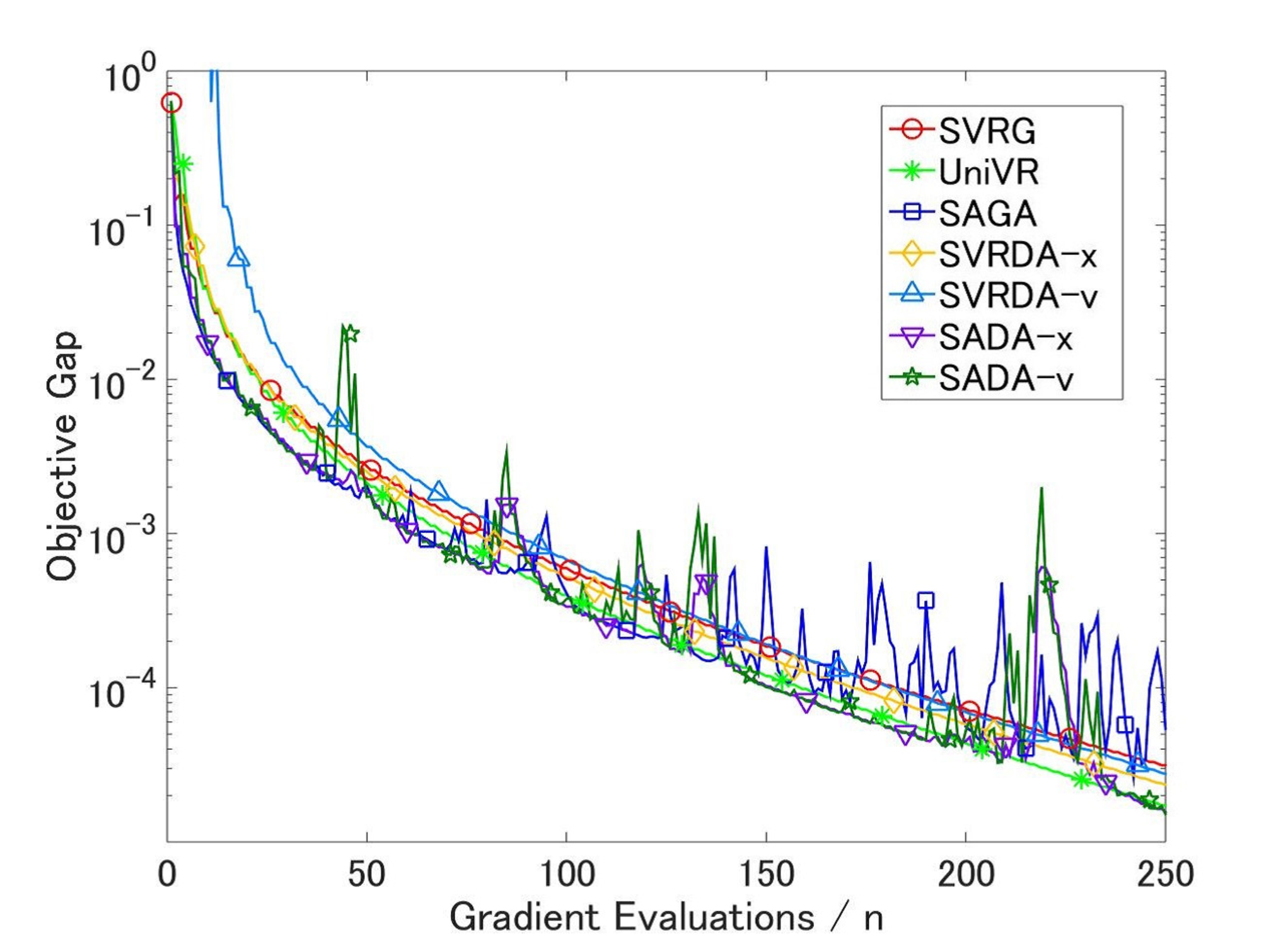
Refer to caption
Refer to caption
(a) λ1=10−4\lambda_{1}=10^{-4}, λ2=10−4\lambda_{2}=10^{-4}
Refer to caption
Refer to caption
(b) λ1=10−4\lambda_{1}=10^{-4}, λ2=0\lambda_{2}=0
Figure 2: Comparison of different methods on Reuters-21578 data set

Figures 2a and 2b show the comparison of different methods on the Reuters-21578 data set for different setups of λ1\lambda_{1} and λ2\lambda_{2} (the strongly convex case λ2=10−4>0\lambda_{2}=10^{-4}>0 (Figure 2a) and the non-strongly convex case λ2=0\lambda_{2}=0 (Figure 2b)). For a strongly convex regularizer, SVRG type algorithms (SVRG, UniVR, SVRDA-x, and SVRDA-v) show nice convergence behavior whereas SAGA type algorithms (SAGA, SADA-x, and SADA-v) show a slightly unstable behavior. Note that the sparsity pattern of the output solution of SVRG is poor. For a non-strongly convex regularizer, SVRDA-x and SADA-x converge more quickly but a bit more unstably than the other methods. Observe that, when a new stage starts, SVRDA-x and SADA-x lead to a sharp increase in the objective gap followed by a quick drop. This behavior can also be seen in the Multi-stage ORDA [2]. We can see that the sparsity recovery performances of SVRDA-x and SADA-x are very nice whereas that of UniVR is unstable and poor and that of SAGA is quite poor.

Refer to caption
Refer to caption
(a) λ1=10−4\lambda_{1}=10^{-4}, λ2=10−4\lambda_{2}=10^{-4}
Refer to caption
Refer to caption
(b) λ1=10−4\lambda_{1}=10^{-4}, λ2=0\lambda_{2}=0
Figure 3: Comparison of different methods on sido0 data set

Figures 3a and 3b show the comparison of different methods on the sido0 data set for different setups of λ1\lambda_{1} and λ2\lambda_{2} (the strongly convex case λ2=10−4>0\lambda_{2}=10^{-4}>0 (Figure 3a) and the non-strongly convex case λ2=0\lambda_{2}=0 (Figure 3b)). For a strongly convex regularizer, the performances of SAGA, SADA-x, and SADA-v are among the best. Especially, SADA-v shows the best sparsity recovery performance. Note that the sparsity recovery performance of SVRG is very poor. We can see that the convergence of the NNZs of SVRDA-v (respectively SADA-v) is superior to SVRDA-x (respectively SADA-x). For a non-strongly convex regularizer, SVRDA-x and SADA-x outperform both UniVR and SAGA. Especially, SVRDA-x and SADA-x show nice sparsity recovery performances though the solutions of UniVR and SAGA are not sparse at all.

7 Conclusion and future work

In this paper, we proposed two stochastic gradient methods for regularized empirical risk minimization problems: SVRDA and SADA. We have shown that SVRDA and SADA achieve O⁡((n+L¯μ)​log​1ε)O\left(\left(n+\frac{\bar{L}}{\mu}\right)\mathrm{log}\frac{1}{\varepsilon}\right) and O⁡((n+Lmaxμ)​log​1ε)O\left(\left(n+\frac{L_{\mathrm{max}}}{\mu}\right)\mathrm{log}\frac{1}{\varepsilon}\right)complexity, respectively, for a strongly convex regularizer and O⁡(n​log​1ε+L¯ε)O\left(n\mathrm{log}\frac{1}{\varepsilon}+\frac{\bar{L}}{\varepsilon}\right) and O⁡(n​log​1ε+Lmaxε)O\left(n\mathrm{log}\frac{1}{\varepsilon}+\frac{L_{\mathrm{max}}}{\varepsilon}\right) complexity, respectively, for a non-strongly convex regularizer.

In numerical experiments, our methods led to better sparsity recovery than the existing methods for sparsity-inducing regularizers and showed nice convergence behaviors, especially for non-strongly convex regularizers.

An interesting future work is to extend our methods to the alternating directional multiplier method (ADMM) framework. In this paper, we assumed that the proximal mapping of RR can be efficiently computed. However, for structured regularization problems (for example, overlapped group lasso, graph lasso, etc.), this assumption is generally not satisfied and our methods cannot be directly applied. In contrast, ADMM can be applied to these problems without this assumption. Suzuki [18] has proposed regularized dual averaging-ADMM (RDA-ADMM), which is RDA [20] for ADMM in an online setting. Furthermore, Suzuki [19] has proposed stochastic dual coordinate ascent-ADMM (SDCA-ADMM), which is SDCA [16, 15] for ADMM in regularized an empirical risk minimization setting, and has shown that it converges exponentially for a strongly convex regularizer. Applying SVRDA to the ADMM framework and showing linear convergence for a strongly convex regularizer would be promising future work.

Acknowledgement

This work was partially supported by MEXT Kakenhi (25730013, 25120012, and 26280009), JST-PRESTO and JST-CREST.

References

  • [1] Z. Allen-Zhu and Y. Yuan. Univr: A universal variance reduction framework for proximal stochastic gradient method. arXiv preprint arXiv:1506.01972, 2015.
  • [2] X. Chen, Q. Lin, and J. Pena. Optimal regularized dual averaging methods for stochastic optimization. In Advances in Neural Information Processing Systems, pages 395–403, 2012.
  • [3] A. Cotter, O. Shamir, N. Srebro, and K. Sridharan. Better mini-batch algorithms via accelerated gradient methods. In Advances in neural information processing systems, pages 1647–1655, 2011.
  • [4] A. Defazio, F. Bach, and S. Lacoste-Julien. Saga: A fast incremental gradient method with support for non-strongly convex composite objectives. In Advances in Neural Information Processing Systems, pages 1646–1654, 2014.
  • [5] O. Dekel, R. Gilad-Bachrach, O. Shamir, and L. Xiao. Optimal distributed online prediction using mini-batches. The Journal of Machine Learning Research, 13(1):165–202, 2012.
  • [6] E. Hazan, A. Agarwal, and S. Kale. Logarithmic regret algorithms for online convex optimization. Machine Learning, 69(2-3):169–192, 2007.
  • [7] R. Johnson and T. Zhang. Accelerating stochastic gradient descent using predictive variance reduction. In Advances in Neural Information Processing Systems, pages 315–323, 2013.
  • [8] Y. Nesterov. Primal-dual subgradient methods for convex problems. Mathematical programming, 120(1):221–259, 2009.
  • [9] Y. Nesterov. Introductory lectures on convex optimization: A basic course, volume 87. Springer Science & Business Media, 2013.
  • [10] A. Nitanda. Stochastic proximal gradient descent with acceleration techniques. In Advances in Neural Information Processing Systems, pages 1574–1582, 2014.
  • [11] N. L. Roux, M. Schmidt, and F. R. Bach. A stochastic gradient method with an exponential convergence _rate for finite training sets. In Advances in Neural Information Processing Systems, pages 2663–2671, 2012.
  • [12] M. Schmidt, N. L. Roux, and F. Bach. Minimizing finite sums with the stochastic average gradient. arXiv preprint arXiv:1309.2388, 2013.
  • [13] M. Schmidt, R. Babanezhad, M. O. Ahmed, A. Defazio, A. Clifton, and A. Sarkar. Non-uniform stochastic average gradient method for training conditional random fields. arXiv preprint arXiv:1504.04406, 2015.
  • [14] S. Shalev-Shwartz and Y. Singer. Logarithmic regret algorithms for strongly convex repeated games. The Hebrew University, 2007.
  • [15] S. Shalev-Shwartz and T. Zhang. Accelerated mini-batch stochastic dual coordinate ascent. In Advances in Neural Information Processing Systems, pages 378–385, 2013a.
  • [16] S. Shalev-Shwartz and T. Zhang. Stochastic dual coordinate ascent methods for regularized loss. The Journal of Machine Learning Research, 14(1):567–599, 2013b.
  • [17] Y. Singer and J. C. Duchi. Efficient learning using forward-backward splitting. In Advances in Neural Information Processing Systems, pages 495–503, 2009.
  • [18] T. Suzuki. Dual averaging and proximal gradient descent for online alternating direction multiplier method. In Proceedings of the 30th International Conference on Machine Learning (ICML-13), pages 392–400, 2013.
  • [19] T. Suzuki. Stochastic dual coordinate ascent with alternating direction method of multipliers. In Proceedings of the 31st International Conference on Machine Learning (ICML-14), pages 736–744, 2014.
  • [20] L. Xiao. Dual averaging method for regularized stochastic learning and online optimization. In Advances in Neural Information Processing Systems, pages 2116–2124, 2009.
  • [21] L. Xiao and T. Zhang. A proximal stochastic gradient method with progressive variance reduction. SIAM Journal on Optimization, 24(4):2057–2075, 2014.

Appendix

A Proof of Theorem 5.1

In this section, we give the proof of Theorem 5.1. First we prove the following two easy lemmas.

Lemma A.1.
g¯t=1t​∑τ=1tgτ​(t≥1).\bar{g}_{t}=\frac{1}{t}\sum_{\tau=1}^{t}g_{\tau}\ (t\geq 1).
Proof.

For t=1t=1, g¯1=g1=11​∑τ=11gτ\bar{g}_{1}=g_{1}=\frac{1}{1}\sum_{\tau=1}^{1}g_{\tau}.
Assume that the claim holds for some t≥1t\geq 1. Then

g¯t+1\displaystyle\bar{g}_{t+1} =(1−1t+1)​g¯t+1t+1​gt+1​(by the definition)\displaystyle=\left(1-\frac{1}{t+1}\right)\bar{g}_{t}+\frac{1}{t+1}g_{t+1}\ \text{(by the definition)}
=(1−1t+1)​1t​∑τ=1tgτ+1t+1​gt+1​(by the assumption of the induction)\displaystyle=\left(1-\frac{1}{t+1}\right)\frac{1}{t}\sum_{\tau=1}^{t}g_{\tau}+\frac{1}{t+1}g_{t+1}\ \text{(by the assumption of the induction)}
=1t+1​∑τ=1t+1gτ.\displaystyle=\frac{1}{t+1}\sum_{\tau=1}^{t+1}g_{\tau}.

This finishes the proof for Lemma A.1. ∎

Lemma A.2.

For every xx, u∈ℝdu\in\mathbb{R}^{d},

F⁡(u)+⟨∇F​(u),x−u⟩+R⁡(x)≤P⁡(x)−12​L¯​1n​∑i=1n1n​qi​‖∇fi​(x)−∇fi​(u)‖2.F(u)+\langle\nabla F(u),x-u\rangle+R(x)\leq P(x)-\frac{1}{2\bar{L}}\frac{1}{n}\sum_{i=1}^{n}\frac{1}{nq_{i}}||\nabla f_{i}(x)-\nabla f_{i}(u)||^{2}.
Proof.

Since fif_{i} is LiL_{i}-smooth, we have (see [9])

fi​(u)+⟨∇fi​(u),x−u⟩≤fi​(x)−12​Li​‖∇fi​(x)−∇fi​(u)‖2.f_{i}(u)+\langle\nabla f_{i}(u),x-u\rangle\leq f_{i}(x)-\frac{1}{2L_{i}}||\nabla f_{i}(x)-\nabla f_{i}(u)||^{2}.

Summing this inequality from i=1i=1 to nn and dividing it by nn results in

F⁡(u)+⟨∇F​(u),x−u⟩≤F⁡(x)−12​L¯​1n​∑i=1n1n​qi​‖∇fi​(x)−∇fi​(u)‖2.F(u)+\langle\nabla F(u),x-u\rangle\leq F(x)-\frac{1}{2\bar{L}}\frac{1}{n}\sum_{i=1}^{n}\frac{1}{nq_{i}}||\nabla f_{i}(x)-\nabla f_{i}(u)||^{2}.

Adding R⁡(x)R(x) gives the desired result. ∎

Next we prove the following main lemma.

Lemma A.3.

For the ssth stage of SVRDA,

𝔼⁡[P⁡(xms)−P⁡(x∗)]+η+ms​μ2​ms​𝔼​‖vms−x∗‖2\displaystyle\mathbb{E}[P({x}_{m_{s}})-P(x_{*})]+\frac{\eta+m_{s}\mu}{2m_{s}}\mathbb{E}||{v}_{m_{s}}-x_{*}||^{2}
≤\displaystyle\leq 12​ms​∑t=1ms[tη​t−L¯​𝔼​‖gt−∇F​(ut−1)‖2−1L¯​𝔼​[1n​∑i=1n1n​qi​‖∇fi​(ut−1)−∇fi​(x∗)‖2]]\displaystyle\frac{1}{2m_{s}}\sum_{t=1}^{m_{s}}\left[\frac{t}{\eta t-\bar{L}}\mathbb{E}||g_{t}-\nabla F(u_{t-1})||^{2}-\frac{1}{\bar{L}}\mathbb{E}\left[\frac{1}{n}\sum_{i=1}^{n}\frac{1}{nq_{i}}||\nabla f_{i}(u_{t-1})-\nabla f_{i}(x_{*})||^{2}\right]\right]
+η2​ms​‖v0−x∗‖2,\displaystyle+\frac{\eta}{2m_{s}}||{v}_{0}-x_{*}||^{2},

where the expectations are conditioned on all previous stages.

Proof.

First note that ut=(1−1t+1)​xt+1t+1​vtu_{t}=\left(1-\frac{1}{t+1}\right)x_{t}+\frac{1}{t+1}v_{t} for t≥0t\geq 0 by the definition of u0u_{0}. We define

ℓt​(x)\displaystyle\ell_{t}(x) =F⁡(ut−1)+⟨∇F​(ut−1),x−ut−1⟩+R⁡(x),\displaystyle=F(u_{t-1})+\langle\nabla F(u_{t-1}),x-u_{t-1}\rangle+R(x),
ℓ^t​(x)\displaystyle\hat{\ell}_{t}(x) =F⁡(ut−1)+⟨gt,x−ut−1⟩+R⁡(x).\displaystyle=F(u_{t-1})+\langle g_{t},x-u_{t-1}\rangle+R(x).

Observe that ℓt≤P\ell_{t}\leq P. For t≥1t\geq 1, by Lemma A.1, we have

∑τ=1tℓ^τ​(x)=\displaystyle\sum_{\tau=1}^{t}\hat{\ell}_{\tau}(x)= ∑τ=1tF⁡(ut−1)+∑τ=1t⟨gτ,x−uτ−1⟩+∑τ=1tR⁡(x)\displaystyle\sum_{\tau=1}^{t}F(u_{t-1})+\sum_{\tau=1}^{t}\langle g_{\tau},x-u_{\tau-1}\rangle+\sum_{\tau=1}^{t}R(x)
=\displaystyle= ⟨t​g¯t,x⟩+t​R​(x)+∑τ=1tF⁡(ut−1)−∑τ=1t⟨gτ,uτ−1⟩\displaystyle\langle t\bar{g}_{t},x\rangle+tR(x)+\sum_{\tau=1}^{t}F(u_{t-1})-\sum_{\tau=1}^{t}\langle g_{\tau},u_{\tau-1}\rangle

and thus we have vt=argminx∈ℝd​{∑τ=1tℓ^τ​(x)+η2​‖x−v0‖2}v_{t}=\underset{x\in\mathbb{R}^{d}}{\mathrm{argmin}\ }\left\{\sum_{\tau=1}^{t}\hat{\ell}_{\tau}(x)+\frac{\eta}{2}||x-v_{0}||^{2}\right\}.
Also note that xt=argminx∈ℝd​{ℓ^τ​(x)+η​t2​‖x−ut−1‖2}x_{t}=\underset{x\in\mathbb{R}^{d}}{\mathrm{argmin}\ }\left\{\hat{\ell}_{\tau}(x)+\frac{\eta t}{2}||x-u_{t-1}||^{2}\right\}. Since FF is L¯\bar{L}-smooth, we have (see [9])

F⁡(xt)≤F⁡(ut−1)+⟨∇F​(ut−1),xt−ut−1⟩+L¯2​‖xt−ut−1‖2,F(x_{t})\leq F(u_{t-1})+\langle\nabla F(u_{t-1}),x_{t}-u_{t-1}\rangle+\frac{\bar{L}}{2}||x_{t}-u_{t-1}||^{2},

and thus

P⁡(xt)≤\displaystyle P(x_{t})\leq ℓt​(xt)+L¯2​‖xt−ut−1‖2\displaystyle\ell_{t}(x_{t})+\frac{\bar{L}}{2}||x_{t}-u_{t-1}||^{2}
=\displaystyle= ℓ^t​(xt)+η​t2​‖xt−ut−1‖2−η​t−L¯2​‖xt−ut−1‖2−⟨gt−∇F​(ut−1),xt−ut−1⟩.\displaystyle\hat{\ell}_{t}(x_{t})+\frac{\eta t}{2}||x_{t}-u_{t-1}||^{2}-\frac{\eta t-\bar{L}}{2}||x_{t}-u_{t-1}||^{2}-\langle g_{t}-\nabla F(u_{t-1}),x_{t}-u_{t-1}\rangle.

Since xtx_{t} is the minimizer of ℓ^t​(x)+η​t2​‖x−ut−1‖2\hat{\ell}_{t}(x)+\frac{\eta t}{2}||x-u_{t-1}||^{2}, we have

ℓ^t​(xt)+\displaystyle\hat{\ell}_{t}(x_{t})+ η​t2​‖xt−ut−1‖2\displaystyle\frac{\eta t}{2}||x_{t}-u_{t-1}||^{2}
≤\displaystyle\leq ℓ^t​((1−1t)​xt−1+1t​vt)+η​t2​||(1−1t)​xt−1+1t​vt−ut−1||2\displaystyle\hat{\ell}_{t}\left(\left(1-\frac{1}{t}\right)x_{t-1}+\frac{1}{t}v_{t}\right)+\frac{\eta t}{2}\left|\left|\left(1-\frac{1}{t}\right)x_{t-1}+\frac{1}{t}v_{t}-u_{t-1}\right|\right|^{2}

and hence

P⁡(xt)≤\displaystyle P(x_{t})\leq ℓ^t​((1−1t)​xt−1+1t​vt)+η​t2​||(1−1t)​xt−1+1t​vt−ut−1||2\displaystyle\hat{\ell}_{t}\left(\left(1-\frac{1}{t}\right)x_{t-1}+\frac{1}{t}v_{t}\right)+\frac{\eta t}{2}\left|\left|\left(1-\frac{1}{t}\right)x_{t-1}+\frac{1}{t}v_{t}-u_{t-1}\right|\right|^{2}
−η​t−L¯2​‖xt−ut−1‖2−⟨gt−∇F​(ut−1),xt−ut−1⟩.\displaystyle-\frac{\eta t-\bar{L}}{2}||x_{t}-u_{t-1}||^{2}-\langle g_{t}-\nabla F(u_{t-1}),x_{t}-u_{t-1}\rangle.

Using the convexity of ℓ^t\hat{\ell}_{t} and the facts that (1−1t)​xt−1+1t​vt−ut−1=1t​(vt−vt−1)\left(1-\frac{1}{t}\right)x_{t-1}+\frac{1}{t}v_{t}-u_{t-1}=\frac{1}{t}(v_{t}-v_{t-1}) and

−η​t−L¯2​‖xt−ut−1‖2−\displaystyle-\frac{\eta t-\bar{L}}{2}||x_{t}-u_{t-1}||^{2}- ⟨gt−∇F​(ut−1),xt−ut−1⟩≤12​(η​t−L¯)​‖gt−∇F​(ut−1)‖2,\displaystyle\langle g_{t}-\nabla F(u_{t-1}),x_{t}-u_{t-1}\rangle\leq\frac{1}{2(\eta t-\bar{L})}||g_{t}-\nabla F(u_{t-1})||^{2},

we get

P⁡(xt)≤\displaystyle P(x_{t})\leq (1−1t)​ℓ^t​(xt−1)+1t​ℓ^t​(vt)+η2​t​‖vt−vt−1‖2+12​(η​t−L¯)​‖gt−∇F​(ut−1)‖2\displaystyle\left(1-\frac{1}{t}\right)\hat{\ell}_{t}(x_{t-1})+\frac{1}{t}\hat{\ell}_{t}(v_{t})+\frac{\eta}{2t}||v_{t}-v_{t-1}||^{2}+\frac{1}{2(\eta t-\bar{L})}||g_{t}-\nabla F(u_{t-1})||^{2}
=\displaystyle= (1−1t)​ℓt​(xt−1)+1t​ℓ^t​(vt)+η2​t​‖vt−vt−1‖2\displaystyle\left(1-\frac{1}{t}\right)\ell_{t}(x_{t-1})+\frac{1}{t}\hat{\ell}_{t}(v_{t})+\frac{\eta}{2t}||v_{t}-v_{t-1}||^{2}
+12​(η​t−L¯)​‖gt−∇F​(ut−1)‖2+(1−1t)​⟨gt−∇F​(ut−1),xt−1−ut−1⟩\displaystyle+\frac{1}{2(\eta t-\bar{L})}||g_{t}-\nabla F(u_{t-1})||^{2}+\left(1-\frac{1}{t}\right)\langle g_{t}-\nabla F(u_{t-1}),x_{t-1}-u_{t-1}\rangle
≤\displaystyle\leq (1−1t)​P​(xt−1)+1t​ℓ^t​(vt)+η2​t​‖vt−vt−1‖2\displaystyle\left(1-\frac{1}{t}\right)P(x_{t-1})+\frac{1}{t}\hat{\ell}_{t}(v_{t})+\frac{\eta}{2t}||v_{t}-v_{t-1}||^{2}
+12​(η​t−L¯)​‖gt−∇F​(ut−1)‖2+(1−1t)​⟨gt−∇F​(ut−1),xt−1−ut−1⟩.\displaystyle+\frac{1}{2(\eta t-\bar{L})}||g_{t}-\nabla F(u_{t-1})||^{2}+\left(1-\frac{1}{t}\right)\langle g_{t}-\nabla F(u_{t-1}),x_{t-1}-u_{t-1}\rangle.

Multiplying both sides of the above inequality by tt, we have

t​P​(xt)≤\displaystyle tP(x_{t})\leq (t−1)​P​(xt−1)+ℓ^t​(vt)+η2​‖vt−vt−1‖2\displaystyle(t-1)P(x_{t-1})+\hat{\ell}_{t}(v_{t})+\frac{\eta}{2}||v_{t}-v_{t-1}||^{2}
+t2​(η​t−L¯)​‖gt−∇F​(ut−1)‖2+(t−1)​⟨gt−∇F​(ut−1),xt−1−ut−1⟩.\displaystyle+\frac{t}{2(\eta t-\bar{L})}||g_{t}-\nabla F(u_{t-1})||^{2}+(t-1)\langle g_{t}-\nabla F(u_{t-1}),x_{t-1}-u_{t-1}\rangle.

By the fact that ∑τ=1t−1ℓ^τ​(x)+η2​‖x−v0‖2\sum_{\tau=1}^{t-1}\hat{\ell}_{\tau}(x)+\frac{\eta}{2}||x-v_{0}||^{2} is η\eta-strongly convex and vt−1v_{t-1} is the minimizer of ∑τ=1t−1ℓ^τ​(x)+η2​‖x−v0‖2\sum_{\tau=1}^{t-1}\hat{\ell}_{\tau}(x)+\frac{\eta}{2}||x-v_{0}||^{2} for t≥2t\geq 2, we have

∑τ=1t−1ℓ^τ​(vt−1)+η2​‖vt−1−v0‖2+η2​‖vt−vt−1‖2≤∑τ=1t−1ℓ^τ​(vt)+η2​‖vt−v0‖2\sum_{\tau=1}^{t-1}\hat{\ell}_{\tau}(v_{t-1})+\frac{\eta}{2}||v_{t-1}-v_{0}||^{2}+\frac{\eta}{2}||v_{t}-v_{t-1}||^{2}\leq\sum_{\tau=1}^{t-1}\hat{\ell}_{\tau}(v_{t})+\frac{\eta}{2}||v_{t}-v_{0}||^{2}

for t≥1t\geq 1 (and, for t=1t=1, we define ∑τ=10=0\sum_{\tau=1}^{0}=0). Using this inequality, we obtain

t​P​(xt)−∑τ=1tℓ^τ​(vt)−η2​‖vt−v0‖2\displaystyle tP(x_{t})-\sum_{\tau=1}^{t}\hat{\ell}_{\tau}(v_{t})-\frac{\eta}{2}||v_{t}-v_{0}||^{2}
≤\displaystyle\leq (t−1)​P​(xt−1)−∑τ=1t−1ℓ^τ​(vt−1)−η2​‖vt−1−v0‖2+t2​(η​t−L¯)​‖gt−∇F​(ut−1)‖2\displaystyle(t-1)P(x_{t-1})-\sum_{\tau=1}^{t-1}\hat{\ell}_{\tau}(v_{t-1})-\frac{\eta}{2}||v_{t-1}-v_{0}||^{2}+\frac{t}{2(\eta t-\bar{L})}||g_{t}-\nabla F(u_{t-1})||^{2}
+(t−1)​⟨gt−∇F​(ut−1),xt−1−ut−1⟩.\displaystyle+(t-1)\langle g_{t}-\nabla F(u_{t-1}),x_{t-1}-u_{t-1}\rangle.

Summing the above inequality from t=1t=1 to msm_{s} results in

ms​P​(xms)−\displaystyle m_{s}P(x_{m_{s}})- ∑t=1msℓ^t​(vms)−η2​‖vms−v0‖2\displaystyle\sum_{t=1}^{m_{s}}\hat{\ell}_{t}(v_{m_{s}})-\frac{\eta}{2}||v_{m_{s}}-v_{0}||^{2}
≤\displaystyle\leq ∑t=1mst2​(η​t−L¯)​‖gt−∇F​(ut−1)‖2\displaystyle\sum_{t=1}^{m_{s}}\frac{t}{2(\eta t-\bar{L})}||g_{t}-\nabla F(u_{t-1})||^{2}
+∑t=1ms(t−1)⟨gt−∇F(ut−1),xt−1−ut−1⟩.\displaystyle+\sum_{t=1}^{m_{s}}(t-1)\langle g_{t}-\nabla F(u_{t-1}),x_{t-1}-u_{t-1}\rangle.

Using η+ms​μ\eta+m_{s}\mu-strongly convexity of the function ∑t=1msℓ^t​(x)+η2​‖x−v0‖2\sum_{t=1}^{m_{s}}\hat{\ell}_{t}(x)+\frac{\eta}{2}||x-v_{0}||^{2} and the optimality of vmsv_{m_{s}}, we have

∑t=1msℓ^t​(vms)+η2​‖vms−v0‖2≤∑t=1msℓ^t​(x∗)+η2​‖v0−x∗‖2−η+ms​μ2​‖vms−x∗‖2\sum_{t=1}^{m_{s}}\hat{\ell}_{t}(v_{m_{s}})+\frac{\eta}{2}||v_{m_{s}}-v_{0}||^{2}\leq\sum_{t=1}^{m_{s}}\hat{\ell}_{t}(x_{*})+\frac{\eta}{2}||v_{0}-x_{*}||^{2}-\frac{\eta+m_{s}\mu}{2}||v_{m_{s}}-x_{*}||^{2}

and hence

ms​P​(xms)\displaystyle m_{s}P(x_{m_{s}})
≤\displaystyle\leq ∑t=1msℓ^t​(x∗)+η2​‖v0−x∗‖2−η+ms​μ2​‖vms−x∗‖2\displaystyle\sum_{t=1}^{m_{s}}\hat{\ell}_{t}(x_{*})+\frac{\eta}{2}||v_{0}-x_{*}||^{2}-\frac{\eta+m_{s}\mu}{2}||v_{m_{s}}-x_{*}||^{2}
+∑t=1mst2​(η​t−L¯)||gt−∇F(ut−1)||2+∑t=1ms(t−1)⟨gt−∇F(ut−1),xt−1−ut−1⟩\displaystyle+\sum_{t=1}^{m_{s}}\frac{t}{2(\eta t-\bar{L})}||g_{t}-\nabla F(u_{t-1})||^{2}+\sum_{t=1}^{m_{s}}(t-1)\langle g_{t}-\nabla F(u_{t-1}),x_{t-1}-u_{t-1}\rangle
=\displaystyle= ∑t=1msℓt​(x∗)+η2​‖v0−x∗‖2−η+ms​μ2​‖vms−x∗‖2\displaystyle\sum_{t=1}^{m_{s}}\ell_{t}(x_{*})+\frac{\eta}{2}||v_{0}-x_{*}||^{2}-\frac{\eta+m_{s}\mu}{2}||v_{m_{s}}-x_{*}||^{2}
+∑t=1mst2​(η​t−L¯)||gt−∇F(ut−1)||2+∑t=1ms(t−1)⟨gt−∇F(ut−1),xt−1−ut−1⟩\displaystyle+\sum_{t=1}^{m_{s}}\frac{t}{2(\eta t-\bar{L})}||g_{t}-\nabla F(u_{t-1})||^{2}+\sum_{t=1}^{m_{s}}(t-1)\langle g_{t}-\nabla F(u_{t-1}),x_{t-1}-u_{t-1}\rangle
+∑t=1ms⟨gt−∇F(ut−1),x∗−ut−1⟩.\displaystyle+\sum_{t=1}^{m_{s}}\langle g_{t}-\nabla F(u_{t-1}),x_{*}-u_{t-1}\rangle.

By Lemma A.2 with x=x∗x=x_{*} and u=ut−1u=u_{t-1}, we have

ℓt​(x∗)≤P⁡(x∗)−12​L¯​1n​∑i=1n1n​qi​‖∇fi​(x∗)−∇fi​(ut−1)‖2.\ell_{t}(x_{*})\leq P(x_{*})-\frac{1}{2\bar{L}}\frac{1}{n}\sum_{i=1}^{n}\frac{1}{nq_{i}}||\nabla f_{i}(x_{*})-\nabla f_{i}(u_{t-1})||^{2}.

Applying this inequality to the above inequality yields

ms​P​(xms)\displaystyle m_{s}P(x_{m_{s}})
≤\displaystyle\leq ms​P​(x∗)+η2​‖v0−x∗‖2−η+ms​μ2​‖vms−x∗‖2\displaystyle m_{s}P(x_{*})+\frac{\eta}{2}||v_{0}-x_{*}||^{2}-\frac{\eta+m_{s}\mu}{2}||v_{m_{s}}-x_{*}||^{2}
+12∑t=1ms[tη​t−L¯||gt−∇F(ut−1)||2−1L¯1n∑i=1n1n​qi||∇fi(x∗)−∇fi(ut−1)||2]\displaystyle+\frac{1}{2}\sum_{t=1}^{m_{s}}\left[\frac{t}{\eta t-\bar{L}}||g_{t}-\nabla F(u_{t-1})||^{2}-\frac{1}{\bar{L}}\frac{1}{n}\sum_{i=1}^{n}\frac{1}{nq_{i}}||\nabla f_{i}(x_{*})-\nabla f_{i}(u_{t-1})||^{2}\right]
+∑t=1ms(t−1)⟨gt−∇F(ut−1),xt−1−ut−1⟩+∑t=1ms⟨gt−∇F(ut−1),x∗−ut−1⟩.\displaystyle+\sum_{t=1}^{m_{s}}(t-1)\langle g_{t}-\nabla F(u_{t-1}),x_{t-1}-u_{t-1}\rangle+\sum_{t=1}^{m_{s}}\langle g_{t}-\nabla F(u_{t-1}),x_{*}-u_{t-1}\rangle.

Dividing this inequality by msm_{s} results in

P⁡(xms)\displaystyle P(x_{m_{s}})
≤\displaystyle\leq P⁡(x∗)+η2​ms​‖v0−x∗‖2−η+ms​μ2​ms​‖vms−x∗‖2\displaystyle P(x_{*})+\frac{\eta}{2m_{s}}||v_{0}-x_{*}||^{2}-\frac{\eta+m_{s}\mu}{2m_{s}}||v_{m_{s}}-x_{*}||^{2}
+12​ms∑t=1ms[tη​t−L¯||gt−∇F(ut−1)||2−1L¯1n∑i=1n1n​qi||∇fi(x∗)−∇fi(ut−1)||2]\displaystyle+\frac{1}{2m_{s}}\sum_{t=1}^{m_{s}}\left[\frac{t}{\eta t-\bar{L}}||g_{t}-\nabla F(u_{t-1})||^{2}-\frac{1}{\bar{L}}\frac{1}{n}\sum_{i=1}^{n}\frac{1}{nq_{i}}||\nabla f_{i}(x_{*})-\nabla f_{i}(u_{t-1})||^{2}\right]
+1ms∑t=1ms(t−1)⟨gt−∇F(ut−1),xt−1−ut−1⟩+1ms∑t=1ms⟨gt−∇F(ut−1),x∗−ut−1⟩.\displaystyle+\frac{1}{m_{s}}\sum_{t=1}^{m_{s}}(t-1)\langle g_{t}-\nabla F(u_{t-1}),x_{t-1}-u_{t-1}\rangle+\frac{1}{m_{s}}\sum_{t=1}^{m_{s}}\langle g_{t}-\nabla F(u_{t-1}),x_{*}-u_{t-1}\rangle.

Taking the expectation on both sides yields

𝔼⁡[P⁡(xms)−P⁡(x∗)]+η+ms​μ2​ms​𝔼​‖vms−x∗‖2\displaystyle\mathbb{E}[P({x}_{m_{s}})-P(x_{*})]+\frac{\eta+m_{s}\mu}{2m_{s}}\mathbb{E}||{v}_{m_{s}}-x_{*}||^{2}
≤\displaystyle\leq 12​ms​∑t=1ms[tη​t−L¯​𝔼​‖gt−∇F​(ut−1)‖2−1L¯​𝔼​[1n​∑i=1n1n​qi​‖∇fi​(x∗)−∇fi​(ut−1)‖2]]\displaystyle\frac{1}{2m_{s}}\sum_{t=1}^{m_{s}}\left[\frac{t}{\eta t-\bar{L}}\mathbb{E}||g_{t}-\nabla F(u_{t-1})||^{2}-\frac{1}{\bar{L}}\mathbb{E}\left[\frac{1}{n}\sum_{i=1}^{n}\frac{1}{nq_{i}}||\nabla f_{i}(x_{*})-\nabla f_{i}(u_{t-1})||^{2}\right]\right]
+η2​ms​‖v0−x∗‖2.\displaystyle+\frac{\eta}{2m_{s}}||{v}_{0}-x_{*}||^{2}.

Here we used the fact that 𝔼⁡[gt−∇F​(ut−1)]=0\mathbb{E}[g_{t}-\nabla F(u_{t-1})]=0 for t=1,…,mst=1,\ldots,m_{s}. This finishes the proof of Lemma A.3. ∎

Now we need the following lemma.

Lemma A.4.

For every x∈ℝdx\in\mathbb{R}^{d},

1n​∑i=1n1n​qi​‖∇fi​(x)−∇fi​(x∗)‖2≤2​L¯​(P⁡(x)−P⁡(x∗)−μ2​‖x−x∗‖2).\frac{1}{n}\sum_{i=1}^{n}\frac{1}{nq_{i}}||\nabla f_{i}(x)-\nabla f_{i}(x_{*})||^{2}\leq 2\bar{L}(P(x)-P(x_{*})-\frac{\mu}{2}||x-x_{*}||^{2}).
Proof.

From the argument of the proof of Lemma A.2, we have

1n​∑i=1n1n​qi​‖∇fi​(x)−∇fi​(x∗)‖2≤2​L¯​(F⁡(x)−⟨∇F​(x∗),x−x∗⟩−F⁡(x∗)).\frac{1}{n}\sum_{i=1}^{n}\frac{1}{nq_{i}}||\nabla f_{i}(x)-\nabla f_{i}(x_{*})||^{2}\leq 2\bar{L}(F(x)-\langle\nabla F(x_{*}),x-x_{*}\rangle-F(x_{*})).

By the optimality of x∗x_{*}, there exists ξ∗∈∂R⁡(x∗)\xi_{*}\in\partial R(x_{*}) such that ∇F​(x∗)+ξ∗\nabla F(x_{*})+\xi_{*}. Then using μ\mu-strong convexity of RR, we get

−⟨∇F​(x∗),x−x∗⟩=⟨ξ∗,x−x∗⟩≤R⁡(x)−R⁡(x∗)−μ2​‖x−x∗‖2-\langle\nabla F(x_{*}),x-x_{*}\rangle=\langle\xi_{*},x-x_{*}\rangle\leq R(x)-R(x_{*})-\frac{\mu}{2}||x-x_{*}||^{2}

and hence

1n​∑i=1n1n​qi​‖∇fi​(x)−∇fi​(x∗)‖2≤2​L¯​(P⁡(x)−P⁡(x∗)−μ2​‖x−x∗‖2).\frac{1}{n}\sum_{i=1}^{n}\frac{1}{nq_{i}}||\nabla f_{i}(x)-\nabla f_{i}(x_{*})||^{2}\leq 2\bar{L}(P(x)-P(x_{*})-\frac{\mu}{2}||x-x_{*}||^{2}).

∎

Proof of Theorem 5.1.

We bound the term 𝔼​‖gt−∇F​(ut−1)‖2\mathbb{E}||g_{t}-\nabla F(u_{t-1})||^{2}:

𝔼​‖gt−∇F​(ut−1)‖2\displaystyle\mathbb{E}||g_{t}-\nabla F(u_{t-1})||^{2}
=\displaystyle= 𝔼[𝔼it[||(∇fit(ut−1)−∇fit(x0))/nqit+∇F(x0)−∇F(ut−1)||2|i1,…,it−1]]\displaystyle\mathbb{E}\left[\mathbb{E}_{i_{t}}\left[||(\nabla f_{i_{t}}(u_{t-1})-\nabla f_{i_{t}}(x_{0}))/nq_{i_{t}}+\nabla F(x_{0})-\nabla F(u_{t-1})||^{2}|i_{1},\ldots,i_{t-1}\right]\right]
≤\displaystyle\leq 𝔼[𝔼it[||(∇fit(ut−1)−∇fit(x0))/nqit||2|i1,…,it−1]]\displaystyle\mathbb{E}\left[\mathbb{E}_{i_{t}}\left[||(\nabla f_{i_{t}}(u_{t-1})-\nabla f_{i_{t}}(x_{0}))/nq_{i_{t}}||^{2}|i_{1},\ldots,i_{t-1}\right]\right]
=\displaystyle= 𝔼⁡[1n​∑i=1n1n​qi​‖∇fi​(ut−1)−∇fi​(x0)‖2]\displaystyle\mathbb{E}\left[\frac{1}{n}\sum_{i=1}^{n}\frac{1}{nq_{i}}||\nabla f_{i}(u_{t-1})-\nabla f_{i}(x_{0})||^{2}\right]
≤\displaystyle\leq 3​𝔼​[1n​∑i=1n1n​qi​‖∇fi​(ut−1)−∇fi​(x∗)‖2]+32​[1n​∑i=1n1n​qi​‖∇fi​(x0)−∇fi​(x∗)‖2].\displaystyle 3\mathbb{E}\left[\frac{1}{n}\sum_{i=1}^{n}\frac{1}{nq_{i}}||\nabla f_{i}(u_{t-1})-\nabla f_{i}(x_{*})||^{2}\right]+\frac{3}{2}\left[\frac{1}{n}\sum_{i=1}^{n}\frac{1}{nq_{i}}||\nabla f_{i}(x_{0})-\nabla f_{i}(x_{*})||^{2}\right].

Combining this inequality with Lemme A.4, we get

𝔼​‖gt−∇F​(ut−1)‖2≤\displaystyle\mathbb{E}||g_{t}-\nabla F(u_{t-1})||^{2}\leq 3​𝔼​[1n​∑i=1n1n​qi​‖∇fi​(ut−1)−∇fi​(x∗)‖2]\displaystyle 3\mathbb{E}\left[\frac{1}{n}\sum_{i=1}^{n}\frac{1}{nq_{i}}||\nabla f_{i}(u_{t-1})-\nabla f_{i}(x_{*})||^{2}\right]
+3​L¯​(P⁡(x0)−P⁡(x∗)−μ2​‖x0−x∗‖2).\displaystyle+3\bar{L}(P(x_{0})-P(x_{*})-\frac{\mu}{2}||x_{0}-x_{*}||^{2}).

Since η=14​L¯\eta=\frac{1}{4\bar{L}}, using the inequality

tη​t−L¯≤13​L¯(∀t≥1),\frac{t}{\eta t-\bar{L}}\leq\frac{1}{3\bar{L}}\ \ \ \ (\forall t\geq 1), (8)

by Lemma A.3 we obtain

𝔼⁡[P⁡(xms)−P⁡(x∗)]+η+ms​μ2​ms​𝔼​‖vms−x∗‖2\displaystyle\mathbb{E}[P({x}_{m_{s}})-P(x_{*})]+\frac{\eta+m_{s}\mu}{2m_{s}}\mathbb{E}||{v}_{m_{s}}-x_{*}||^{2}
≤\displaystyle\leq 12​(P⁡(x0)−P⁡(x∗)−μ2​‖x0−x∗‖2)+η2​ms​‖v0−x∗‖2.\displaystyle\frac{1}{2}(P(x_{0})-P(x_{*})-\frac{\mu}{2}||x_{0}-x_{*}||^{2})+\frac{\eta}{2m_{s}}||{v}_{0}-x_{*}||^{2}.

Since xms=x~sx_{m_{s}}=\widetilde{x}_{s}, vms=v~sv_{m_{s}}=\widetilde{v}_{s}, x0=x~s−1x_{0}=\widetilde{x}_{s-1}, and v0=(1−α)​v~s−1+α​x~s−1v_{0}=(1-\alpha)\widetilde{v}_{s-1}+\alpha\widetilde{x}_{s-1}, we have

𝔼⁡[P⁡(x~s)−P⁡(x∗)]+η+ms​μ2​ms​𝔼​‖v~s−x∗‖2\displaystyle\mathbb{E}[P(\widetilde{x}_{s})-P(x_{*})]+\frac{\eta+m_{s}\mu}{2m_{s}}\mathbb{E}||\widetilde{v}_{s}-x_{*}||^{2}
≤\displaystyle\leq 12​(P⁡(x~s−1)−P⁡(x∗))+(α​η2​ms−μ4)​‖x~s−1−x∗‖2+(1−α)​η2​ms​‖v~s−1−x∗‖2.\displaystyle\frac{1}{2}(P(\widetilde{x}_{s-1})-P(x_{*}))+\left(\frac{\alpha\eta}{2m_{s}}-\frac{\mu}{4}\right)||\widetilde{x}_{s-1}-x_{*}||^{2}+\frac{(1-\alpha)\eta}{2m_{s}}||\widetilde{v}_{s-1}-x_{*}||^{2}.

Finally, taking expectations with respect to all previous stages gives the desired result. ∎

B Proof of Theorem 5.4

In this section, we give the proof of Theorem 5.4.

Lemma B.1.

For the ssth stage of SADA,

𝔼⁡[P⁡(xms)−P⁡(x∗)]+η+ms​μ2​ms​𝔼​‖vms−x∗‖2\displaystyle\mathbb{E}[P({x}_{m_{s}})-P(x_{*})]+\frac{\eta+m_{s}\mu}{2m_{s}}\mathbb{E}||{v}_{m_{s}}-x_{*}||^{2}
≤\displaystyle\leq 12​ms​∑t=1ms[tη​t−Lmax​𝔼​‖gt−∇F​(ut−1)‖2−1Lmax​𝔼​[1n​∑i=1n‖∇fi​(ut−1)−∇fi​(x∗)‖2]]\displaystyle\frac{1}{2m_{s}}\sum_{t=1}^{m_{s}}\left[\frac{t}{\eta t-L_{\mathrm{max}}}\mathbb{E}||g_{t}-\nabla F(u_{t-1})||^{2}-\frac{1}{L_{\mathrm{max}}}\mathbb{E}\left[\frac{1}{n}\sum_{i=1}^{n}||\nabla f_{i}(u_{t-1})-\nabla f_{i}(x_{*})||^{2}\right]\right]
+η2​ms​‖v0−x∗‖2.\displaystyle+\frac{\eta}{2m_{s}}||{v}_{0}-x_{*}||^{2}.

The proof of Lemma B.1 is identical to the proof of Lemma A.3 and we omit it.

Proof of Theorem 5.4.

First we bound the term 𝔼​‖gt−∇f​(ut−1)‖2\mathbb{E}||g_{t}-\nabla f(u_{t-1})||^{2}:

𝔼​‖gt−∇F​(ut−1)‖2=\displaystyle\mathbb{E}||g_{t}-\nabla F(u_{t-1})||^{2}= 𝔼[𝔼it[||∇fit(ut−1)−∇fit(ϕitt−1)+1n∑i=1n∇fi(ϕit−1)−∇F(ut−1)||2|i1,…,it−1]]\displaystyle\mathbb{E}\left[\mathbb{E}_{i_{t}}\left[||\nabla f_{i_{t}}(u_{t-1})-\nabla f_{i_{t}}(\phi_{i_{t}}^{t-1})+\frac{1}{n}\sum_{i=1}^{n}\nabla f_{i}(\phi_{i}^{t-1})-\nabla F(u_{t-1})||^{2}|i_{1},\ldots,i_{t-1}\right]\right]
≤\displaystyle\leq 𝔼[𝔼it[||∇fit(ut−1)−∇fit(ϕitt−1)||2|i1,…,it−1]]\displaystyle\mathbb{E}\left[\mathbb{E}_{i_{t}}\left[||\nabla f_{i_{t}}(u_{t-1})-\nabla f_{i_{t}}(\phi_{i_{t}}^{t-1})||^{2}|i_{1},\ldots,i_{t-1}\right]\right]
=\displaystyle= 𝔼⁡[1n​∑i=1n‖(∇fi​(ut−1)−∇fi​(ϕit−1))‖2]\displaystyle\mathbb{E}\left[\frac{1}{n}\sum_{i=1}^{n}||(\nabla f_{i}(u_{t-1})-\nabla f_{i}(\phi_{i}^{t-1}))||^{2}\right]
≤\displaystyle\leq 2​𝔼​[1n​∑i=1n‖(∇fi​(ut−1)−∇fi​(x∗))‖2]+2​𝔼​[1n​∑i=1n‖(∇fi​(ϕit−1)−∇fi​(x∗))‖2].\displaystyle 2\mathbb{E}\left[\frac{1}{n}\sum_{i=1}^{n}||(\nabla f_{i}(u_{t-1})-\nabla f_{i}(x_{*}))||^{2}\right]+2\mathbb{E}\left[\frac{1}{n}\sum_{i=1}^{n}||(\nabla f_{i}(\phi_{i}^{t-1})-\nabla f_{i}(x_{*}))||^{2}\right].

Next we bound the term 𝔼⁡[1n​∑i=1n‖(∇fi​(ϕit−1)−∇fi​(x∗))‖2]\mathbb{E}\left[\frac{1}{n}\sum_{i=1}^{n}||(\nabla f_{i}(\phi_{i}^{t-1})-\nabla f_{i}(x_{*}))||^{2}\right] for t≥1t\geq 1:

𝔼⁡[1n​∑i=1n‖(∇fi​(ϕit−1)−∇fi​(x∗))‖2]\displaystyle\mathbb{E}\left[\frac{1}{n}\sum_{i=1}^{n}||(\nabla f_{i}(\phi_{i}^{t-1})-\nabla f_{i}(x_{*}))||^{2}\right]
=\displaystyle= 𝔼[𝔼it−1[1n∑i=1n||(∇fi(ϕit−1)−∇fi(x∗))||2|i1,…,it−2]]\displaystyle\mathbb{E}\left[\mathbb{E}_{i_{t-1}}\left[\frac{1}{n}\sum_{i=1}^{n}||(\nabla f_{i}(\phi_{i}^{t-1})-\nabla f_{i}(x_{*}))||^{2}|i_{1},\ldots,i_{t-2}\right]\right]
=\displaystyle= 𝔼[1n∑i=1n𝔼it−1[||(∇fi(ϕit−1)−∇fi(x∗))||2|i1,…,it−2]]\displaystyle\mathbb{E}\left[\frac{1}{n}\sum_{i=1}^{n}\mathbb{E}_{i_{t-1}}\left[||(\nabla f_{i}(\phi_{i}^{t-1})-\nabla f_{i}(x_{*}))||^{2}|i_{1},\ldots,i_{t-2}\right]\right]
=\displaystyle= 𝔼⁡[1n​∑i=1n[1n​‖(∇fi​(ut−2)−∇fi​(x∗))‖2+(1−1n)​‖(∇fi​(ϕit−2)−∇fi​(x∗))‖2]]\displaystyle\mathbb{E}\left[\frac{1}{n}\sum_{i=1}^{n}\left[\frac{1}{n}||(\nabla f_{i}(u_{t-2})-\nabla f_{i}(x_{*}))||^{2}+\left(1-\frac{1}{n}\right)||(\nabla f_{i}(\phi_{i}^{t-2})-\nabla f_{i}(x_{*}))||^{2}\right]\right]
=\displaystyle= 1n​𝔼​[1n​∑i=1n‖(∇fi​(ut−2)−∇fi​(x∗))‖2]+(1−1n)​𝔼​[1n​∑i=1n‖(∇fi​(ϕit−2)−∇fi​(x∗))‖2]\displaystyle\frac{1}{n}\mathbb{E}\left[\frac{1}{n}\sum_{i=1}^{n}||(\nabla f_{i}(u_{t-2})-\nabla f_{i}(x_{*}))||^{2}\right]+\left(1-\frac{1}{n}\right)\mathbb{E}\left[\frac{1}{n}\sum_{i=1}^{n}||(\nabla f_{i}(\phi_{i}^{t-2})-\nabla f_{i}(x_{*}))||^{2}\right]
=\displaystyle= ⋯\displaystyle\cdots
=\displaystyle= ∑j=1t−11n​(1−1n)t−1−j​𝔼​[1n​∑i=1n‖(∇fi​(uj−1)−∇fi​(x∗))‖2]\displaystyle\sum_{j=1}^{t-1}\frac{1}{n}\left(1-\frac{1}{n}\right)^{t-1-j}\mathbb{E}\left[\frac{1}{n}\sum_{i=1}^{n}||(\nabla f_{i}(u_{j-1})-\nabla f_{i}(x_{*}))||^{2}\right]
+(1−1n)t−1​[1n​∑i=1n‖(∇fi​(ϕi0)−∇fi​(x∗))‖2].\displaystyle+\left(1-\frac{1}{n}\right)^{t-1}\left[\frac{1}{n}\sum_{i=1}^{n}||(\nabla f_{i}(\phi_{i}^{0})-\nabla f_{i}(x_{*}))||^{2}\right].

Here we defined ∑j=10=0\sum_{j=1}^{0}=0 for t=1t=1.

Using these inequalities and the definition of η\eta, we have

∑t=1ms[tη​t−Lmax​𝔼​‖gt−∇F​(ut−1)‖2−1Lmax​𝔼​[1n​∑i=1n‖∇fi​(ut−1)−∇fi​(x∗)‖2]]\displaystyle\sum_{t=1}^{m_{s}}\left[\frac{t}{\eta t-L_{\mathrm{max}}}\mathbb{E}||g_{t}-\nabla F(u_{t-1})||^{2}-\frac{1}{L_{\mathrm{max}}}\mathbb{E}\left[\frac{1}{n}\sum_{i=1}^{n}||\nabla f_{i}(u_{t-1})-\nabla f_{i}(x_{*})||^{2}\right]\right]
=\displaystyle= ∑t=1ms[12​Lmax​𝔼​[1n​∑i=1n‖(∇fi​(ϕit−1)−∇fi​(x∗))‖2]−12​Lmax​𝔼​[1n​∑i=1n‖∇fi​(ut−1)−∇fi​(x∗)‖2]]\displaystyle\sum_{t=1}^{m_{s}}\left[\frac{1}{2L_{\mathrm{max}}}\mathbb{E}\left[\frac{1}{n}\sum_{i=1}^{n}||(\nabla f_{i}(\phi_{i}^{t-1})-\nabla f_{i}(x_{*}))||^{2}\right]-\frac{1}{2L_{\mathrm{max}}}\mathbb{E}\left[\frac{1}{n}\sum_{i=1}^{n}||\nabla f_{i}(u_{t-1})-\nabla f_{i}(x_{*})||^{2}\right]\right]
=\displaystyle= 12​Lmax​∑t=1ms[∑j=1t−11n​(1−1n)t−1−j​𝔼​[1n​∑i=1n‖(∇fi​(uj−1)−∇fi​(x∗))‖2]]\displaystyle\frac{1}{2L_{\mathrm{max}}}\sum_{t=1}^{m_{s}}\left[\sum_{j=1}^{t-1}\frac{1}{n}\left(1-\frac{1}{n}\right)^{t-1-j}\mathbb{E}\left[\frac{1}{n}\sum_{i=1}^{n}||(\nabla f_{i}(u_{j-1})-\nabla f_{i}(x_{*}))||^{2}\right]\right]
+12​Lmax∑t=1ms(1−1n)t−1[1n∑i=1n||(∇fi(ϕi0)−∇fi(x∗))||2]\displaystyle+\frac{1}{2L_{\mathrm{max}}}\sum_{t=1}^{m_{s}}\left(1-\frac{1}{n}\right)^{t-1}\left[\frac{1}{n}\sum_{i=1}^{n}||(\nabla f_{i}(\phi_{i}^{0})-\nabla f_{i}(x_{*}))||^{2}\right]
−12​Lmax∑t=1ms𝔼[1n∑i=1n||∇fi(ut−1)−∇fi(x∗)||2].\displaystyle-\frac{1}{2L_{\mathrm{max}}}\sum_{t=1}^{m_{s}}\mathbb{E}\left[\frac{1}{n}\sum_{i=1}^{n}||\nabla f_{i}(u_{t-1})-\nabla f_{i}(x_{*})||^{2}\right].

Observe that

∑t=1ms[∑j=1t−11n​(1−1n)t−1−j​𝔼​[1n​∑i=1n‖(∇fi​(uj−1)−∇fi​(x∗))‖2]]\displaystyle\sum_{t=1}^{m_{s}}\left[\sum_{j=1}^{t-1}\frac{1}{n}\left(1-\frac{1}{n}\right)^{t-1-j}\mathbb{E}\left[\frac{1}{n}\sum_{i=1}^{n}||(\nabla f_{i}(u_{j-1})-\nabla f_{i}(x_{*}))||^{2}\right]\right]
=\displaystyle= ∑t=2ms1n​(1−1n)t−2​𝔼​[1n​∑i=1n‖(∇fi​(u0)−∇fi​(x∗))‖2]\displaystyle\sum_{t=2}^{m_{s}}\frac{1}{n}\left(1-\frac{1}{n}\right)^{t-2}\mathbb{E}\left[\frac{1}{n}\sum_{i=1}^{n}||(\nabla f_{i}(u_{0})-\nabla f_{i}(x_{*}))||^{2}\right]
+∑t=3ms1n(1−1n)t−3𝔼[1n∑i=1n||(∇fi(u1)−∇fi(x∗))||2]\displaystyle+\sum_{t=3}^{m_{s}}\frac{1}{n}\left(1-\frac{1}{n}\right)^{t-3}\mathbb{E}\left[\frac{1}{n}\sum_{i=1}^{n}||(\nabla f_{i}(u_{1})-\nabla f_{i}(x_{*}))||^{2}\right]
+⋯\displaystyle+\cdots
+∑t=msms1n(1−1n)t−ms𝔼[1n∑i=1n||(∇fi(ums−2)−∇fi(x∗))||2]\displaystyle+\sum_{t=m_{s}}^{m_{s}}\frac{1}{n}\left(1-\frac{1}{n}\right)^{t-m_{s}}\mathbb{E}\left[\frac{1}{n}\sum_{i=1}^{n}||(\nabla f_{i}(u_{m_{s}-2})-\nabla f_{i}(x_{*}))||^{2}\right]
≤\displaystyle\leq ∑t=1ms𝔼⁡[1n​∑i=1n‖∇fi​(ut−1)−∇fi​(x∗)‖2].\displaystyle\sum_{t=1}^{m_{s}}\mathbb{E}\left[\frac{1}{n}\sum_{i=1}^{n}||\nabla f_{i}(u_{t-1})-\nabla f_{i}(x_{*})||^{2}\right].

By Lemma A.4 and the definition of ϕi0\phi_{i}^{0}, we get

∑t=1ms(1−1n)t−1​[1n​∑i=1n‖(∇fi​(ϕi0)−∇fi​(x∗))‖2]\displaystyle\sum_{t=1}^{m_{s}}\left(1-\frac{1}{n}\right)^{t-1}\left[\frac{1}{n}\sum_{i=1}^{n}||(\nabla f_{i}(\phi_{i}^{0})-\nabla f_{i}(x_{*}))||^{2}\right]
=\displaystyle= 2​ms​Lmax​(P⁡(x0)−P⁡(x∗)−μ2​‖x0−x∗‖2).\displaystyle 2m_{s}L_{\mathrm{max}}(P(x_{0})-P(x_{*})-\frac{\mu}{2}||x_{0}-x_{*}||^{2}).

Hence we get

∑t=1ms[tη​t−Lmax​𝔼​‖gt−∇F​(ut−1)‖2−1Lmax​𝔼​[1n​∑i=1n‖∇fi​(ut−1)−∇fi​(x∗)‖2]]\displaystyle\sum_{t=1}^{m_{s}}\left[\frac{t}{\eta t-L_{\mathrm{max}}}\mathbb{E}||g_{t}-\nabla F(u_{t-1})||^{2}-\frac{1}{L_{\mathrm{max}}}\mathbb{E}\left[\frac{1}{n}\sum_{i=1}^{n}||\nabla f_{i}(u_{t-1})-\nabla f_{i}(x_{*})||^{2}\right]\right]
≤\displaystyle\leq ms​(P⁡(x0)−P⁡(x∗)−μ2​‖x0−x∗‖2).\displaystyle m_{s}\left(P(x_{0})-P(x_{*})-\frac{\mu}{2}||x_{0}-x_{*}||^{2}\right).

Combining Lemma B.1 with this result yields

𝔼⁡[P⁡(xms)−P⁡(x∗)]+η+ms​μ2​ms​𝔼​‖vms−x∗‖2\displaystyle\mathbb{E}[P({x}_{m_{s}})-P(x_{*})]+\frac{\eta+m_{s}\mu}{2m_{s}}\mathbb{E}||{v}_{m_{s}}-x_{*}||^{2}
≤\displaystyle\leq 12​(P⁡(x0)−P⁡(x∗)−μ2​‖x0−x∗‖2)+η2​ms​‖v0−x∗‖2.\displaystyle\frac{1}{2}\left(P(x_{0})-P(x_{*})-\frac{\mu}{2}||x_{0}-x_{*}||^{2}\right)+\frac{\eta}{2m_{s}}||{v}_{0}-x_{*}||^{2}.

Since xms=x~sx_{m_{s}}=\widetilde{x}_{s}, vms=v~sv_{m_{s}}=\widetilde{v}_{s}, x0=x~s−1x_{0}=\widetilde{x}_{s-1}, and v0=(1−α)​v~s−1+α​x~s−1v_{0}=(1-\alpha)\widetilde{v}_{s-1}+\alpha\widetilde{x}_{s-1}, we obtain

𝔼⁡[P⁡(x~s)−P⁡(x∗)]+η+ms​μ2​ms​𝔼​‖v~s−x∗‖2\displaystyle\mathbb{E}[P(\widetilde{x}_{s})-P(x_{*})]+\frac{\eta+m_{s}\mu}{2m_{s}}\mathbb{E}||\widetilde{v}_{s}-x_{*}||^{2}
≤\displaystyle\leq 12​(P⁡(x~s−1)−P⁡(x∗))+(α​η2​ms−μ4)​‖x~s−1−x∗‖2\displaystyle\frac{1}{2}(P(\widetilde{x}_{s-1})-P(x_{*}))+\left(\frac{\alpha\eta}{2m_{s}}-\frac{\mu}{4}\right)||\widetilde{x}_{s-1}-x_{*}||^{2}
+(1−α)​η2​ms​‖v~s−1−x∗‖2.\displaystyle+\frac{(1-\alpha)\eta}{2m_{s}}||\widetilde{v}_{s-1}-x_{*}||^{2}.

Finally, taking expectations with respect to all previous stages gives the desired result. ∎