Gravitational Baryogenesis after Anisotropic Inflation
Abstract
The gravitational baryogensis may not generate a sufficient baryon asymmetry in the standard thermal history of the Universe when we take into account the gravitino problem. Hence it has been suggested that anisotropy of the Universe can enhance the generation of the baryon asymmetry through the increase of the time change of the Ricci scalar curvature. We study the gravitational baryogenesis in the presence of anisotropy, which is produced at the end of an anisotropic inflation. Although we confirm that the generated baryon asymmetry is enhanced compared with the original isotropic cosmological model, taking into account the constraint on the anisotropy by the recent CMB observations, we find that it is still difficult to obtain the observed baryon asymmetry only through the gravitational baryogenesis without suffering from the gravitino problem.
pacs
98.80.-k, 98.80.CqI Introduction
The thermal history of the Universe after the Big Bang Nucleosynthesis (BBN) is well studied, and some observations have confirmed it as the standard cosmology. However, it suffers from various initial conditions such as the horizon problem, flatness problem, relic problem such as monopoles and the origin of the large scale structure of the Universe. Fortunately, these problems are elegantly solved all at one time by the idea of inflation [1]. Nevertheless the standard Big Bang cosmology still have some unsolved problems. One is the baryon-antibaryon asymmetry appeared before the BBN epoch. Its origin has been remained as an outstanding mystery of the particle cosmology. In the inflationary scenario, as any pre-existing baryon asymmetry would be rapidly diluted, the baryon asymmetry must be generated after inflation.
The baryon asymmetry is typically characterized by the ratio of the baryon number density to the entropy density . Its value is observationally obtained from the highly precise measurement of the cosmic microwave background radiation (CMB) by Planck mission [2] as
| (1) |
The other independent observations such as the abundance of the primordial light elements from BBN also support this value [3]. In order to generate a non-vanishing , Sakharov [4] has argued the following three necessary conditions: (i) the existence of baryon number () violating interactions; (ii) the breaking of and symmetries; and (iii) departure from thermal equilibrium. Many baryogenesis models which satisfy the above criteria have so far been proposed [5, 6, 7, 8].
Interestingly, however, there exists some loopholes to generate the baryon asymmetry without satisfying the Sakharov criteria. For example, in Ref. [9], the effective violating interaction is introduced11 1 The recent studies of spontaneous baryogenesis and its extensions are as follows [10, 11].. Since the violating interaction can bias -violating interaction among particles and antiparticles in the thermal equilibrium, the Sakharov’s third criterion is not required with this interaction. As the similar idea, the possibility that a gravitational interaction plays an interesting role in baryogenesis has been proposed in Ref. [12]. It was shown that such an interaction dynamically breaks in an expanding Universe and generates the baryon number asymmetry while maintaining thermal equilibrium.
This gravitational baryogenesis is one of the attractive models as its interaction may be obtained in supergravity theories. However, in order to generate observationally sufficient baryon asymmetry (1), the Universe needs to experience a high-enough temperature state during a generating baryon asymmetry phase if the Universe follows the standard thermal history. Unfortunately this condition conflicts with the requirement from the gravitino problem not to overproduce the lightest supersymmetric particles (LSPs) [13, 14]. Hence, in the paradigm of supergravity, the gravitational baryogenesis seems not to work well.
In a less symmetric background spacetime, however, some possibility of the enhancement of the baryon asymmetry was argued in Ref. [15]. They changed the background from the Friedmann-Lemaître-Robertson-Walker (FLRW) isotropic universe to the Bianchi type I anisotropic spacetime and showed that the baryon asymmetry will increase with the anisotropy of the Universe. However, they have not discussed the detail, i.e., how large this anisotropic enhancement effect is and whether or not it can really solve the aforementioned problem. In addition, they have not mentioned about the origin of anisotropy at all, either.
Hence, in this paper, we consider the Universe which has an anisotropic characteristic at the early stage of its history and assume that this anisotropy originates from an anisotropic inflationary model [16]. Although most inflationary scenarios assume an isotropic spacetime, there is a possibility that an inflation may be influenced by the existing gauge field which coupled to the inflaton field [17]. Although, in the first place, these models are motivated by generating primordial magnetic field, they also generate a statistical anisotropy of the curvature perturbations [18]. Of course, as long as we accept the cosmic no-hair conjecture [19, 20, 21], the accelerated expansion during inflation makes the Universe isotropic. However, we can evade this conjecture by introduction of nonminimal kinetic term of a vector field inspired from the supergravity theory. An anisotropic hair can survive during and after the inflation. We find that the anisotropy of the Universe rapidly grows at the end of the inflation, which may affect the gravitational baryogenesis. We evaluate how large anisotropy is generated after the anisotropic inflation and find how large enhancement of the gravitational baryon asymmetry is achieved. Then we conclude whether or not the gravitational baryogenesis can explain the observed baryon asymmetry in the context of the anisotropic inflation.
The rest of this paper is organizes as follows. In Sec. II, we will overview the gravitational baryogenesis model in the standard Big Bang cosmology and explain how it is constrained by the gravitino problem. In Sec. III, we study the gravitational baryogenesis in the anisotropic inflationary scenario and evaluate how the amount of baryon asymmetry is enhanced by the anisotropy of the Universe. The last section is devoted to discussion and conclusions. In Appendix, we shortly summarize the anisotropic inflation.
II Gravitational Baryogensis
II.1 Gravitational Baryogenesis
In order to discuss gravitational baryogenesis, we consider the following interaction:
| (2) |
where is the Ricci scalar curvature and is the baryon number current ( could be the charge current, where and stand for baryon and lepton number, respectively, and can be translated to via electroweak sphaleron process [22].). is a cut-off mass parameter in an effective theory. If is of the order of magnitude of the reduced Planck mass GeV, the above interaction could be obtained in a low-energy effective field theory of quantum gravity. It is also worth mentioning that this interaction can be obtained from a higher dimensional operator in the Khler potential in supergravity theories [12].
Since the interaction in Eq. (2) violates , if there exists a -violating process in thermal equilibrium, it can generate a net baryon number. The generated net baryon number can be evaluated as follows: In the expanding homogeneous Universe, we have
| (3) |
where are the baryon number, and stand for the number densities of baryon and anti-baryon, respectively. In what follows, we will use an overdot sign to denote the derivative with respect to the cosmic time. This interaction shifts the energy of a baryonic particle by the amount of relative to that of an anti-baryonic particle, which provides an effective “chemical” potential given by .
For relativistic baryons, using this effect, in thermal equilibrium, the non-zero baryon number density given by
| (4) |
will be generated [23]. Here, we have assumed .
In the expanding Universe, when the temperature drops and -violating interactions become ineffective, a non-zero value of will be frozen. Therefore, the net baryon asymmetry remains below the decoupling temperature , where we denote the epoch when -violating interactions is frozen out by the subscript .
While the entropy density of the Universe is given by where denotes the total degree of freedom for particles that contribute to the entropy of the Universe. Consequently, the baryon asymmetry parameter is given by
| (5) |
For the spatially flat FLRW Universe, whose metric is given by
| (6) |
the Einstein equations become
| (7) |
where is the expansion Hubble parameter defined by , and are the pressure and energy density of matter fluid, respectively. The effective equation-of-state (EOS) parameter is not necessary to be constant.
In order to fix the decoupling temperature , we have to specify the -violating interaction. In this paper, we assume one -violating interaction, which is is given by an operator of mass dimension . Such a -violating interaction may exist as a non-renormalizable interaction in some effective field theory when we regard the baryon conservation as an eventual symmetry of the Standard Model of particle physics. is required for the -violating interaction.
Since the coupling constant is proportional to in this interaction, where is the mass scale associated with , the generation rate of such an interaction in thermal equilibrium with the temperature is given by [12]
| (8) |
The -violating interaction is decoupled when the Hubble parameter becomes larger than . Therefore, is fixed by the condition . is described by some function of and , which are most fundamental parameters in the -violating interaction model. It is worth mentioning that a decoupling of -violating dimension 5 interaction does not occur during reheating phase. This is because the -violating interaction rate with the mass dimension smaller than 6 decreases always slower than the Hubble parameter , and then cannot exceed .
When we discuss the gravitational baryogenesis, we have to evaluate the Ricci scalar curvature , which is given by
| (9) |
Using the Einstein equations (7), the time derivative of the Ricci scaler curvature is written by
| (10) |
In order to evaluate the generated net baryon asymmetry, we need to specify the epoch of -violation decoupling and calculate the value of and at that time. In what follows, we will consider just the following two cases: the reheating phase and radiation-dominated phase 22 2 It is worth mentioning that it was reported in Ref. [12] that the gravitational baryogenesis works in a very efficient way and easy to explain the observed baryon asymmetry when the baryon generation occurs in the phase dominated by a nonthermal component with . This case also includes the other scenarios such as [24, 25, 26].
II.1.1 Reheating Phase
The evolution of the thermal plasma during reheating phase is shown in Ref. [23]. If the reheating process after inflation is due to the decay of an inflaton scalar field to relativistic particles (radiation) and it is characterized by the oscillation of , the reheating period can be described by matter-dominated era (). In this phase, the inflaton and radiation energy density evolve as
| (11) | |||
| (12) |
where is the decay rate of inflaton into radiation.
If is the vacuum energy of the inflaton field at the end of inflation, the energy density of inflaton field is given by
| (13) |
where . During this phase, we have and . Using the second law of thermodynamics and supposing that all of the energy released from inflaton decay is rapidly converted into radiation, we can also evaluate the entropy and radiation energy density in this phase:
where we have ignored the initial entropy. Since in this epoch, we find that and if the reheating process is slow . Then
| (14) | |||
| (15) |
where the variables with the subscript denote those evaluated when radiation becomes dominant. corresponds to the reheating temperature. Finally, we rewrite the energy density of inflaton field:
| (16) |
The total energy density is approximated by , since the main component of the matter field in this phase is the inflaton field.
Using the above result together with Eq. (5) and Eq. (10), we evaluate the baryon asymmetry as
| (17) |
This asymmetry, however, is diluted by a continuous production of entropy during the reheating epoch. From the above, the entropy is generated as which means that the entropy density evolves as . During reheating phase, the baryon asymmetry dilutes as . In terms of the temperature, this dilution factor is given by , which yields
| (18) |
It is worth mentioning that the overall factor in this formula is of order unity since in this time.
In this phase, by definition, the decoupling temperature must be in the range of . Meanwhile, since the observed baryon asymmetry is about and it is natural to assume that the baryon asymmetry before dilution is less than order unity, we find the upper bound of the decoupling temperature as . In consequence, the possible range of the decoupling temperature is
| (19) |
On the other hand, needs to be expressed by using that is a typical mass scale of the -violating interaction. From Eq. (7) and Eq. (16), the Hubble parameter at the decoupling time is evaluated by
| (20) |
where we have used in this epoch. Using Eq. (8), the decoupling temperature is fixed as
| (21) |
As a result, the final baryon asymmetry (18) is rewritten as
| (22) |
The range of and , in which the observationally acceptable baryon asymmetry is found, is shown in Fig. 1, assuming a dimension-6 -violating interaction ().

II.1.2 Radiation-dominated Phase
Next, we check the case of the radiation-dominated era after the reheating phase. Although this case is simpler than the previous one, we have to take into account some non-trivial effects. The radiation-dominated epoch is characterized by and then . As a result, no net baryon asymmetry seems to be generated. However, we find a loophole for this issue by taking into account the quantum anomaly effect [27] 33 3 We also find that in the modified gravity theory, e.g., in gravity, a net baryon asymmetry may be generated even during the radiation dominated era [28].. The typical gauge fields and matter contents at very high energy scale have a trace anomaly, whose equation of state (EOS) is given by . This trace anomaly makes and can generate a net baryon asymmetry. In what follows, we discuss this case.
Using the above anomaly effect, we can evaluate the amount of the generating baryon asymmetry as
| (23) |
where we have used
| (24) |
The overall factor of is approximated by . In this case, the decoupling temperature must satisfy the condition
| (25) |
In the similar manner to the previous reheating case, we rewrite in terms of . The Hubble parameter at the decoupling time is given by
| (26) |
and then using Eq. (8), the decoupling temperature is written by
| (27) |
Hence, the baryon asymmetry given by Eq. (23) is evaluated as
| (28) |
In the radiation dominated era, the range of and , in which the observed baryon asymmetry is obtained, is shown in Fig. 2, in which we have assumed a dimension-6 -violation interaction ().

II.2 Additional Constraint in Supergravity Theories
So far, we have discussed the condition for which the observationally acceptable baryon asymmetry can be generated. However, since some -violating interactions may be expected in supergravity theories, we will have an additional constraint in such a model.
In supergravity theories, it is well known that gravitino production places severe bounds on . This bound comes from two constraints: (i) protecting the products of BBN from decay which is caused by late gravitino decays, and (ii) avoiding the overclosure of the Universe by gravitinos. Since the exact value of is related with the gravitino mass and decaying process of gravitino which strongly depend on supergravity theories, throughout this paper, we adopt the constraint that must be smaller than GeV, obtained from typical supergravity theories [14]44 4 This restriction comes from the observational constraints of 4He abundance with assuming 10 TeV gravitino mass..
From this restriction, using Eqs. (21) or (27), the allowed region of is limited from the above. Consequently, this makes also small in order to explain the observationally acceptable baryon asymmetry.
In Figs. 1 and 2, then we show how the allowed parameter region will be further restricted by this additional constraint. From Fig. 1, the allowed region predicts a tiny value of , which is lower than LHC energy scale. Since we have not so far found any -violating interactions up to such a scale, we conclude that the gravitational baryogenesis during the reheating phase is unfavorable. Thus, we can conclude that the gravitational baryogenesis during the reheating phase is unfavorable. From Fig. 2, the cut-off mass scale also have to be small in order to fulfill the observational constraint. As a result, we may not expect the efficient generation of baryon asymmetry in the FLRW background. That is why we have to look for some enhancement mechanisms of generating baryon asymmetry for the gravitational baryogenesis in supergravity theories.
In next section, we shall consider some enhancement mechanism, which is found in an anisotropic universe [15], and analyze the detail assuming an anisotropic inflationary model.
III Gravitational Baryogenesis in Anisotropic Inflation
III.1 Anisotropic Extension of Gravitational Baryogenesis
As mentioned above, it seems difficult to generate the baryon asymmetry by the gravitational baryogenesis both in the reheating phase and in the radiation dominated stage after inflation. However, the baryon number asymmetry could be enhanced in a less symmetric background spacetime as pointed out in Ref. [15]. They assumed the Bianchi type I anisotropic background spacetime but with an isotropic matter fluid, and then they found that the effect of anisotropy enhances the generated baryon asymmetry compared with that in the FLRW background.
Here, we will briefly summarize the mechanism in Ref. [15] and extend their discussion. We consider an isotropic matter field and Bianchi type I spacetime with the metric
Then the time derivative of the scalar curvature, is given by
| (29) |
is the EOS parameter of the isotropic matter field. is the magnitude of the shear of anisotropic expansion, which is defined by
| (30) |
The mean expansion rate , which corresponds to the Hubble expansion parameter in the FLRW spacetime, is defined by
| (31) |
It is worth mentioning that this anisotropic background brings two enhancement effects through and . The shear term increases and then it enhances the generated baryon asymmetry because is proportional to . In contrast, since the effect through is non-trivial, one may need a further explanation, which is given as follows. In what follows, we focus on the case when the decoupling of the -violating interaction occurs during the radiation-dominated phase, for simplicity. is determined by the condition . Since and are determined by the Friedmann equation of the anisotropic Universe,
| (32) |
and by Eq. (8), respectively, increases as the shear gets large when . We then find that becomes larger as larger from Eq. (23). The same can be said in the case of the reheating phase. As a result, we find that the shear also enhances the generated baryon asymmetry through the increase of .
Expecting the above two enhancements, we shall evaluate the baryon asymmetry in the anisotropic Universe. If the shear term is dominated comparing with the other terms such that , we easily find with such a large shear .
Here, we focus on the case when the decoupling of the -violating interaction occurs during the radiation sub-dominated era55 5 It is worth mentioning that the gravitational baryogenesis does not occur in the shear dominated reheating phase, which is discussed in Appendix A.. Assuming that the shear is dominated, from Eqs. (24) and (29), we obtain
| (33) |
Since the Hubble parameter is given by
| (34) |
the decoupling temperature is evaluated as
| (35) |
Substituting this result into Eq. (33), the value of frozen in the shear dominated and radiation sub-dominated era is given by
| (36) |
This gives the favorable region of and for the anisotropic universe, which is shown in Fig. 3. From this figure, we find that if there exist a large shear during the baryon creation epoch, the favorable parameter region is extended, and so the cut-off scale can be larger than one in the FLRW case.

Although this discussion shows the possibility of gravitational baryogenesis in anisotropic universe, it has not clarified how large the anisotropy can be and whether or not it really solves the aforementioned problem in the FLRW spacetime. It has not given the origin of the anisotropy at all, either. With all these matters in mind, in this paper, we continue to examine whether the anisotropy is really helpful to settle the problem of the gravitational baryogenesis based on a concrete anisotropic inflation model, by which we can discuss the origin of anisotropy as well as its evolution systematically.
III.2 Gravitational baryogenesis in anisotropic inflationary model
In this paper, we adopt the anisotropic inflationary model proposed in Ref. [16], which is shortly summarized in Appendix B. The spatial anisotropy is produced during inflation in this model. Although an anisotropy in the universe will usually disappear during inflation, it has been shown that if there exists some coupling with an inflaton in the kinetic term of the U(1) gauge field such that
| (37) |
where is an inflaton, is a U(1) gauge field, and the coupling function is defined by
| (38) |
with being a potential, the anisotropy survives even during inflation and then it can become large at the end of inflation. Since such a large anisotropy would be important in the anisotropic gravitational baryogenesis as well, we reanalyze the evolution of the shear in the anisotropic inflation model in Appendix B.
We assume the model parameter in (38) is smaller than beyond which the maximum value of does not change significantly. The natural value of will be discussed later.
We denote the energy densities and the pressures of radiation fluid, of the inflaton field and of the vector field by , , , , and , , which are explicitly given by (72), respectively. Here we have assumed that the vector field has the vacuum expectation value in the -direction. From the symmetry between - and -directions, we set and .
Then we introduce the total energy density and the EOS parameter by
| (39) |
and
| (40) |
respectively, with the average of the pressure of the vector field
| (41) |
and its anisotropic part of the pressure
| (42) |
As mentioned above, the amount of the baryon asymmetry in the gravitational baryogenesis model is proportional to . Since the Ricci scalar in the Bianchi Type I Universe is given by
| (43) |
is evaluated as
| (44) |
for the anisotropic inflation model.
Comparing (44) with the result in the FLRW Universe given by Eq. (10), we find that the anisotropic component is added to the first term of the right hand side in Eq. (44) . Moreover, the second term reflects the effect of the shear evolution by the anisotropic pressure of the vector field. The last term, as well as Eq. (10), represents the time change of the dominant components.
In order to calculate , we have to solve the evolution equation of the matter fields. This evolution depends on the phase where the baryon asymmetry is generated and as in the isotropic case, we consider the following two phases: (i) reheating phase and (ii) radiation-dominated phase. We calculate it for each cases and compare the generated baryon asymmetry with that in FLRW Universe.
III.2.1 Reheating Phase
Here, we assume that the reheating process occurs only through the perturbative decay of inflaton whose rate is expressed by . We adopt throughout this paper66 6 From the standard perturbative reheating, the reheating temperature is given by . Thus, we have a constraint in order to obtain sufficiently low reheating temperature.. It is worth pointing out that this choice does not change significantly the final result on the ratio of the generated baryon asymmetry as we will see later. There is also an energy transfer between the vector field and the inflaton field, which transition rate is given by We assume that the radiation is generated not from the vector field but only from the inflaton field, just for simplicity. Thus, the energy evolution equations among above three matters are given by
| (45) | |||
| (46) | |||
| (47) |
Using the equation for inflaton field, we find that the transition rate is described by
| (48) |
Assuming that the EOS parameter for each component is constant during this evolution, we obtain from Eqs. (45)-(47) as
| (49) |
Consequently, from Eq. (44), the time derivative of the Ricci scalar is calculated as
| (50) |
Since is decreasing in the reheating process, thus we may neglect the term including in this phase. As a result, we obtain
| (51) |
In the standard FLRW Universe without the vector field, we find
| (52) |
The difference between (51) and (52) is only the part inside the square root, which is just given by the Hubble parameter. Since the Hubble parameter becomes large by the existence of the shear, we expect the generated baryon asymmetry is consequently enhanced in the anisotropic model.
We start to calculate the baryon asymmetry from the end of inflation for the anisotropic inflation model with the potential . We then compare the amount of the generated baryon asymmetry with that in the FLRW Universe with the same set-up, i.e., we assume that the value of is the same, which means that we fix the same -violating interaction77 7 Here, we have assumed the -violating interaction is given by a mass dimension 6 () operator. , and that the inflaton mass and the definition of the end of inflation are the same in both models. In Fig. 4, we plot the ratio of the baryon asymmetry in the anisotropic model and that in the standard isotropic model

We must mention that we have used the following assumptions in the above calculations. As we showed in Sec. II, the additional entropy creation during the reheating phase dilutes the generated baryon asymmetry. This dilution effect can be treated easily in our calculation with the following assumption. Since we are focusing our attention on the case that the decoupling of the -violating interaction occurs during the reheating phase, the reheating must be proceeded slowly. On the other hand, the shear and the vector energy density is diluted faster than the inflaton energy density, and so the Universe immediately comes to resemble with FLRW Universe. Hence we assume that the dilution factor is the same as one of the FLRW Universe case, i.e., . Besides, we know that the gradual reheating makes the reheating temperature depending only on the interaction rate . This is because the reheating process will finish at and the temperature is given by the energy density of the radiation which satisfies
| (53) |
where we have used the fact that the shear and the vector energy density are diluted faster than the inflaton energy density. Thus the reheating temperature are assumed to be the same in both models, and so the difference of the dilution factor depends only on the difference of the decoupling temperature .
From Fig. 4, we find the enhancement effect of generating baryon asymmetry by the effect of the anisotropic component. Since, as mentioned in Appendix B, the generated anisotropy of the universe increases as the parameter gets large, we find that the amount of the baryon asymmetry becomes larger for the larger value of .
If we do not take into account the constraint from the gravitino problem, can be larger by one order of magnitude than . However, if we impose such a constraint, the enhancement factor is larger just by a few times, which may not be sufficient. Since , the enhancement factor does not allow the observationally favorable value of which must be sufficiently higher than the LHC scale. We conclude that it is difficult to obtain a sufficient baryon asymmetry in the reheating phase.
In addition to this, as the shear decreases faster than the other fields, its enhancement effect disappears rapidly. We find from Fig. 4 that the effect of anisotropic components appear in the short range of , which value is related to the decoupling temperature. Therefore, the baryon asymmetry is affected by the anisotropic effect only in the case that the -violating interaction is decoupled immediately after the end of inflation. In the other words, the fine-tuning of model parameters is required in order for the anisotropic components to affect the generated baryon asymmetry.
In the above calculation, we have assumed that the reheating process starts at . However, there is an ambiguity when the reheating really starts. Hence, we have also checked how the enhancement factor is sensitive to the starting time of the reheating by choosing the latest possible staring time which is when the inflaton field reaches . We find that the result does not depend on the starting time of the reheating so much (within the factor of 10.2).
Since we assume that the gradual reheating, as long as is sufficiently small, the anisotropic components completely diluted before a certain amount of radiation energy density appears in the total energy density. With such a small value of , the enhanced baryon asymmetry does not much change for the different values of , as the backreaction of radiation is neglected in the initial phase of reheating. Therefore, the different choice of affects only the temperature of the Universe. It means that the fine-tuning of depends strongly on the value of .
Finally, we comment about the mass dimension of -violating interaction. The case of the mass dimension 6 (), which we have analyzed in this paper, may gives the maximum enhancement. If the mass dimension is 5, the decoupling of -violating interaction never happens because does not decrease faster than the Hubble expansion rate . For the case of the mass dimension higher than 6 (), we expect that the increase of by the shear becomes inefficient, and it diminishes the generated baryon asymmetry.
III.2.2 Radiation-dominated Phase
Next we evaluate in the radiation dominated phase. In this phase, there is no longer the interaction between the inflaton field and the vector or the radiation field. Therefore, the evolution equations of the energy densities are given by
| (54) | |||
| (55) |
where is the trace anomaly, which magnitude is expected to be -. The effective EOS parameter is expressed by
| (56) |
Thereby, from the evolution equations (54) and (55), is solved up to second order of as
| (57) |
Consequently, the time derivative of the Ricci scalar becomes
| (58) |
In the standard FLRW Universe, since the component of the matter is only the radiation, we find
| (59) |

If the reheating takes for long time, just as the previous reheating case, the anisotropic component is completely diluted and it will not affect the generation of the baryon asymmetry. Therefore, in this case, we assume that the reheating process rapidly finishes. Assuming that the instantaneous reheating occurs, the initial radiation energy density is given by the inflaton energy density. We show the generated baryon asymmetry in Fig. 5.
As the previous reheating case, we find that the enhancement factor is at most . We find that the ambiguity of when the reheating really starts does not affect the result significantly (within the factor of 4).
We find that the enhancement factor is always smaller than that in the reheating case. We also find that the ratio is less sensitive to compared with one in the reheating case. Thus, the anisotropic component contribution is less efficient in the radiation dominated phase, but the tuning for is not required strongly.
Furthermore, when we take into account the gravitino problem, the expected reheating temperature and the existence of the anisotropic components in the radiation-dominated phase may not be compatible. Since the energy scale of the inflation seems much higher than the reheating temperature constrained by the gravitino problem, the assumption of an instantaneous reheating process is contrary to this low reheating temperature. Therefore, we conclude that it is difficult to consider a sufficiently large initial anisotropy in the radiation dominated phase. As a result, the anisotropic components generated in the anisotropic inflation do not improve the gravitational baryogenesis enough.
III.3 Observational Constraint on
In the above calculation, we have assumed the model parameter as a free parameter. However, is strongly constrained by the observation of CMB anisotropy.
The statistical anisotropy in the power spectrum of the curvature perturbation is parametrized by [29]
| (60) |
where is some preferred direction in space and is the amplitude of the anisotropy. As shown by [30], is calculated for the anisotropic power law inflation as
| (61) |
where is the number of -folds of the fluctuation with the wave number counted from the end of the inflation. The current observational bound on is given by (68% CL) [31]. The model parameter is strongly bounded as
| (62) |
Thus we find that must be extremely close to unity, so that the anisotropic component does not grow up so largely. It is difficult to expect a sufficiently large anisotropy of the Universe from the anisotropic inflation with satisfying the observational constraints.
Note that the above calculation is based on the assumption that the model parameter satisfies so that the attractor solution of the anisotropic inflation exists. Using another branch of the anisotropic inflation found in Ref. [32], it was shown that the allowed parameter region is slightly increased.
IV Conclusion and Discussion
We have discussed the gravitational baryogenesis mechanism in the anisotropic spacetime induced by the anisotropic inflation. The main purpose of the present work has been to check a possibility of the gravitational baryogenesis by the anisotropic-shear enhancement. We have obtained the following results using the concrete anisotropic inflationary model.
First, we have clarified the issue of gravitational baryogenesis that is unavoidable if the temperature of the universe is bounded by the gravitino problem. The cut-off mass parameter is smaller than the LHC scale in order to generate a sufficient baryon asymmetry. This unnaturalness denies a possibility of baryogenesis via gravitational interactions. However it might be resolved if the background spacetime is anisotropic. This is due to the shear which enhances and , and so the amount of generating baryon asymmetry increases. For instance, if there exists a huge shear such as GeV in the radiation dominated phase, the favorable is enlarged above the LHC scale. Thus we find that there is a little possibility of gravitational baryogenesis.
Next, we have studied a concrete example of the anisotropic spacetime caused by the anisotropic inflation. Although the shear is negligible during the inflation, it can grow exponentially at the end of the inflation. Moreover, we have seen that the anisotropy of the universe can increase to at the end of the inflation if the model parameter takes sufficiently large value. We find that the anisotropy works to increase the baryon asymmetry, but the enhancement factor is not large. Furthermore, as the anisotropic components are rapidly diluted comparing with the other isotropic mater fields after the inflationary phase is finished, the enhancement works only in a brief period. In other words, the anisotropic effect appears if and only if -violating interaction decouple is occurred immediately after the end of inflation. Thus, we newly suffer from the fine-tuning problem for . The most crucial problem is that must be extremely close to unity from the observational constraint by the statistical anisotropy in the power spectrum of the curvature perturbation. Due to this, it is hopeless to generate large anisotropy of the universe by the anisotropic inflationary model. The model of gravitational baryogenesis has been still suffered from a low temperature bound by the gravitino problem.
It should be noted that in this paper we have assumed the anisotropy of the universe is originated by the anisotropic inflationary model. If there exists another mechanism for generating huge anisotropy, gravitational baryogenesis might be reactivated again.
Finally, we comment on the reheating temperature. In this paper, we have used the standard constraint for the reheating temperature by the gravitino problem. This constraint, however, might be relaxed in some supergravity models. In the case of the heavy gravitino mass, it will decay before the BBN epoch but the overproduced LSPs overclose the Universe. However, if the -parity is violated and LSPs can decay before the BBN epoch, we can avoid the overproduction of LSPs. Then the high reheating temperature can be arrowed with such a -parity violating interaction.
Acknowledgments
We would like to thank Kohei Kamada and Fuminori Hasegawa for useful discussions and comments. This work was supported in part by Grants-in-Aid from the Scientific Research Fund of the Japan Society for the Promotion of Science (No. 25400276 and No. 26887042).
Appendix A Shear dominated Reheating phase
Using the Bianchi Type I metric, Friedmann equation is given by
| (63) |
where and are the shear and energy density of the matter fields, respectively. Here, we assume that the case that the shear is dominated comparing with the other matter fields; . On the other hand, we know that the shear evolves as , where is the spatially averaged scale factor. Therefore, from the Friedmann equation, the Universe is expanded as in the shear dominated epoch.
With this in mind, we discuss the evolution of the radiation energy density in the reheating phase. The radiation energy density is given by Eq. (15). If the reheating processes gradually proceed (), Eq. (15) can be solved as
| (64) |
where we have used in the shear dominated case. Thus, the leading term of the radiation energy density is constant in this phase.
This result means that the amount of the radiation energy density generated by the inflaton field is almost balanced with its dilution effect by the cosmic expansion. That is why the temperature can be regard constant during the shear dominated reheating phase. By contrast, the gravitational baryogenesis needs a decoupling of the -violating interaction. We, however, cannot expect it, if the background temperature is constant. That is because the constant temperature makes be also constant with time, on the other hand monotonically decreases in this phase. Accordingly, we conclude that the gravitational baryogenesis does not occur during the shear dominated reheating epoch.
Appendix B Anisotropic Inflation
In this Appendix, we shortly summarize the anisotropic inflationary model proposed in [16].
To be precise, we consider the following action:
| (65) |
where is an inflaton field, is the field strength of a U(1) gauge field defined by with the vector potential , and is the inflaton potential. The coupling function is assumed to be
| (66) |
where the parameter describes the strength of the coupling to the gauge field and a prime denotes a derivative with respect to . For a chaotic inflation with , we find . It is shown that the anisotropic inflation is realized if [16].
For the gauge field, we assume
| (67) |
which guarantees a homogeneous universe. Since there exists a rotational symmetry in the - plane, we find an axially symmetric Bianchi Type I geometry, which metric is given by
| (68) |
where is a cosmic time, and and denote a three-volume and a spatial anisotropic metric variable, respectively. Under this ansatz, we can solve the equation of motion for the vector field as
| (69) |
where is a constant of integration.
The energy-momentum tensors of the inflaton and the vector field are given by
| (70) | |||
| (71) |
where
| (72) |
We define the average of the pressure of the vector field by
| (73) |
and the variation of the pressure by
| (74) |
i.e.,
| (75) | |||||
| (76) |
We also use the EOS parameter of the vector field in each direction by
| (77) | |||
| (78) | |||
| (79) |
The spatially averaged vector field behaves as the relativistic particles.
The basic equations are given by
| (80) | |||
| (81) | |||
| (82) | |||
| (83) |
where
| (84) |
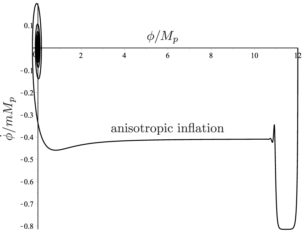
Adopting the inflaton potential
| (85) |
where is the inflaton mass, we have numerically studied the anisotropic inflationary model, and analyzed the evolution of the shear in detail. The gauge kinetic function is now
| (86) |
This inflationary model possesses the following two phases: (i) the conventional slow-roll inflationary phase and (ii) the anisotropic inflation after the contribution of the vector field becomes no longer negligible. If the initial energy density of the vector field is much smaller than that of the inflaton, the first phase is realized. During this phase, since the energy density of the vector field grows as , the vector field eventually comes to affect the dynamics of the inflaton field and the second anisotropic inflationary phase appears88 8 However, if there exist three or more U(1) fields with the same coupling function or the Yang-Mills field with the similar coupling to the inflaton field, an isotropic inflationary expansion becomes an attractor[33, 34].. We show one example in Fig. 6.
During the inflationary phase, we find that the effect of shear cannot become as large as the Hubble parameter. The measure of the anisotropy is described by , where and describe the average expansion rate and the magnitude of the spacetime shear, respectively. During the anisotropic inflation when the slow-roll approximation is valid, it is shown that the above anisotropic parameter satisfies [16]
| (87) |
where the slow-roll parameter in terms of the Hubble parameter is defined by
| (88) |
Eq. (87) means that is approximately the same as the slow-roll parameter , unless . Therefore, in spite of the strong coupling , the anisotropic parameter is much smaller than unity in the inflationary stage.

However, as shown in Fig. 7, the shear increases exponentially at the end of inflation.
In the evaluation of the generated baryon asymmetry in the text, we have used our numerical solution, but the increase of the shear at the end of inflation can be obtained (or restricted) by the semi-analytic approach, which we will show in the next section.
Appendix C Evaluation of the shear in anisotropic inflation
In this Appendix, we derive an upper limit of the spacetime shear at the end of the anisotropic inflation by the semi-analytic approach (See also [35]).
First we see the existence of the saturation of the shear magnitude from our numerical calculation. Using Eqs. (80) and (81), we describe the shear in terms of the slow-roll parameter as
| (89) |
Since the right hand side of Eq. (89) includes , its dependence on seems complicated. During the inflationary era satisfying , however, we find that increases monotonically as increases from the numerical calculation as shown in Fig. 8. The upper limit of the shear seems to exist and its value is evaluated at , which is
| (90) |
From Eq. (80), the anisotropy has the upper bound as
| (91) |
If we impose the weak energy condition on the effective matter field, must be larger than . As a result, the anisotropy must satisfy
| (92) |
This is the upper bound of the spatial anisotropy in Bianchi Type I Universe during the inflationary era.

We then evaluate the more precise upper bound of anisotropy by the semi-analytic approach. For a chaotic inflation with , and can be approximated by linear functions of the cosmic time during the second inflationary phase:
| (93) | ||||
| (94) |
where denotes the transition time from first isotropic inflationary phase to the second anisotropic inflationary phase. We have also used the approximation that the energy density of the vector field is given by the following constant
| (95) |
during anisotropic inflation [16]. Substituting these into the evolution equation of the shear given by Eq. (82), we find
| (96) |
with
| (97) |
where denotes the error function.
The anisotropic inflation takes place between and , where
| (98) |
is the end time of inflation evaluated by . Although the exponential function in Eq. (96) does not change so much during the above inflationary period, the amplitude grows rapidly and saturates around the end of inflation, just because of the typical behavior of the error function. As a result, we find that the shear increases drastically during the anisotropic inflationary phase.
We expect from the above saturation of that the anisotropy of the Universe becomes the largest at the end of the inflation. The maximal value is obtained at as
| (99) |
Here, we have used .
This result gives the better evaluation for the maximal value of anisotropy comparing with the previous result Eq. (87). The other approach to evaluate the maximal value by use of the higher-order expansion of the slow-roll parameter has been also given [35]. Our result is mostly the same as theirs.
Eq. (99) gives a good explanation for the tendency that the anisotropy of the Universe at the end of inflation is larger as the parameter increases as well as the fact that it is saturated for sufficiently large . Therefore, we do not expect an enormously large anisotropy at the end of the anisotropic inflation even with the very large .
References
- [1] A. H. Guth, Phy. Rev. D23, 347 (1981); D. Kananas, Astrophys. J. 241, L59 (1980); A. A. Starobinsky, Phys. Lett. B91, 99 (1980); K. Sato, Mon. Not. Roy. Astron. Soc. 195, 467 (1981).
- [2] P. A. R. Ade et al. [Planck Collaboration], arXiv: 1502.01589 [astro-ph.CO].
- [3] R. H. Cyburt, B. D. Fields, K. A. Olive and T. H. Yeh, arXiv: 1505.01076 [astro-ph.CO].
- [4] A. D. Sakharov, JETP Lett. 5, 24 (1967).
- [5] M. Yoshimura, Phys. Rev. Lett. 41, 281 (1978); S. Dimopoulos and L. Susskind, Phys. Rev. D18, 4500 (1978); S. Weinberg, Phys. Rev. Lett. 42, 850 (1979); M. Yoshimura, Phys. Lett. B88, 294 (1979).
- [6] V. A. Kuzmin, V. A. Rubakov and M. E. Shaposhnikov, Phys. Lett. B155, 36 (1985); M. E. Shaposhnikov, JETP Lett. 44, 465 (1986); M. E. Shaposhnikov, Nucl. Phys. B287, 757 (1987).
- [7] M. Fukugita and T. Yanagida, Phys. Lett. B174, 45 (1986).
- [8] I. Affleck and M. Dine, Nucl. Phys. B249, 361 (1985).
- [9] A. G. Cohen and D. B. Kaplan, Phys. Lett. B199, 251 (1987); A. G. Cohen and D. B. Kaplan, Nucl. Phys. B308, 913 (1988).
- [10] A. Dolgov, K. Freese, R. Rangarajan and M. Srednicki, Phys. Rev. D56, 6155 (1997).
- [11] J. March-Russell and M. McCullough, JCAP 1203, 019 (2012); K. Kamada and M. Yamaguchi, Phys. Rev. D85, 103530 (2012); F. Takahashi and M. Yamada, arXiv: 1510.07822 [hep-ph].
- [12] H. Davoudiasl, R. Kitano, G. D. Kribs, H. Murayama and P. J. Steinhardt, Phys. Rev. Lett. 93, 201301 (2004).
- [13] S. Weinberg, Phys. Rev. Lett. 48, 1303 (1982).
- [14] K. Kohri, T. Moroi and A. Yotsuyanagi, Phys. Rev. D73, 123511 (2006).
- [15] Kh. Saaidi and H. Hossienkhani, Astrophys. Space Sci. 333, 305 (2011); V. Fayaz and H. Hossienkhani, Astrophys. Space Sci. 344, 291 (2013).
- [16] M. Watanabe, S. Kanno and J. Soda, Phys. Rev. Lett. 102, 191302 (2009); J. Soda, Class. Quatum Grav., 29, 083001 (2012).
- [17] M. S. Turner and L. M. Widrow, Phys. Rev. D37, 2743 (1988); B. Ratra, Astrophys. J. 391 (1992).
- [18] S. Yokoyama and J. Soda, JCAP, 0808, 005 (2008).
- [19] R. M. Wald, Phys. Rev. D28, 2118 (1983).
- [20] G. W. Gibbons and S. W. Hawking, Phys. Rev. D15, 2738 (1977); S. W. Hawking and I. G. Moss, Phys. Lett. B110, 35 (1982); I. G. Moss and V. Sahni, Phys. Lett. B178, 159 (1986).
- [21] Y. Kitada and K. Maeda, Phys. Rev. D45, 1416 (1992); Y. Kitada and K. Maeda, Classical Quantum Gravity, 10, 703 (1993).
- [22] N. S. Manton, Phys. Rev. D28, 2019 (1983); F. R. Klinkhamer and N. S. Manton, Phys. Rev. D30, 2212 (1984); P. Arnold and L. McLerran, Phys. Rev. D36, 581 (1987).
- [23] E. W. Kolb and M. S. Turner, The Early Universe (Addison-Wesley, Redwood City, 1990).
- [24] J. Khoury, B. A. Ovrut, P. J. Steinhardt and N. Turok, Phys. Rev., D64, 123522 (2001).
- [25] P.J. Steinhardt and Neil Turok, Phys. Rev. D65, 126003 (2002).
- [26] P. J. E. Peebles and A. Vilenkin, Phys. Rev. D59, 063505 (1999).
- [27] K. Kajantie, M. Laine, K. Rummukainen and Y. Schroder, Phys. Rev. D67, 105008 (2003).
- [28] H. Li, M. Li and X. Zhang, Phys. Rev. D70, 047302 (2004); B. Feng, H. Li, M. Li and X. Zhang, Phys. Lett. B620, 27 (2005). M. C. Bento, R. G. Felipe and N. M. C. Santos, Phys. Rev. D71, 123517 (2005); G. Lambiase, Phys. Lett. B642, 9 (2006). G. Lambiase and G. Scarpetta, Phys. Rev. D74, 087504 (2006).
- [29] L. Ackerman, S. M. Carroll and M. B. Wise, Phys. Rev. D75, 083502 (2007).
- [30] M. Watanabe, S. Kanno and J. Soda, Prog. Theor. Phys. 123, 1041 (2010).
- [31] J. Kim and E. Komatsu, Phys. Rev. D88, 101301 (2013).
- [32] A. Naruko, E. Komatsu and M. Yamaguchi, JCAP 1504, 045 (2015).
- [33] K. Yamamoto, M. Watanabe and J. Soda, Class. Quantum Grav. 29, 145008 (2012).
- [34] K. Maeda and K. Yamamoto, Phys. Rev. D87, 023528 (2013); JCAP 12, 018 (2013).
- [35] J. Shi, X. Huang and T. Qiu, Sci. China Phys. Mech. Astron. 59, 4, 641001 (2016).