On the Polar Code Encoding in Fading Channels
Abstract
Besides the determined construction of polar codes in BEC channels, different construction techniques have been proposed for AWGN channels. The current state-of-the-art algorithm starts with a design-SNR (or an operating SNR) and then processing is carried out to approximate each individual bit channel. However, as found in this paper, for fading channels, an operating SNR can not be directly used in approximating the bit channels. To achieve a better BER performance, the input SNR for the polar code construction in fadding channels is derived. A selection of the design-SNR for both the AWGN and the fading channels from an information theoretical point of view is studied. Also presented in this paper is the study of sacrificing a small data rate to gain orders of magnitude increase in the BER performance.
I Introduction
Polar codes have been proposed by Erdal Arkan in [1]. The fact is that polar codes can achieve the channel capacity at a low encoding and decoding complexity of . The original format of polar codes in [1] is non-systematic. Later, a systematic version of polar codes was invented by Arkan in [2], which is shown to outperform the non-systematic polar codes in terms of the BER performance.
Channel combining and splitting realize the polarization of channels. After these two stages, channels are polarized in the sense that bits transmitting in these channels either experience almost noiseless channels or almost completely noisy channels for a large . Then one can easily achieve a rate of transmission close to the channel capacity, simply by choosing to transmit over the good bit channels and fix the bits in bad channels. However, at a finite block length and a data rate ( being the number of information bits in each codeword of length ). A ranking algorithm of the bit channels according to their bit error rate (BER) becomes necessary to select good channels out of the channels. This selection of bit channels completely defines a polar code for any given underlying channel.
In this paper, we consider the underlying channels to be AWGN channels and fading channels. To select the good indices in a AWGN channel, as stated in [1], a Monte-Carlo simulation can be used to sort the bit channels. This algorithm has a high complexity of , where is the number of iterations of the Monte-Carlo simulation. A more recent construction algorithm for AWGN channels is proposed by Tal and Vardy [3] which is based on an earlier proposal from Mori and Tanaka [4] [5]. The algorithm in [3] is by far the best construction algorithm with a complexity of where is a user defined variable (Note that this complexity excludes the quantization of a AWGN channel to a discrete-alphabet channel). In [6], the estimation of bit-channels based on a Gaussian approximation is proposed. This was found to well-approximate the actual bit-channels of polar codes in [7] and [8]. A similar algorithm after the original proposal in [6] was studied in [7], [8]. The Gaussian approximation algorithm involves relatively higher complexity function computations, with a complexity of function computations (excluding the selection of K best among N metrics obtained).
From the discussions of the constructions of [1, 3, 6, 7, 8] for AWGN channels, it’s seen that all algorithms start with a specified value of the signal-to-noise ratio (SNR). In practice, it’s difficult (or expensive) to compute the code indices with the variation of the SNR. Hence, a design-SNR is desired to construct polar codes that produce a good BER performance for a given data rate and possible variations of the system SNR. In [9], a design-SNR is produced from extensive simulations.
In this paper, we propose a selection of the design-SNR for any data rate from an information theoretical analysis. For a system with an operating SNR and a data rate , a design-SNR can be used to obtain the code indices instead of the operating SNR. Both AWGN channels and block fading channels are considered in the analysis of this paper. In block fading channels, we also conduct a study of sacrificing a small data rate in the large-SNR region to gain orders of magnitude increase of the BER performance. Simulation results are provided to verify the validness of the selection of the design-SNR and the great increase of the BER performance at a small cost of the data rate.
The rest of the paper is organized as follows. In Section II, we describe fundamentals of non-systematic polar code and systematic polar code. Section III introduces a transmission scheme which can improve the BER performance in orders of magnitude at a small cost to the data rate in fading channels. In Section IV, we analyze the design-SNR and present a selection of the design-SNR for both the AWGN and the fading channels. We finally present our simulation results in Section V and conclude this paper in Section VI.
II Polar Code Fundamentals
In this section, the relevant theories about non-systematic polar codes and systematic polar codes are presented.
II-A Non-Systematic Polar Codes
A polar code may be specified completely by , where is the length of a codeword, is the number of information bits encoded per codeword, is a set of indices called information bit locations from , and consists of the frozen bits. For an polar code, a codeword is obtained as:
| (1) |
where denotes the submatrix of formed by the rows with indices in , and equals for any . Here is the standard polarizing kernel .
The Successive Cancellation Decoding (SCD) algorithm in [1] uses a decoding operation that is similar to the belief propagation (BP) algorithm. The likelihoods evolve in the inverse direction from the right to the left, as illustrated with an example in [1], using a pair of likelihood transformation equations. Then the bit decisions are made at the left of the circuit and is used in the rest of the decisions.
II-B Systematic Polar Codes
The systematic polar code split the codeword into two parts by writing . So (1) can be written as
| (2) |
| (3) |
where the and , the matrix is a submatrix of the generator matrix with elements , and similarly for the other submatrices. The proposition in [2] says that if (and only if) and have the same number of elements and is invertible, there exists a systematic encoder . It performs the mapping . The vector can be obtained by computing
| (4) |
In [2], we’ve known that is the necessary conditions of establishing the one-to-one mapping . In the rest of the paper, the systematic encoding of poalr codes will use , instead of . So, the mapping of (2) and (3) can be rewritten as:
| (5) |
| (6) |
III Polar Codes Transmission over
Fading Channels
In this section, we present a transmission scheme which can improve the BER performance in orders of magnitude at a small cost to the data rate.
The underlying channel we consider is
| (7) |
where follows a normal distribution , is the additive white Gaussian noise with mean 0 and variance , and is the binary modulated transmitted symbol: . The encoded bits is thus modulated to . The channels experienced by , denoted as , are assumed to be i.i.d and are stable for code blocks. This is a block fading channel model which can be observed in various wireless communication scenarios. In our study, assume is known at the receiver. With the channel estimation of , the underlying channel in (7) can be converted to:
| (8) |
Due to the limitations of the channel estimation algorithms, there is a limit of the channel values below which the estimation is unreliable. In this paper, we do not attempt to discuss the limitations of various channel estimation algorithms. Instead, we keep this limit of channel values as a variable . As seen in the sequel, the change of with channel estimation algorithms does not increase the complexity of our algorithm.
For a given , a percentage can be calculated: , which translates to the fact that observations at the receiver are not reliable. These unreliable observations in return will cause a poor BER performance. In this case, to maintain a given BER performance, either a higher SNR or a lower data rate can be applied. Here a question arises: whether the SNR should be increased or the data rate should be lowered? Which selection yields a better performance? To answer this question, we resort to the work of [10] for the asymptotic behavior of polar codes. The relationship of the block error rate with the data rate and the capacity of the underlying channel is rewritten as below from [10]
| (9) |
where is the reverse function of . The fundamental information theoretical analysis yields the channel capacity of (7) as
| (10) |
where is the SNR and is defined as
| (11) |
As the evaluation of (11) is not closed, we can use an upper bound of to approximate . The function is concave in terms of the data rate when fixing . It’s also concave in terms of = for a fixed data rate . Fig. 1 shows as a function of the data rate under several SNR values.

From Fig. 1, we can see clearly that with a fixed data rate, increasing SNR does not yield a significant BER performance increase at high SNR regions. Instead, decreasing the data rate is a better choice. With this principle, we propose the following Algorithm 1 to improve the BER performance in fading channels whenever a certain amount of bad channels are detected. In this algorithm, is a channel index matrix chosen according to the quality of bit channels and is approximately equal to .
With Algorithm 1, a system in a fading channel first selects a according to the channel estimation algorithm. Then another value is selected which can be a tradeoff between the BER performance and the data rate decrease. When (or any number smaller than ) unreliable channel estimations are detected, a data rate decrease is performed: channels are changed from the data-bearing channels to the frozen channels. Here is the calculated channel capacity according to the operating SNR and the capacity of in (11). This decrease of is that the unreliable observations theoretically lose information bits.
It’s worthwhile to emphasize that the variation of and does not increase the complexity of Algorithm 1. This resides in the choice of the sorted channels . A change of and only changes the number which eventually only results in how many entries are selected from . As long as is provided, the complexity does not change with the variation of the parameter and . In the next Section, we provide a theoretical way to construct for a given data rate .
IV Design-SNR Analysis
For a system with an operating SNR = and a data rate in AWGN channels, a construction based on [3] can be carried out with this . Theoretically, with any change in SNR, a new construction should be obtained to accommodate this change of SNR. However, to a lot of systems, a real time construction is too complicated to perform. In [9], a design-SNR is found from simulations which can produce a good BER performance for a range of SNRs. In this paper, we provide an information theoretical foundation for the existence of the design-SNR for a fixed data rate .
Let’s first look at the AWGN channels. The constellation constrained channel capacity of the AWGN channel is shown in (10) with . For a fixed data rate , the required SNR to achieve this data rate can be obtained as:
| (12) |
where is the inverse function of in (11). Let’s denote the required SNR for a data rate as . For a fixed data rate , this is the design-SNR which should be used for the construction of polar codes.
For fading channels, in order to use the construction algorithm like [3], we need to convert the channel in (8) to an AWGN channel. One way to do this is to take the mean of the channel in (8) with respect to
| (13) |
which has an equivalent of
| (14) |
In (14), . For the normal distribution , . Therefore, we have
| (15) |
If a point-by-point construction is to be carried out for the underlying channel in (7), then the input SNR for the construction algorithm should be a modified version shown in (15) instead of directly using the operating SNR . This point is verified in the simulation results in the next section: the BER performance of polar codes constructed using is poorer than that constructed by .
Like AWGN channels, a design-SNR also exists for fading channels. However, from the simulation results, we find that the design-SNR does not follow the relationship shown in (15): a design-SNR of for a AWGN channel does not produce a design-SNR (all in dB) for the fading channel in (7). Surprisingly, AWGN channels and the fading channels in (7) share the same design-SNR. Simulation results are provided to show the performance of the design-SNR selections for AWGN channels and fading channels.
V Numerical Results
To verify the fading channel transmission scheme of polar codes in Algorithm 1 and the design-SNR selection, simulation results are provided in this section. All the polar codes construction in this section are based on [3].
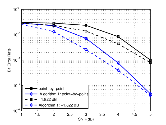
Algorithm 1 is carried out using the following parameters: , , , and . The sorted channel indices are generated in two ways: 1) point-by-point construction of (15); 2) the design-SNR for the data rate . The design-SNR is computed using (12). For , the desgin-SNR is computed to be dB. The BER performance of systematic polar codes are shown in Fig. 2, where the solid squared line is the original BER performance with code indices selected from the point-by-point construction with the input SNR given in (15) and the solid line with diamonds is the BER performance of polar codes constructed this way with Algorithm 1 running at the same time. Clearly, the BER performance is greatly improved with Algorithm 1: the BER is reduced by 21 times while the data rate is only reduced by 15%. The two dashed lines in Fig. 2 are the corresponding BER performance using the design-SNR -1.822 dB instead of a point-by-point construction. The same improvement is observed when running our Algorithm 1.
Fig. 3 shows the BER performance comparison between the construction using the design-SNR and the point-by-point construction in AWGN channels. The polar code has a block length and . The design-SNR for this case is the same as in Fig. 2. The two solid lines in Fig. 3 are the non-systematic BER performance using the point-by-point construction and the design-SNR construction. From Fig. 3, it can be seen that the BER performance of non-systematic polar codes using the design-SNR construction matches closely with the point-by-point construction. The same can be seen for the systematic polar codes.
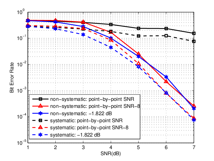
The simulation results of the design-SNR in fading channels are shown in Fig. 4. The polar code block length is again and the data rate is . According to Section IV, in fading channels, the design-SNR is the same as that of the AWGN channels. Therefore in this case, the design-SNR is -1.822 dB. The two square lines (solid and dashed) are the BER performance of non-systematic and systematic polar codes constructed point-by-point using the operating SNR. The two lines (solid and dashed) with up-triangles are the BER performance of non-systematic and systematic polar codes constructed point-by-point using the operating SNR - 8 as shown in (15). And the two lines (solid and dashed) with hexagrams are the BER performance of non-systematic and systematic polar codes constructed using the design-SNR dB. The first thing to notice from Fig. 4 is that the BER performance of both the systematic and non-systematic polar codes with the point-by-point construction using the operating SNR is much worse than the construction using SNR - 8 and the design-SNR of -1.822 dB. This shows that the point-by-point construction of polar codes in fading channels of (7) should use an input SNR in (15) instead of directly using the operating SNR. In the mean time, the BER performance of both the systematic and non-systematic polar codes with the design-SNR is either better or equal to that of the point-by-point construction using SNR - 8 dB. The design-SNR clearly can be used for the polar code construction in fading channels.

VI Conclusion
In this paper, we propose a fading channel transmission scheme of polar codes which can greatly improve the BER performance at a small cost to the data rate. An algorithm is given to implement the proposed scheme. In the mean time, a design-SNR selection is proposed based on an information theoretical analysis. This design-SNR selection is valid for both the AWGN channels and fading channels. Simulation results are provided which verified the transmission scheme and the design-SNR selection.
References
- [1] E. Arikan, “Channel Polarization: A Method for Constructing Capacity-Achieving Codes for Symmetric Binary-Input Memoryless Channels,” IEEE Transactions on Information Theory, vol. 55, no. 7, pp. 3051–3073, 2009.
- [2] ——, “Systematic Polar Coding,” IEEE Communications Letters, vol. 15, no. 8, pp. 860–862, August 2011.
- [3] I. Tal and A. Vardy, “How to construct polar codes,” Information Theory, IEEE Transactions on, vol. 59, no. 10, pp. 6562–6582, Oct 2013.
- [4] R. Mori and T. Tanaka, “Performance of polar codes with the construction using density evolution,” IEEE Communications Letters, vol. 13, no. 7, pp. 519–521, Jul. 2009.
- [5] ——, “Performance and Construction of Polar codes on Symmetric Binary-Input Memoryless Channels,” in IEEE International Symposium on Information Theory, June 2009, pp. 1496–1500.
- [6] P. Trifonov, “Efficient Design and Decoding of Polar Codes,” IEEE Transactions on Communications, vol. 60, no. 11, pp. 3221–3227, November 2012.
- [7] H. Li and J. Yuan, “A practical construction method for polar codes in AWGN channels,” in TENCON Spring Conference, 2013 IEEE, Apr. 2013, pp. 223–226.
- [8] D. Wu, Y. Li, and Y. Sun, “Construction and block error rate analysis of polar codes over AWGN channel based on Gaussian approximation,” IEEE Communications Letters, vol. 18, no. 7, pp. 1099–1102, Jul. 2014.
- [9] H. Vangala, E. Viterbo, and Y. Hong, “A comparative study of polar code constructions for the awgn channel,” arXiv preprint arXiv:1501.02473, 2015.
- [10] S. Hassani, R. Mori, T. Tanaka, and R. Urbanke, “Rate-Dependent Analysis of the Asymptotic Behavior of Channel Polarization,” Information Theory, IEEE Transactions on, vol. 59, no. 4, pp. 2267–2276, 2013.