A Desired PAR-Achieving Precoder Design for Multi-User MIMO OFDM based on
Concentration of Measure

Multiple-input multiple-output (MIMO) and orthogonal frequency division multiplexing (OFDM) have been regarded as key technologies for wireless communication systems to boost the network capacity. Regretfully, the OFDM has a fundamental drawback of high peak-to-average power ratio (PAR) [3] that can be further aggravated by MIMO precoding techniques [4], and it may ultimately result in the use of linear power amplifiers in spite of their high cost [5].

Under this practical challenge, the authors of [6] and [7] effectively used redundant spatial dimensions to considerably reduce the PAR, while providing the inherent MIMO precoding gain for the multi-user (MU) multiple-input single-output and the single-user MIMO, respectively.

In this paper, we propose a MU-MIMO precoding scheme for OFDM system that can achieve a desired PAR performance at the minimum cost by utilizing the redundant spatial dimensions. The cost is defined as the received SNR degradations, compared to those of SNRs that would have been obtained by the original block diagonalization (BD) scheme [8, 9].

For this purpose, we modify the BD precoding matrix with the introduction of design parameters for the beamforming and cost control, and formulate their relation as a quadratic over linear expression motivated by an ellipsoid constraint in [7]. By taking advantage of the concentration of measure [1, 2], meaning that most of the volume of a high dimensional convex body are concentrated near its boundary, we clarify that the average power consumption hardly changes with respect to the design parameters. Then it offers an opportunity for an accurate approximation of the PAR measure, which is reflected in a convex constraint to guarantee the desired PAR.

The volume concentration phenomenon is intensified as the number of subcarriers $(K)$ increases, which makes the approximated PAR more accurate. As a consequence, the proposed scheme almost exactly achieves the desired PAR on average, and asymptotically attains the desired PAR at the $10^{-3}$ point of its complementary cumulative distribution function (CCDF), as $K$ increases.¹¹ 1 Throughout this paper, $\mathbb{N},\mathbb{R},\mathbb{R}_{+}$ and $\mathbb{C}$ denote the sets of natural numbers, real numbers, positive real numbers and complex numbers, respectively. For $n\in\mathbb{N}$, denote $[1:n]=\{1,...,n-1,n\}$. For a set of matrices $\{{\mathbf{A}}_{k}\}$, ${\sf blkdiag}(\mathbf{A}_{1},...,\mathbf{A}_{n})$ and ${\cal N}(\mathbf{A}_{k})$ respectively denote the block diagonal matrix composed of $\{\mathbf{A}_{k}\}$ and a set of basis vectors on the null space of $\mathbf{A}_{k}$ except for zero vector.

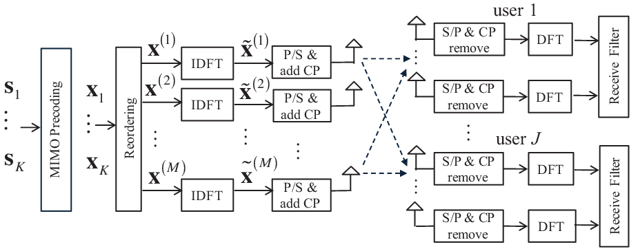
In this section, we state the system model and the related studies. Consider the MU-MIMO OFDM system depicted in Fig. 1, where a transmitter and each user are equipped with $M$ and $N$ antennas respectively, where $(J-1)N<M$ for $J\geq 2$ and $N\leq M$ for $J=1$. The transmitter wishes to send a signal vector ${\mathbf{s}}_{k}^{[j]}\in\mathbb{C}^{d_{j}}$ to the $j^{th}$ user through the $k^{th}$ subcarrier for $j\in[1:J]$ and $k\in[1:K]$, where ${\mathbf{s}}_{k}^{[j]}$ consists of $d_{j}$ data streams drawn from a discrete constellation set ${\cal A}$, and $d_{\Sigma}=\sum\nolimits_{j=1}^{J}{{d_{j}}}\leq M$.

Let ${\mathbf{H}}_{k}^{[j]}\in\mathbb{C}^{N\times M}$, ${\bf{F}}_{k}^{[j]}\in{\mathbb{C}^{{M}\times d_{j}}}$, ${\bf{R}}_{k}^{[j]}\in{\mathbb{C}}^{d_{j}\times N}$ and ${\mathbf{w}}_{k}^{[j]}\in{\mathbb{C}^{{N}}}$ respectively denote the channel matrix composed of i.i.d. complex coefficients, the precoding matrix, the receiving filter and the additive noise that follows circularly symmetric complex Gaussian ${\cal{C}}{\cal{N}}(\mathbf{0},\sigma^{2}\mathbf{I})$ for all $j\in[1:J]$ and $k\in[1:K]$. We assume that the transmitter completely knows $\{{\mathbf{H}}_{k}^{[j]}\}_{k\in[1:K],j\in[1:J]}$. Then the received signal vector of the $j^{th}$ user, denoted by ${\mathbf{y}}_{k}^{[j]}\in\mathbb{C}^{d_{j}}$, is given by

for all $k\in[1:K]$ and $j\in[1:J]$.

Let us denote ${{\mathbf{s}}_{k}}={[{{\mathbf{s}}_{k}^{[1],T},\ldots,{\mathbf{s}}_{k}^{[J],T}}]}^{T}\in\mathbb{C}^{d_{\Sigma}\times 1}$, ${{\mathbf{F}}_{k}}=[{{\mathbf{F}}_{k}^{[1]},\ldots,{\mathbf{F}}_{k}^{[J]}}]\in\mathbb{C}^{M\times d_{\Sigma}}$ and ${\bf{x}}_{k}=\mathbf{F}_{k}\mathbf{s}_{k}$ where ${\sf E}[{{{\mathbf{s}}_{k}}{\mathbf{s}}_{k}^{H}}]=\frac{{{{\cal P}_{s}}}}{{{d_{\Sigma}}}}{{\mathbf{I}}_{{d_{\Sigma}}}}$ for all $k\in[1:K]$, and define $\mathbf{s}={[{{\mathbf{s}}_{1}^{T},\ldots,{\mathbf{s}}_{{K}}^{T}}]}^{T}\in\mathbb{C}^{Kd_{\Sigma}}$, ${\mathbf{F}}={\sf blkdiag}({{{\mathbf{F}}_{1}},\ldots,{{\mathbf{F}}_{{K}}}})\in\mathbb{C}^{MK\times Kd_{\Sigma}}$ and $\mathbf{x}={[{{\mathbf{x}}_{1}^{T},\ldots,{\mathbf{x}}_{{K}}^{T}}]}^{T}\in\mathbb{C}^{MK\times 1}$, where ${\sf E}[{{{\mathbf{s}}}{\mathbf{s}}^{H}}]=\frac{{{{\cal P}_{s}}}}{{{d_{\Sigma}}}}{{\mathbf{I}}_{{Kd_{\Sigma}}}}$ and ${\sf E}[{\left\|{{\mathbf{x}}}\right\|^{2}}]\leq K{{\cal{P}}_{s}}$. All elements in $\mathbf{x}$ are distributed to the $M$ transmission antennas through an one-to-one mapping matrix $\mathbf{\Phi}\in\mathbb{R}^{MK\times MK}$ in the reordering block of Fig. 1. This process is also given by [6] and is represented as

where $\mathbf{x}^{(i)}$ is the signal vector transmitted by the $i^{th}$ antenna, and $\mathbf{\Phi}$ is one of the permutation matrices, where their rows are composed of standard basis vectors of $\mathbb{R}^{1\times MK}$.

Let ${{{\tilde{\mathbf{x}}}}}^{(i)}={{\mathbf{Q}}_{i}}{{\mathbf{x}}}^{(i)}$ be time-domain signals transmitted by the $i^{th}$ antenna, where ${{\mathbf{Q}}_{i}}$ is the $K$-point inverse discrete Fourier transform (IDFT) matrix. We define ${\mathbf{Q}}={\sf blkdiag}({{\mathbf{Q}}_{1}},\ldots,{{\mathbf{Q}}_{M}})$, and assume that the channel tap length is always shorter than the cyclic prefix length.

Then the PAR of the $i^{th}$ transmission antenna is defined as

for all $i\in[1:M]$. Even if $\mathbf{\Phi}$ can be regarded as a design parameter, we consider a simplified model by assuming $\mathbf{\Phi}=\mathbf{I}$ similar to [6]. Let us define a relaxed PAR measure in terms of a single linear system with regard to $\mathbf{x}\in\mathbb{C}^{MK}$ as

where $\tilde{\mathbf{x}}={\mathbf{Qx}}$, and (4) is also given by [6, 7].

As a preliminary to this paper, we briefly introduce the BD precoding scheme in the following remark [8, 9].

In [5], the $l_{\infty}$-norm minimization technique is introduced as an alternative way to reduce the PAR due to non-convexity of the PAR measure. It is actively used to develop MIMO precoding schemes, such as [6] for $N=1$ and $J<M$ and [7] for $J=1$ and $N<M$. In this work, our main focus is not the PAR reduction by $l_{\infty}$-norm minimization, but the achivement of the desired PAR performance at the minimum cost for an arbitrary $J$, $M$ and $N$ where $(J-1)N<M$, and also discuss the impact of a large $M$ and $K$.

In this section, we specifically describe the proposed MIMO precoding scheme and discuss its related issues.

In this section, we numerically evaluate the performance of the proposed scheme assuming $N=J=2$ and $d_{1}=d_{2}=1$, and $M$ and $\zeta$ are given in Table I, and the channel coefficients and the data streams are respectively drawn from i.i.d. ${\cal CN}(0,1)$ and 16-QAM constellation set $\left(|{\cal A}|=16\right)$. Through large enough realizations of them, we aggregate $\hat{\mathbf{t}}$ and $\gamma$ from $({\cal C})$. The CCDF is defined as ${\sf{Pr}}[\text{PAR}^{(i)}\geq{\text{PAR}}_{0}]$.

Fig. 2 plots CDFs of $\hat{\gamma}$ with respect to various $M$ and $\zeta$, and their corresponding empirical mean of $\text{PAR}^{(i)}$ samples is represented in Table I, which shows the effectiveness of the proposed scheme in terms of the average PAR performance. The CDFs of $\hat{\gamma}$ for $\zeta=1.5$ show that the more redundant spatial dimensions do not always guarantee the better performance, which can be inferred from Proposition 2. Thus, $d_{\Sigma}$ or $K$ needs to be increased with an increase of $M$ to avoid the substantial reduction of the feasible space, especially for quite a challenging constraint such as $\zeta=1.5$.

Fig. 3 plots the CDFs of $\hat{\gamma}$, CCDFs of $\text{PAR}^{(i)}$ and CDFs of $\text{PAR}^{(i)}$ from left to right with respect to various $K$ when $M=4$ and $\zeta=1.8$. In this figure, the variance of both $\text{PAR}^{(i)}$ and $\hat{\gamma}$ decreases as $K$ increases, so that the samples of $\text{PAR}^{(i)}$ and $\hat{\gamma}$ are increasingly concentrated near their empirical mean value. Thus, the proposed scheme can asymptotically attain $10\log_{10}(\zeta)$ [dB] at $\text{CCDF}=10^{-3}$ as $K$ increases. This result can be inferred from the first discussion item in Section III-C. In Fig. 3, the $\text{PAR}^{(i)}$ samples are concentrated near 2.79 [dB] as $K$ grows, thus the proposed scheme can asymptotically attain $\text{PAR}_{0}=2.79$ [dB] at $\text{CCDF}=10^{-3}$ as $K$ grows. These imply that the variance of $\hat{\gamma}$ and $\text{PAR}^{(i)}$ when $M=16$ and $\zeta=1.5$ would be reduced if $K$ increases.

The bit error rate (BER) performance degradation compared to the original BD described in Remark 1 $(\gamma=1)$ can be readily explained, since the received SNR difference of two schemes is expressed as $10\log_{10}(\hat{\gamma})$ [dB]. It means that a BER performance curve of the proposed scheme is not shifted more than $10\log_{10}(\hat{\gamma})$ [dB] compared to that of Remark 1. If $K=64,M=4$ and $\zeta=1.8$, then $\hat{\gamma}\geq 0.8$ as plotted in Fig. 3, thus the BER performance degradation is not greater than $10\log_{10}(0.8)\approx 0.97$ [dB]. Also, this 0.97 [dB] gets further reduced as $K$ increases, since the minimum value of the $\hat{\gamma}$ samples increases up to their empirical mean value.

When $\hat{\gamma}$ is not close to 1, the approximation of $\sqrt{\hat{\gamma}}$ in our analysis would be inaccurate and lead to larger degradation of the BER performance, so that $\hat{\gamma}$ of around 1 is of our interest.

We proposed a MIMO precoding scheme that can achieve the desired PAR. Numerical results show that it can achieve not only the desired PAR on average, but also attains the desired PAR at the $\text{CCDF}=10^{-3}$ if $K$ is arbitrarily large. Also, for the application in a large-scale MIMO system, $\zeta$ and $d_{\Sigma}$ need to be carefully chosen considering the feasible space size.

References

- [1] M. Ledoux, The concentration of measure phenomenon. Providence, R.I. : American Mathematical Society, 2001.
- [2] D. L. Donoho, “High-dimensional data analysis: The curses and blessings of dimensionality,” in Proc. AMS Conference on Math Challenges of the 21st Century, 2000.
- [3] E. Larsson, O. Edfors, F. Tufvesson, and T. Marzetta, “Massive MIMO for next generation wireless systems,” IEEE Commun. Mag., vol. 52, no. 2, pp. 186–195, Feb. 2014.
- [4] H.-J. Su, C.-P. Lee, W.-S. Liao, R.-J. Chen, C.-L. Ho, C.-L. Tsai, and Z. Yan-Xiu, “Peak-to-average power ratio issue of beamforming/precoding schemes,” in IEEE C802.16m-08/1302, Oct. 2008.
- [5] A. Aggarwal and T. H. Meng, “Minimizing the peak-to-average power ratio of OFDM signals using convex optimization,” IEEE Trans. Signal Process., vol. 54, no. 8, pp. 3099–3110, Aug. 2006.
- [6] C. Studer and E. G. Larsson, “PAR-aware large-scale multi-user MIMO-OFDM downlink,” IEEE J. Sel. Areas Commun., vol. 31, no. 2, pp. 303–313, Feb. 2013.
- [7] H.-S. Cha, H. Chae, K. Kim, J. Jang, J. Yang, and D. K. Kim, “Generalized inverse aided PAPR-aware linear precoder design for MIMO-OFDM system,” IEEE Commun. Lett., vol. 18, no. 8, pp. 1363–1366, Aug. 2014.
- [8] R. Chen, Z. Shen, J. Andrews, and R. Heath, “Multimode transmission for multiuser MIMO systems with block diagonalization,” IEEE Trans. Signal Process., vol. 56, no. 7, pp. 3294–3302, Jul 2008.
- [9] C.-B. Chae, S. Shim, and R. Heath, “Block diagonalized vector perturbation for multiuser MIMO systems,” IEEE Trans. Wireless Commun., vol. 7, no. 11, pp. 4051–4057, Nov. 2008.
- [10] J. Hopcroft and R. Kannan, “Foundations of data science,” Available online only: http://research.microsoft.com/en-us/people/kannan/book-dec-30-2013.pdf, Dec. 2013.
- [11] A. Barg and D. Nogin, “Bounds on packings of spheres in the Grassmann manifold,” IEEE Trans. Inf. Theory, vol. 48, no. 9, pp. 2450–2454, Sep. 2002.
- [12] T. Tao, Topics in random matrix theory. American Mathematical Society Providence, RI, 2012.
- [13] I. L. Dryden, “Statistical analysis on high-dimensional spheres and shape spaces,” Ann. Statist., vol. 33, no. 4, pp. 1643–1665, Aug. 2005.
- [14] H. H. Bauschke and P. L. Combettes, Convex Analysis and Monotone Operator Theory in Hilbert Spaces. Springer, 2011.
- [15] S. Boyd and L. Vandenberghe, Convex Optimization. Cambridge University Press, 2004.
- [16] O. Henkel, “Sphere-packing bounds in the Grassmann and Stiefel manifolds,” IEEE Trans. Inf. Theory, vol. 51, no. 10, pp. 3445–3456, Oct. 2005.