Markov Switching asymmetric GARCH Model: Stability and Forecasting
Abstract
A new Markov switching asymmetric GARCH model is proposed where each state follows a logistic smooth transition structure between effects of positive and negative shocks. This consideration provides better forecasts in many financial time series. The asymptotic finiteness of the second moment is investigated. The parameters of the model are estimated by applying MCMC methods through Gibbs and griddy Gibbs sampling. Applying the log return of some part of SP 500 indices, we show the competing performance of in sample fit and out of sample forecast volatility and value at risk of the proposed model. The Diebol-Mariano test shows that the presented model outperforms all competing models in forecast volatility.
Keywords: Markov switching, Leverage effect, Smooth transition, DIC, Bayesian inference, Griddy Gibbs sampling.
Mathematics Subject Classification: 60J10, 62M10, 62F15.
1 Introduction
Volatility modeling in financial time series has been widely studied over past few decades. The ARCH and
GARCH models , introduced by Engle [17] and Bollerslev [11], are surely the most popular classes of volatility models. Hamilton and Susmel [26] introduced the Markov-Switching GARCH (MS-GARCH) by merging GARCH model with a hidden Markov chain, where each state allows a different GARCH behavior. Such structure improves forecasting of volatilities. Gray [22], Klaassen [29] and Haas, et al. [24] proposed some different variants of MS-GARCH models. For further studies on MS-GARCH models, see Abramson and Cohen [1], Ardia [5], Alemohammad et. al [2] and Bauwens et al. [8].
One restriction of the GARCH model is its symmetry to the sign of past shocks. This is improved by letting the conditional variance to be a function of size and sign of the preceding observation. Such studies started by Black [10], who investigated asymmetric effects of positive and negative shocks on volatilities. This consideration is important in financial markets as there exists higher volatility in response to bad news (negative shocks). [21]. Study of the asymmetric GARCH started by Engle [18] and continued as the Exponential GARCH (EGARCH) model by Nelson [35], GJR-GARCH model by Glosten, et al.[20] and Threshold GARCH (TGARCH) model by Zakoian [40]. The other asymmetric structures are Smooth transition models introduced by Gonzalez-Rivera [21], Ardia [5], Medeiros and Veiga [33], and Haas et al. [25].
In this paper, we study some Markov switching GARCH model where the volatility in each regime is coupled with the smooth transition between the effects of negative and positive schocks. More precisely, the presented model considers different smooth transition structure by states where each state describes some time dependent convex combination between asymmetric effects of positive and negative and shocks. The new model obviates the absence of asymmetric property in the Markov switching GARCH model and switching between different levels of volatility in the Smooth transition GARCH model (ST-GARCH), presented by Lubrano [32].
Ardia [5] considered some MS-GARCH model where the asymmetric effects of volatilities are considered by applying
indicator functions of some predefined non-positive thresholds in states. This cause a sudden shift of volatility structure at corresponding threshold in each state.
Alemohammad et. al [2] considered a Markov switching GARCH model where the smooth transition between structures for high and low volatilities are in effect of size of the preceding return.
In this paper we study the case where the volatility structure in each state follows some smooth transition between the effects
of positive and negative shocks based on the
preceding log return. So it is expected to provide much better fitting, especially
when smooth transitions between such effects are evident.
As such model employs all past observations, we reduce the volume of calculations by proposing a dynamic programming algorithm. We also derive sufficient condition for stability of the model by applying
the method of Abramson and Cohen [1] and Medeiros [33].
Markov chain Monte Carlo (MCMC) methods are widely applied for parameter estimation of the regime switching GARCH models, see, e.g, [8] and [5]. As nonlinearity is considered, the likelihood function becomes tricky to maximize since it is hard to differentiate, see [32]. In addition the existence of latent variables
also makes the Bayesian method to be required. The privileges of the MCMC methods is that avoid the common problem of local maxima encountered in the Maximum likelihood (ML) estimation, see [4] (section 7.7).
The parameters of our model are estimated by applying MCMC methods through Gibbs and Griddy-Gibbs sampling.
We present a simulation example to show the competitive performance of our model in compare to GARCH, MS-GARCH and ST-GARCH models. Using 500 indices from to we show that our model has much better fitting by providing less forecasting error, better performance base on Diebold-Mariano test and value at risk of out-of-sample forecasting of one day ahead volatility,
in compare with GARCH, MS-GARCH, EGARCH,GJR-GARCH and ST-GARCH models.
We also show that our model outperforms the competing models for in-sample fit by using the Deviance information criterion.
The Markov switching smooth transition GARCH model is presented in section 2. Section 3 is devoted to the statistical properties of the model. Estimation of the parameters of the model are studied in section 4. Simulation studies are followed to show competing performance of presented model in section 5. Section 6 is dedicated to the analysis of the efficiency of the proposed model by applying the model to the SP 500 indices for to . Section 7 concludes.
2 Markov switching asymmetric GARCH model
We consider the Markov switching smooth transition GARCH model, in summary MS-STGARCH as
| (2.1) |
where are iid standard normal variables, is an irreducible and aperiodic Markov chain on finite state space with transition probability matrix where , and stationary probability measure Also given that , (the conditional variance of regime j) is defined as
| (2.2) |
where
| (2.3) |
and the weights () are logistic function of the past observation as
| (2.4) |
which are monotonically increasing with respect to previous observation and are bounded , . The parameter is called the slope parameter. The weight function goes to one when and so tends to . Also it goes to zero when and so tends to . Therefore the effect of negative shocks are mainly described by and of positive shocks by . As often negative shocks have greater effect on volatilities than positive ones, one could assume that in each regime. To impose the idea in model building, we recommend to consider a higher prior for in each state and any estimation procedure. Logistic weight functions in states have the potential to describe different speed for smooth transitions which are in effect of and also different effect limits as and . This enables one to provide a flexible model for describing such different transitions. Plots of such logistic weight functions for the returns of SP 500 indices, which are studied later in this paper, are presented in Figure 1. Indeed in each regime the coefficient of is time dependent that causes the volatility structure being under the influence size and sign of the observations and it makes distinct from GARCH model.
As , the logistic weight function considers a step function for positive and negative shocks. When approaches to zero, goes to and the MS-STGARCH model tends to the Markov switching GARCH model(MS-GARCH). In the case of single regime, our model is the smooth transition GARCH (STGARCH) model that is introduced by Lubrano [32].
It is assumed that and are independent. Sufficient conditions to guarantee strictly positive conditional variance (2.2) are that to be positive and being nonnegative.

3 Statistical Properties of the model
In this section, the statistical properties of the MS-STGARCH model are investigated and the conditional density and variance of the process is obtained. As the evaluation of the asymptotic behavior of the second moment in our model isn’t so easy to follow, we apply the method of Abramson and Cohen [1] and Medeiros [33] to obtain an appropriate upper bound for the asymptotic value of the unconditional variance to show its stability.
3.1 Conditional density and variance
Let be the information up to time t. Following the method of Alemohammad et al. [2], the conditional density function of given past information can be written as
| (3.5) |
where is the probability density function of the standard normal distribution and , that is obtained in the following remark.
Remark 3.1
The value of is obtained recursively by
| (3.6) |
where are the transition probabilities and
Proof 3.1
See Appendix A.
The conditional variance of the MS-STGARCH model is given by
| (3.7) |
as is the conditional variance of j-th state. This relation shows that the conditional variance of this model is affected by changes in regime and conditional variance of each state.
As using all past observations for forecasting could increase the complexity of the model, we reduce the volume of calculations by proposing a dynamic programming algorithm.
At each time , (in equation (3.5), (3.7)) can be obtained from a dynamic programming method based on the forward recursion algorithm, proposed in remark (3.1).
3.2 Stability
To show the asymptotic wide sense stationarity of the MS-GARCH model, Abramson and Cohen [1] evaluated unconditional second moment by conditioning on past observations and providing a linear equation between present and past volatilities. Then they showed that the necessary and sufficient condition for the asymptotic wide sense stationarity of the model is that the spectral radius of some related matrix to be less than one. For the MS-STGARCH, this method fails as the logistic weights cause that the evaluation of unconditional variance of observations to be so complicated. Lubrano [32] obtained a recurrsive relation for the volatility of STGARCH model that by which and by imposing some condition they showed the stationarity and persistence of the volatility of STGARCH Model. Surely while we have different structure for the volatilities of states in MS-STGARCH their method is not applicable. So we study the asymptotic boundedness of the second order moment, which shows the stability of the model. In this subsection, we investigate the stability of second moment of the MS-STGARCH model. So it would be enough to find an upper bound of the second moment of the process, see [2]. Let M be a positive constant and
| (3.8) |
be a vector with K component, denotes a -by- block matrix as
| (3.9) |
where
| (3.10) |
, is a K-by-1 vector that the jth element of it is one and other components are zero, and is a diagonal matrix that for .
Let and denotes that spectral radius of matrix A. Now we present the following theorem regarding the stability condition of the MS-STGARCH model.
4 Estimation
For the estimation of parameters, we apply the Bayesian MCMC method, that is extensively used in literature ([7], [8] and [32]).
Let and be the samples of observations and hidden variables respectively. We consider two states for the model with parameters , where for and transition probabilities where . The posterior density can be represented as
| (4.11) |
where , , T is the total number of samples and is the prior density. By assuming that the value of is known, conditional probability mass function of given the is independent of , so
| (4.12) |
where (the number of transitions from regime i to regime j). The conditional density function of given the realization of and the parameters is factorized in the following way:
| (4.13) |
where the one step ahead predictive densities are:
| (4.14) |
Since the straight sampling from the posterior density (4.11) is not possible, we apply the Gibbs sampling algorithm for three blocks: , and .
In implementing Gibbs algorithm, we consider the superscript on a parameter to denote its value at the r-th iteration of the algorithm. At any iteration of the algorithm, three steps are considered:
(i) Draw the random sample of the state variable given .
(ii) Draw the random sample of the transition probabilities given .
(iii) Draw the random sample of the given and .
These steps are repeated until the convergency is obtained. In what follows the sampling of each block are explained.
4.1 Sampling
This step is devoted to the sampling of the conditional probability which considered by Chib[12], see also [28]. Suppose be the stationary distribution of the chain, then
| (4.15) |
where the predictive density is calculated by (4.14) and by the law of total probability, is given by
| (4.16) |
where K is the number of states. Given the probabilities (), we run a backward algorithm, starting from , is derived from . For the corresponding samples are derived from ,which satisfies
Derive from by the following procedure:
first evaluate by
then generate a number u from the standard uniform distribution (U(0,1)). If then put otherwise increasing to and generate another u from U(0,1) and repeat this step by comparing this with .
4.2 Sampling
This stage is devoted to sample from the posterior probability that is independent of . We consider independent beta prior density for each of and . So,
where and are the parameters of beta prior, is the number of transition from to . In the same way the sample of is obtained.
4.3 Sampling
The posterior density of given the prior is given by:
| (4.17) |
which is independent of . To sample from the we use the Griddy Gibbs algorithm that introduced by Ritter and Tanner [36]. This method has had wide application in literature, see [6] , [7] and [8].
Given samples at iteration the Griddy Gibbs at iteration proceeds as follows:
1. Select a grid of points, such as . Use (4.17) to evaluate the kernel of conditional posterior density function
of given all the values of Z, Y and except over the grid points to obtain the vector .
2. By a deterministic integration rule using the G points, compute
with
| (4.18) |
3. Simulate and invert by numerical interpolation to obtain a sample from .
4. Repeat steps 1-3 for other parameters.
Prior densities of elements of can be considered as independent uniform densities over finite intervals.
5 Simulation results
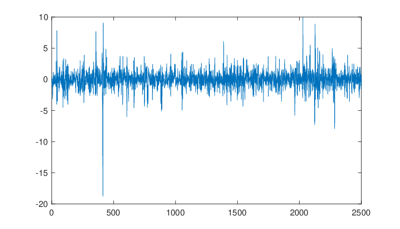
We have simulated 2500 sample from the proposed model (2.1)-(2.4) for two states, . Figure 2 shows the plot of the simulated time series and Table 1 reports some descriptive statistics of the simulated data.
Using the Bayesian inference, we estimate the parameters of the MS-STGARCH by applying the first 2000 samples. The prior density of each parameter is assumed to be uniform over a finite interval except for transition probabilities and which are drawn from some beta distribution. Table 2 demonstrates the true values of the parameters and also posterior means and standard deviations of the corresponding estimators over 10000 iterations, which 5000 of them are discarded as burn-in samples. The results of this table shows that the mean square errors (MSE) of the estimated parameters are adequately small. Using simulated data, we compare the in-sample fit and out-of-sample forecasting performance of the presented model with GARCH, STGARCH and MS-GARCH models in subsetions 5.1 and 5.2 respectively.
| Mean | Std. dev. | Skewness | Maximum | Minimum | Kurtosis | |
| Simulated data | -0.03 | 1.470 | -1.621 | 9.057 | -18.754 | 24.623 |
| True values | Mean | Std. dev. | MSE | |
|---|---|---|---|---|
| 0.300 | 0.314 | 0.031 | 0.0001 | |
| 0.200 | 0.224 | 0.022 | 0.0005 | |
| 0.050 | 0.12 | 0.014 | 0.0002 | |
| 0.500 | 0.510 | 0.049 | 0.002 | |
| 1.500 | 1.517 | 0.179 | 0.032 | |
| 1.900 | 1.750 | 0.09 | 0.008 | |
| 0.700 | 0.619 | 0.060 | 0.004 | |
| 0.100 | 0.094 | 0.016 | 0.0003 | |
| 0.250 | 0.217 | 0.021 | 0.0004 | |
| 0.500 | 0.619 | 0.013 | 0.0002 | |
| 0.970 | 0.982 | 0.093 | 0.009 | |
| 0.850 | 0.853 | 0.097 | 0.009 |
5.1 In sample performance analysis
| Model | SP 500 returns |
|---|---|
| GARCH | 5896 |
| ST-GARCH | 6021.4 |
| MS-GARCH | 5887.8 |
| MS-STGARCH | 5858.6* |
In order to compare the goodness of fit of the proposed model with GARCH, STGARCH and MS-GARCH, we apply the deviance information criterion (DIC) introduced by Spiegelhalter et al [37]. DIC is a Bayesian version of the reputable Akaike information criterion (AIC) that designed specifically for Bayesian estimation
that involves MCMC simulations, see [19] and [38] . The smallest DIC determines the best model. Berg applied DIC for the familiy of stochastic volatility (SV) models [9] and Ardia for the family of asymmetric GARCH models [5].
In the Markov-switching models, the likelihood is calculated by the following formula:
in which is the vector of all parameters in model and is obtained from (3.5). The deviance information criterion is computed as:
| (5.19) |
that is the posterior means of the vector . The results concerning DIC of the simulated data are reported in Table 3. It is apparent that the DIC of MS-STGARCH is the smallest value in the table. Thus our considered model has the best fit to the simulated data set among competing models.
5.2 Out-of-sample forecasting performance analysis
For appraising the performance of MS-STGARCH in forecasting, we survey the one-day-ahead value at risk (VaR) forecasts for the last 500 data of the simulated data. The one-day-ahead value at risk level , VaR is obtained by calculating the th percentile of the one-day-ahead predictive distribution (4.14). To test the VaR at level , we evaluate the sequence by
The out-of-sample VaR at level has good performance if the sequence are independent and obey the following distribution
The three likelihood ratio statistics for unconditional coverage (), independence () and conditional coverage () are as follows [13]:
1. LR statistic for the test of unconditional coverage,
where is the parameter of related Bernoulli distribution, which could be or , is the number of 1’s and is the number of 0’s in the series and .
2. LR statistic for the test of independence,
where is the number of transition from i to j () in the series, , and .
3.LR statistic for the test of conditional coverage,
has distribution with two degrees of freedom. When the value of is less than the critical value of distribution one infer that the conditional coverage is correct and there exist good VaR forecasts.
The results of the tests for simulation example are reported in Table 4. The second and third columns demonstrate the theoretical expected violations and the number of empirical violations respectively.
According to the results of Table 4, at the significance levels, as , the test is
rejected four times for GARCH and STGARCH, two times for MS-GARCH and one time for MS-STGARCH models.
For some risk levels the test of independence (IND test) is not applicable since no consecutive violations have been occurred. In such cases and so the statistic becomes infinity. The statistic at significance level is bigger than critical value for one case of GARCH and MS-STGARCH and also two cases of STGARCH. The conditional coverage (CC) test is higher than critical value with two degrees of freedom three times for the GARCH, four times for STGARCH, two times for the MS-GARCH and one time for the MS-STGARCH.
| Model | N | UC | IND | CC | ||
|---|---|---|---|---|---|---|
| 0.99 | 5 | 13 | 8.973 | 4.243 | 13.216 | |
| 0.95 | 25 | 42 | 10.195 | 1.756 | 11.95 | |
| 0.9 | 50 | 62 | 2.997 | 0.03 | 3.027 | |
| GARCH | 0.1 | 50 | 50 | 0 | 0.2664 | 0.2664 |
| 0.05 | 25 | 37 | 5.317 | 0.256 | 5.573 | |
| 0.01 | 5 | 12 | 7.111 | 1.15 | 8.263 | |
| 0.99 | 5 | 12 | 7.111 | 4.854 | 11.964 | |
| 0.95 | 25 | 38 | 6.181 | 1.527 | 7.706 | |
| 0.9 | 50 | 63 | 3.499 | 0.005 | 3.504 | |
| STGARCH | 0.1 | 50 | 53 | 0.197 | 0.030 | 0.227 |
| 0.05 | 25 | 39 | 7.102 | 0 | 7.103 | |
| 0.01 | 5 | 12 | 7.111 | 4.854 | 11.964 | |
| 0.99 | 5 | 13 | 8.970 | 0.914 | 9.887 | |
| 0.95 | 25 | 34 | 3.080 | 2.81 | 5.892 | |
| 0.9 | 50 | 56 | 0.773 | 0.558 | 1.330 | |
| MS-GARCH | 0.1 | 50 | 50 | 0 | 0.266 | 0.266 |
| 0.05 | 25 | 38 | 6.181 | 0.357 | 6.538 | |
| 0.01 | 5 | 10 | 3.914 | 1.75 | 5.665 | |
| 0.99 | 5 | 8 | 1.538 | NA | NA | |
| 0.95 | 25 | 36 | 4.510 | 3.987 | 8.498 | |
| 0.9 | 50 | 62 | 2.996 | 0.015 | 3.011 | |
| MS-STGARCH | 0.1 | 50 | 54 | 0.347 | 0.274 | 0.622 |
| 0.05 | 25 | 34 | 3.081 | 0.215 | 3.295 | |
| 0.01 | 5 | 9 | 2.613 | 2.126 | 4.739 |
| Mean | Std. dev. | Skewness | Maximum | Minimum | Kurtosis | |
| SP 500 | 0.023 | 1.287 | -0.337 | 10.957 | -9.469 | 14.049 |
6 Empirical data set
By applying daily log returns of the SP 500 for the period of 03/01/2005 to 03/11/2014 (2500 observations), we compare the performance of our model with the GARCH, MS-GARCH and ST-GARCH ones. From the 2500 observations of SP 500, the first 2000 observations are employed to estimate the parameters and the remaining 500 samples are used for forecasting analysis. Figure 3 plots the daily log returns in percentages11 1 log return in percentage is defined as , where is the index level at time t. of the SP500 indices.
In Table 5, the descriptive statistics of the log returns in percentages are presented. This table shows that the means are close to zero and there are some slightly negative skewness and excess kurtosis for the data set.

| MS-STGARCH | MS-GARCH | ST-GARCH | GARCH | ||||||
| Mean | Std.dev. | Mean | Std.dev | Mean | Std.dev | Mean | Std.dev | ||
| 0.194 | 0.001 | 0.233 | 0.004 | 0.336 | 0.011 | 0.269 | 0.005 | ||
| .276 | 0.008 | 0.278 | 0.012 | 0.421 | 0.019 | 0.120 | 0.007 | ||
| 0.085 | 0.006 | 0 | 0 | 0.121 | 0.016 | 0 | 0 | ||
| 0.289 | 0.003 | 0.320 | 0.009 | 0.364 | 0.014 | 0.439 | 0.004 | ||
| 2.345 | 0.132 | 0 | 0 | 2.206 | 0.218 | 0 | 0 | ||
| 0.717 | 0.087 | 0.779 | 0.012 | - | - | - | - | ||
| 0.677 | 0.007 | 0.430 | 0.011 | - | - | - | - | ||
| 0.365 | 0.013 | 0 | 0 | - | - | - | - | ||
| 0.264 | 0.015 | 0.207 | 0.007 | - | - | - | - | ||
| 1.097 | 0.017 | 0 | 0 | - | - | - | - | ||
| 0.986 | 0.004 | 0.994 | 0.003 | - | - | - | - | ||
| 0.985 | 0.005 | 0.991 | 0.004 | - | - | - | - | ||
| Coefficients | EGARCH | GJR-GARCH |
|---|---|---|
| Constant | 0.007 | 0.019 |
| arch effect | 0.127 | 0 |
| garch effect | 0.975 | 0.903 |
| leverage effect | -0.147 | 0.162 |
6.1 Estimation of the parameters
Applying the SP 500 set of samples and using the Bayesian MCMC method through Gibbs and griddy Gibbs sampling, we estimate the parameters GARCH, STGARCH, two-state MS-GARCH and MS-STGARCH to compare their performance. We also compare the proposed MS-STGARCH with EGARCH and GJR-GARCH. The prior density of transition probabilities and are drawn from the beta distribution and priors for the other parameters are assumed to be uniform over some finite intervals. We consider 10000 iterations of Gibbs algorithm which half of them are burn-in-phase. The posterior means and standard deviations for the parameters of the models corresponding to SP 500 data are reported in Table 6, which shows that the standard deviations are small enough in all cases, except for the slop parameter which relates to the state with low volatility.
The single-regime STGARCH has potential to react differently to negative and positive shocks but does not consider shifting between different levels of volatilities. The estimation results show that the level of volatility of the second regimes in MS-STGARCH and MS-GARCH are higher. This is by the fact that the coefficient for are respectively greater than . In Table 6, we see that the estimated parameters of the MS-STGARCH satisfies and , so the negative shocks have more affect on volatility than the positive shocks as , for for large negative shocks approaches to zero
Table 6 shows that the posterior means of transition probabilities ( and ) are close to one which indicate less switch between regimes. In Table 7 the estimated value of the parameters of EGARCH and GJR-GARCH are evaluated by applying the MLE method. Estimated conditional transition probabilities to the second state (high volatility regime), computed by (3.6) plotted in Figure 4.

| Model | SP 500 returns |
|---|---|
| GARCH | 8464.8 |
| ST-GARCH | 7513.5 |
| MS-GARCH | 7257.1 |
| MS-STGARCH | 7147.8* |
The MS-STGARCH has the potential to present better forecasting when different levels of volatilities are presented and there is different effect for negative and positive shocks. The results of Table 8 demostrates that the MS-STGARCH has the best fitting to data. For appraising the performance of MS-STGARCH in forecasting, we survey the one-day-ahead value at risk (VaR) forecasts for the samples of SP 500. Based on the last 500 returns (of SP 500 ), the out of sample VaR forecasts are calculated.

| Model | N | UC | IND | CC | ||
|---|---|---|---|---|---|---|
| 0.99 | 5 | 9 | 2.596 | 0.330 | 2.926 | |
| 0.95 | 25 | 26 | 0.038 | 2.740 | 2.778 | |
| 0.9 | 50 | 42 | 1.531 | 0.070 | 1.601 | |
| EGARCH | 0.1 | 50 | 32 | 8.227 | 0.001 | 8.228 |
| 0.05 | 25 | 12 | 8.790 | 1.155 | 9.946 | |
| 0.01 | 5 | 1 | 4.829 | 0.004 | 4.833 | |
| 0.99 | 5 | 10 | 3.891 | 0.408 | 4.299 | |
| 0.95 | 25 | 26 | 0.037 | 2.740 | 2.778 | |
| 0.9 | 50 | 42 | 1.531 | 0.070 | 1.601 | |
| GJR-GARCH | 0.1 | 50 | 31 | 9.236 | 0.036 | 9.239 |
| 0.05 | 25 | 16 | 3.925 | 2.775 | 6.700 | |
| 0.01 | 5 | 3 | 0.950 | 0.036 | 0.987 | |
| 0.99 | 5 | 9 | 2.596 | NA | NA | |
| 0.95 | 25 | 18 | 2.276 | 2.024 | 4.3 | |
| 0.9 | 50 | 44 | 0.830 | 0.252 | 1.082 | |
| GARCH | 0.1 | 50 | 42 | 1.395 | 0.071 | 1.466 |
| 0.05 | 25 | 27 | 2.276 | 0.142 | 2.418 | |
| 0.01 | 5 | 4 | 0.229 | NA | NA | |
| 0.99 | 5 | 5 | 0 | NA | NA | |
| 0.95 | 25 | 20 | 1.147 | NA | NA | |
| 0.9 | 50 | 31 | 9.235 | 0.5317 | 9.767 | |
| STGARCH | 0.1 | 50 | 28 | 12.684 | 1.191 | 13.875 |
| 0.05 | 25 | 8 | 16.441 | NA | NA | |
| 0.01 | 5 | 2 | 2.365 | NA | NA | |
| 0.99 | 5 | 8 | 1.526 | NA | NA | |
| 0.95 | 25 | 27 | 0.156 | 0.1787 | 0.335 | |
| 0.9 | 50 | 42 | 1.531 | 0.827 | 2.358 | |
| MS-GARCH | 0.1 | 50 | 37 | 4.112 | 0.252 | 4.364 |
| 0.05 | 25 | 15 | 4.926 | 0.539 | 5.465 | |
| 0.01 | 5 | 2 | 2.365 | NA | NA | |
| 0.99 | 5 | 9 | 2.596 | NA | NA | |
| 0.95 | 25 | 27 | 0.156 | 0.1787 | 0.335 | |
| 0.9 | 50 | 45 | 0.595 | 0.301 | 0.897 | |
| MS-STGARCH | 0.1 | 50 | 44 | 0.9 | 0.252 | 1.109 |
| 0.05 | 25 | 18 | 2.3 | 0.275 | 2.575 | |
| 0.01 | 5 | 2 | 2.38 | NA | NA |
According to the results of Table 9, at the and significance levels, the test is rejected three times for EGARCH, GJR-GARCH and STGARCH, two times for MS-GARCH and is accepted at all risk levels for the GARCH and MS-STGARCH models. The statistic at significance level is smaller than critical value with one degree of freedom for all cases that test is applied. Also excluding the cases of risk level 0.95 for the EGARCH and GJR-GARCH, the IND test is accepted at . At the significance level, the conditional coverage (CC) test is higher than critical value with two degrees of freedom two times for the EGARCH, GJR-GARCH and STGARCH while at the significance level this test is rejected three times for the EGARCH, two times for the GJR-GARCH and STGARCH and one time for the MS-GARCH.
In order to appraise the ability of competing models to forecast volatility, we apply the Diebold Mariano test. Testing for equal forecast accuracy is an approach to evaluate the predictive capability of competitor models. Diebold and Mariano (1995) proposed a unified method for testing the null hypothesis of no difference in the forecasting accuracy of two competing models [39]. Harvey, Leybourne and Newbold (1997) suggested a modified of Diebold Mariano (DM) test for small sample. The DM test or its HLN variant are applied widely in empirical forecasting research, see [16], [27] and [15]. Consider two forecast sequences as
and define
that are actual values. Let and
we would like to test the null hypothesis:
versus the alternative hypothesis
, under covariance stationarity of the process , the Diebold-Mariano (DM) statistic for testing the null hypothesis is given by:
and is approximately normally distributed for large samples. For evaluating the performance of our model in one-step ahead conditional variance forecast, we compute the DM statistic for pairwise comparison of MS-STGARCH model with GARCH, STGARCH, MS-GARCH,GJR and EGARCH models. According to the test results demonstrated in table 10, the null hypothesis is rejected at the significance level for all cases as all the statistics are less than . So our presented model has an improvement in the forecasting performance.
| Comparison of MS-STGARCH with | Statistic value |
|---|---|
| EGARCH | -3.89 |
| GJR-GARCH | -3.73 |
| GARCH | -3.84 |
| STGARCH | -4.08 |
| MS-GARCH | -2.08 |
Also for specifying the out of sample forecast performance of the MS-STGARCH toward the competing models, We compare the forecasting volatility , or conditional variance, of GARCH, STGARCh and MS-GARCH with the squared returns. In Figure 5, the squared returns of and the forecasting values of competing models are plotted. According to this figure the differences of forecast and real values (errors) in the MS-STGARCH always has been much less than other compared models. The results of Table 11 show that the least values of the MSE and MAE are related to the MS-STGARCH model that reveals the best forecast compared with the other reviewed models in this paper.
| Model | Mean square error (MSE) | Mean absolute error (MAE) |
|---|---|---|
| EGARCH | 0.676 | 0.528 |
| GJR-GARCH | 0.665 | 0.517 |
| GARCH | 0.707 | 0.524 |
| ST-GARCH | 0.384 | 0.498 |
| MS-GARCH | 0.302 | 0.395 |
| MS-STGARCH | 0.227* | 0.369* |
7 Conclusion
Applying Markov switch structure cause to have a better fitting while the existence of different levels of volatilities are evident. Also the asymmetry effects of negative and positive shocks in many case are trivial and transition between this effects happens in some smooth ways and not sudden. So in many cases the use of MS-STGARCH has advantages to the other methods as GARCH, MS-GARCH, ST-GARCH, EGARCH and GJR-GARCH as we find this performance for SP500 indicies where studied in the paper. In such cases a much better fit to the data can be provided by the presented model which leads to the forecasts with much smaller error. The MS-STGARCH extends the MS-GARCH model by considering convex combination of time dependent logistic weights between the effect of negative and positive shocks in each regime. It also extends the STGARCH model by considering transition between different levels of volatilities. We show that the existence of a simple condition suffices for the existence of an asymptotic upper bound for the second moment of returns which causes the stability of the model.
By fitting the GARCH, STGARCH, MS-GARCH and MS-STGARCH models to the SP 500 log returns we find that our model has the best DIC, see Table 8, and provides the best forecast volatilities, see Figure 5. Also in performing Diebold Mariano test, our model has the best performance in compare to the EGARCH and GJR-GARCH. The forecasted one-day ahead Value at Risk (VaR) of our model has better performance to the EGARCH,GJR-GARCH, STGARCH and MS-GARCH.
Further researches could be oriented to investigate the existence of the third and the fourth moments of the process and derive the necessary and sufficient conditions for stationarity and ergodicity of the process. For the sake of simplicity it was assumed that the process conditional mean is zero, this assumption could be relaxed by refining the structure of model to allow ARMA structure for conditional mean. Since Financial time series data are typically observed to have heavy tails [31], it might be interesting to replace the Gaussian distribution with Student’s t or stable Paretian distributions to investigate the ability for modeling heavy tailed property of financial time series such as [14] work.
Appendix A
Proof of Remark 3.1.
As the hidden variables have Markov structure in MS-STARCH model, so
| (7.20) |
Appendix B
Proof of Theorem 3.1.
Let denotes the expectation with respect to the information up to time t. Thus the second moment of the model can be calculated as, see [1]:
| (7.21) |
Also let and denote and , respectively, where is the realization of the state at time t. Applying to the method of Medeiros [33], we find an upper bound of , for by the following
| (7.22) |
The term (II) in (7.22) can be interpreted as follows:
| (7.23) |
where is the support of .
Upper bound for III in (7.22):
Let be a constant, so
in which
As by (2.4), and so
also
by (2.4),
| (7.24) |
So for any fixed positive small number , we can consider so large that for , and for , . Hence
Since the distribution of the is symmetric, then
and
Therefor
Upper bound for IV in (7.22):
| (7.25) |
By replacing the obtained upper bounds and relations (7.23) in (7.22), the upper bound for is obtained by:
| (7.26) |
in which by Bayes’ rule
where is the transition probability matrix.
Let , be a -by-1 vector and consider be a vector that is made of K vector . By (7.23)-(7.26), the following recursive inequality is attained,
| (7.27) |
with some initial conditions The relation (7.27) implies that
| (7.28) |
Following the matrix convergence theorem [30], the necessary condition for the convergence of when is that . Under this condition, converges to zero as t goes to infinity and converges to provided that matrix is invertible. So if ,
By (7.21) the upper bound for the asymptotic behavior of unconditional variance is given by
Acknowledgement: This paper initiated during Professor Rezakhah sabbatical at Institute of Mathematics at the EPFL where benefitted from the discussion of the paper with Professor Stephan Morgenthaler and careful written comments and suggestions of Professor Anthony Davison which caused to improve the quality of this paper.
References
- [1] Abramson A, Cohen I (2007) On the stationarity of Markov-Switching GARCH processes. Econometric Theory 23:485-500
- [2] Alemohammad N, Rezakhah S, Alizadeh SH (2016) Markov switching component GARCH model: stability and forecasting. Commun Stat Theory and Methods 45(15):4332-4348
- [3] Alizadeh SH, Rezakhah S (2013). Hidden Markov mixture autoregressive model: stability and moments. Commun Stat Theory and Methods 42:1087-1104
- [4] Ardia D (2008) Financial Risk Management with Bayesian Estimation of GARCH Models: Theory and Applications, Volume 612: Lecture Notes in Economics and Mathematical Systems. Heidelberg, Germany: Springer
- [5] Ardia D (2009) Bayesian estimation of a Markov switching threshold asymmetric GARCH model with Student-t innovations. Econometrics journal 12(2):105-126
- [6] Bauwens L, Lubrano M (1998) Bayesian inference on GARCH models using the Gibbs sampler. Econometrics journal 1:23-46
- [7] Bauwens L, Storti G (2009) A component GARCH model with time varying weights. Studies in Nonlinear Dynamics and Econometrics 13 Article 1
- [8] Bauwens L, Preminger A, Rombouts VK (2010) Theory and inferencefor Markov switching GARCH model. Econometrics journal 13:218-244
- [9] Berg A, Meyer R, Yu J (2004) Deviance information criterion for comparing stochastic volatility models. Journal of Business and Economic Statistics 22:107-120
- [10] Black F (1976) studies in stock price volatility changes. Proceedings of the American Statistical Association, Business and Economics Statistics pp:177-181
- [11] Bollerslev T (1986) Generalized autoregressive conditional heteroscedasticity. Journal of Econometrics 31:307-327
- [12] Chib S (1996) Calculating posterior distributions and model estimates in Markov mixture models. Journal of Econometrics 75:79-97
- [13] Christofferssen P (1998) Evaluating interval forecasting. International Economic Review 39:841-862
- [14] Curto JD, Pinto JC, Tavares GN (2009) Modeling stock markets volatility using GARCH models with Normal, Students t and stable Paretian distributions. Statistical Papers 50:311-321
- [15] Curto JD, Pinto JC (2012) Predicting the financial crisis volatility. Economic Computation And Economic Cybernetics Studies and Research Journal 46:183-195
- [16] Diebold FX, Mariano RS (1995) Comparing predictive accuracy. Journal of Business and Economic Statistics 13:253-263
- [17] Engle RF (1982) Autoregressive conditional heteroscedasticity with estimates of the variance of united kingdom inflation Econometrica 50:987-1007.
- [18] Engle RF (1990) Discusion: stock volatility and the crash of ’87. Review of Financial Studies 3:103-106
- [19] Gelman A, Hwang J, Vehtari A (2014) Understanding predictive information criteria for Bayesian. Statistics and Computing 24:997-1016
- [20] Glosten LR, Jagannathan R, Runkle D (1993) On the relation between the expected value and the volatility of the nominal excess return on stocks. Journal of Finance 48:1779-1801
- [21] Gonzalez-Rivera G (1998) Smooth transition GARCH models. Studies in Nonlinear Dynamics and Econometrics 3:61-78
- [22] Gray SF (1996) Modeling the conditional distribution of interest rates as a regime-switching process. Journal of Financial Economics 42:27-62
- [23] Grimmett G, Stirzaker D (2001) Probability and random processes. Oxford University press, New York
- [24] Haas M, Mittnik J, Paolella MS (2004) A new approach to markov-switching GARCH models. Journal of Financial Econometrics 2:493-530
- [25] Haas M Krause J, Paolella MS, Steudc SC (2013) Time varying mixture GARCH models and asymmetric volatility. The North American Journal of Economics and Finance 26:602-623
- [26] Hamilton JD, Susmel R (1994) Autoregressive conditional heteroskedasticity and changes in regime. Journal of Econometrics 64:307-333
- [27] Harvey D, Leybourns S, Newbold P (1997) Testing the equality of prediction mean squared error. International Journal of Forecasting 13:281-291
- [28] Kaufman S, Fruhwirth-Schnatter S (2002) Bayesian analysis of switching ARCH models. Journal of Time Series Analysis 23:425-458
- [29] Klaassen F (2002) Improving GARCH volatility forecasts with regime-switching GARCH. Empirical Economics 27:363-394
- [30] Lancaster P, Tismenetsky M (1985) The theory of matrices, 2nd ed. Academic press
- [31] Liu S, Heyd CC, Wong WK (2008) On estimation in conditional heteroskedastic time series models under non-normal distributions. Statistical Papers 49:455-469
- [32] Lubrano M (2001) Smooth transition GARCH models: a Bayesian approach mixture models. Recherches Economiques de Louvain 67:257-287
- [33] Medeiros MC, Veiga A (2009) Modeling multiple regimes in financial volatility with a flexible coefficient GARCH(1,1). Journal of Econometric Theory 25:117-161
- [34] Miazhynskia T, Dorffner G (2006) A comparison of Bayesian model selection based on MCMC with an application to GARCH-type models. Statistical Papers 47:525-549
- [35] Nelson DB (1991) Conditional heteroskedasticity in asset returns: a new approach. Journal of Econometrica 59:347-370
- [36] Ritter C, Tanner MA (1992) Facilitating the Gibbs sampler: The Gibbs Stopper and the Griddy-Gibbs Sampler. Journal of the American Statistical Association 87:861-868
- [37] Speigelhalter DJ, Best NG, Carlin BP, Van del lindle A (2002) Bayesian measures of model complexity and fit. Journal of the Royal Statistical Society, Series B 64:583-639
- [38] StataCrop (2015) Stata: release 14 Statistical software. College station, TX: StataCrop LLC
- [39] Xekalaki E, Stavros D (2010) ARCH nodels for financial applications. New York, Wiley
- [40] Zakoian JM (1994) Threshold heteroskedastic models. Journal of Economic Dynamic and Control 27:577-597