Combined Analysis of Amplitude and Phase Variations in Functional Data
Abstract
When functional data manifest amplitude and phase variations, a commonly-employed framework for analyzing them is to take away the phase variation through a function alignment and then to apply standard tools to the aligned functions. A downside of this approach is that the important variations contained in the phases are completely ignored. To combine both of amplitude and phase variations, we propose a variant of principal component analysis (PCA) that captures non-linear components representing the amplitude, phase and their associations simultaneously. The proposed method, which we call functional combined PCA, is aimed to provide more efficient dimension reduction with interpretable components, in particular when the amplitudes and phases are clearly associated. We model principal components by non-linearly combining time-warping functions and aligned functions. A data-adaptive weighting procedure helps our dimension reduction to attain a maximal explaining power of observed functions. We also discuss an application of functional canonical correlation analysis in investigation of the correlation structure between the two variations. We show that for two sets of real data the proposed method provides interpretable major non-linear components, which are not typically found in the usual functional PCA.
Keywords: Functional data; principal component analysis; amplitude variation; phase variation; manifold; exponential map.
1 Introduction
Functional data are frequently encountered in modern sciences (Ramsay and Silverman, 2005). When functional data consist of repeated measurements of a common activity or development over time, they often show a similar pattern of progression, which can be understood as a combination of two types of variations, called amplitude and phase variations. When the phase variation resides in functional data, a naive application of standard tools such as the pointwise mean and variance, and functional principal component analysis (FPCA) tends to yield misleading results (Gasser et al., 1984). Curve registration (or function alignment) has been routinely performed to disregard the phase differences (Kneip and Ramsay, 2008, cf.). Recently, several researchers have pointed out that the phase variation also contains important information (Kurtek et al., 2013; Tucker et al., 2013; Hadjipantelis et al., 2015; Hadjipantelis et al., 2014; Marron et al., 2015).
A prominent example where the phase variation is commonly observed is growth curves (Chen and Müller, 2012; Park and Ahn, 2017). For example, the growth rate curves from the well-known Berkeley study (R.D.Tuddenham and Snyder, 1954) share common events such as pubertal growth spurt and maturity. Visual inspection of this data set reveals that the curves develop the events with varying magnitudes of heights (amplitude variation), and at varying temporal paces (phase variation), as shown in in Fig. 1. Moreover, these two types of variations are clearly associated to each other; individuals who reach the phase of pubertal growth spurt (corresponding to the main peak of curves) later in their ages tend to show smaller maximum pubertal growth rates. This important major association is not captured in the application of FPCA to the original data or to the aligned data (see Fig. 1(b) and (c)).
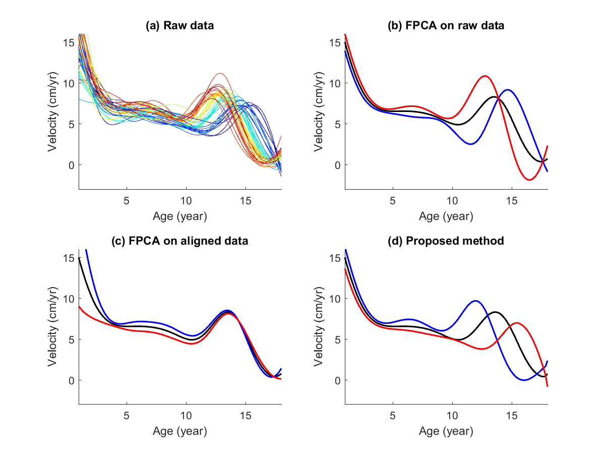
In this paper, we propose a principal component analysis for the original, unregistered data, combining the two types of variations into one. The principal components (PCs) obtained from the proposed method, which we call functional combined principal component analysis (FCPCA), effectively capture all of the amplitude and phase variations, including their associations. In Fig. 1, an advantage of FCPCA is exemplified for the growth data, where the dominant association between the amplitude and phase variations is well-captured in the first combined PC.
We assume that the observation is composed of an amplitude function, , and a time-warping function, , and that the observed functions can be well-aligned by time-warping functions. Our method is developed for a particular class of time-warpings, denoted by , consisting of orientation-preserving diffeomorphisms of the unit interval , as developed and used in Srivastava et al. (2007); Srivastava et al. (2011); Kurtek et al. (2013); Tucker et al. (2013); Yu et al. (2017). For the combined analysis of amplitude and phase functions, we further define a bijection, denoted by , between and a convex subset of the function space. This step enables us to use the standard linear functional operations to . In our FCPCA framework, we assume that the combined random function can be represented as a linear combination of orthogonal functions. The Karhunen-Loève transformation of this function is simply the FPCA in the combined function space, the components of which are then mapped back to the original function space (in which lies). For estimation of the functional combined components, we use a function alignment method to obtain predictions of and , denoted by and . The resulting functions and are then joined together, to which a standard functional PCA is applied. These two functions are adaptively weighted so that the resulting combined PCs achieve the maximal explaining power of the observed functions. The result is represented and visualized in the original function space, which can be used to aid interpretation of each principal component.
We also demonstrate a use of the functional canonical correlation analysis in the detection of maximally correlated components between the amplitude and phase functions.
In recent years, there have been a few attempts to analyze the phase variations. In particular, the phase variations are used in segmentation of periodic signals (Kurtek et al., 2013), clustering (Sangalli et al., 2010), functional regression (Gervini, 2015; Hadjipantelis et al., 2015; Hadjipantelis et al., 2014) and classification (Tucker et al., 2013). In Srivastava et al. (2011); Yu et al. (2017); Kurtek et al. (2013); Tucker et al. (2013), the Fisher-Rao function alignment is used to obtain time-warping functions, and the authors suggest several different approaches of analyzing the phase variation through the time-warping functions. They, however, did not discuss the association between two types of variations. While we use the Fisher-Rao alignment as used in Tucker et al. (2013), the “composite FPCA” of Tucker et al. (2013) is less efficient than our proposal when the amplitude and phase functions are linearly associated. Analyses combining the phase and amplitude variations have been reported more recently in Hadjipantelis et al. (2015), where the authors used a log transformation for phase functions (thus making use of compositional data analysis). In contrast, we use the transformation to take advantage of the well-developed tools of conventional functional data analysis. Moreover, Hadjipantelis et al. (2015) used a linear functional model consisting of individual principal component scores from each of amplitude and phase functions, which can be viewed as a two-step approach. In contrast, we directly combine the two functions using data-adaptive weights, for the purpose of dimension reduction through non-linear principal components. Finally, Chen and Müller (2012) proposed a nonparametric dimension reduction using manifold learning. Our model-based approach is conceptually different from the nonparametric approach of finding nonlinear submanifolds in Chen and Müller (2012).
The rest of the paper is organized as follows. In Section 2, we formally define a population structure to model the amplitude, phase and their association, and introduce our two models, functional combined PCA and CCA. Estimation of the model parameters and the data-adaptive choice of weights are discussed in Section 3. In Section 4, the advantages of the proposed methods are demonstrated in analyses of two real data sets, and in Section 5 several simulation studies are reported.
2 Models
2.1 Decomposition into two variations
We consider a smooth random function that inherently contains amplitude and phase variations and is composed of two random functions and :
| (1) |
We restrict the domain of to be without losing generality. The amplitude function is assumed to be a smooth square-integrable function on , i.e., . The time-warping function is an orientation-preserving diffeomorphism on and lies in
In other words, is the set of cumulative distribution functions of absolutely continuous random variables with support on . Note that the endpoint constraints restrict the warping of to only occur on the given interval, and the positive derivative constraint does not allow the warps travel back into the past. For any , the inverse function exists, and is also a member of . This implies that . We assume that the identity function is the center of the random warping function, where the center is defined later in Section 2.2. This assumption formally defines phase variation as the deviation of from the identity. This choice of center is purely for the sake of simplicity and interpretability; our analysis using the Fisher-Rao function alignment and the transformation of discussed in Section 2.2 is in fact insensitive to different choices of the center (Marron et al., 2015, cf. ).
2.2 Simplifying the geometry of
Working directly with warping functions is not desirable since is not convex; there exist and such that and . Thus, standard operations based on Euclidean geometry can only be applied with great care. We circumvent this issue by adopting the geometric approach laid out in Srivastava et al. (2011); Tucker et al. (2013), and introduce a bijection , where is a convex subset of containing the origin (i.e., the function), so that standard operations can be employed. The map is defined below in (4), and its inverse in (6). The map is best understood as a composition of two transformations, as elaborated below.
Mapping to the unit sphere:
The level of difficulty in dealing with is eased by taking the square-root of the derivative of , the operation of which is denoted by ,
| (2) |
This corresponds to the “sqaure-root velocity function” of Srivastava et al. (2011). Denote by the positive orthant of the unit sphere in . It can be checked that for any , and that is a bijection. A significant benefit of using this transformation is that the complicated structure of is simplified to that of the well-known unit sphere.
The “center” of the random diffeomorphism is defined through the Karcher mean (Karcher, 1977) of . Let
be the Karcher mean using the geodesic distance . Then is the center of .
Mapping to a tangent space:
The positive unit sphere has been well-studied as a space for random directions and unit-norm random functions. While there are several approaches of modeling random elements in (Mardia and Jupp, 2000; Jung et al., 2012; Tucker et al., 2013, cf.), we use a linear approximation of by a tangent space. The tangent space approximation is schematically illustrated in Fig. 2. For simplicity, we use the unit sphere that includes .

The tangent space of at a point , denoted by , is the collection of functions in orthogonal to ,
where is the usual inner product in . Functions in will be approximated by functions in . Figure 2(b) schematically illustrates and the approximation of the -valued function by the function ; see (3). To help understand the tangent space approximation, we take the hyperplane in tangent to at . The tangent space is obtained by a translation of the hyperplane so that the tangent point is translated to the origin. Thus, is a subspace of .
Points (i.e., functions) on the tangent space can provide good approximations of functions in a subset containing . In particular, the log map is frequently used for such approximation, and is defined as ,
| (3) |
The geodesic distance measures the distance between and by the length of the shortest arc on that joins and . When the standard -norm is used for , the geodesic distance between and and the direction in which shoots from , for any , are preserved by the log map.
A sensible choice of the tangential point is given by the assumption that is the center of . It can be seen that for all . Thus we choose the constant function as . This entails that the Karcher mean of is , and that . Note that the center, , of is in general different from the mean of .
Summary:
The mapping we use for the trasformation of the time-warping function is ,
| (4) |
where . We call phase function. Since the image of (denoted by ) is a convex subset of , standard vector operations (e.g., the Gram-Schmidt operations) can be used for the phase function .
2.3 Construction of by the amplitude and phase functions
Any pair of amplitude and phase functions can be composed to a single function, by reverting the decomposition in Sections 2.1 and 2.2. To define this composition, we note that the log map is indeed the inverse of exponential map, , defined by
| (5) |
For any phase function , the corresponding time-warping is uniquely given by
| (6) |
that is, , . All in all, any random functions can be composed to yield a random function in the form of (1) as follows.
| (7) |
2.4 Models for joint variability of amplitude and phase functions
In this section, we define the joint population structures of the amplitude and phase functions . The parameters we aim to estimate are defined in the models we describe below. Recall that the mean of corresponds to the identity time-warping and thus .
2.4.1 Model for functional combined principal components
To model the association between and , we define a random function on the extended domain for a positive scaling parameter ,
| (8) |
The exclusion of the end point of the domain of in the construction of does not lose any information since is assumed to be continuous. Note that for any , we have . The parameter is introduced to adjust scaling imbalance between and . We will discuss the role of shortly, but for now we let be fixed.
For a given , denote the eigen-decomposition of the covariance function of by
where are eigenvalues of in the decreasing order (, ), and is the eigenfunction corresponding to . The eigenfunctions are orthonormal, i.e., and for . The superscript is used to emphasize the dependence of the decomposition on . By Karhunen-Loéve decomposition, we write , , where ’s are uncorrelated mean-zero random variables with . Note that the mean function does not depend on since is irrelevant of and . The function is then divided into the amplitude and phase functions as
| (9) |
In (9), the joint variation between and is paired in eigenfunctions .
The role of the scaling parameter in (8) becomes clear from (9). As opposed to the unit-free , values of depend on the unit in which measurements of (or ) are made. The overall analysis should not depend on the particular scaling of (due to, for example, changes from the metric system to US customary units). Since scaling of by is equivalent to scaling of by , we introduce the scaling parameter applied only to the “ part” of , in order to keep the original unit of observed (and ). The eigenfunctions and their eigenvalues vary for different choices of ; for a small , the first few eigenfunctions are bound to capture more variations from the amplitude variation, while for a large , the leading eigenfunctions reflect more phase variations. For any given , or the pair , there exists a continuum of different sets , depending on the value of , which causes an identifiability issue. To our aim of succinctly representing the combined variation of and in the original function space, we choose to be dependent on the original random function as discussed below.
Let be a positive integer. From (7) and (9), for a given , we define as a projection of onto the -dimensional eigen-space, spanned by the first eigenfunctions, by
| (10) |
where for ,
| (11) |
This projection utilizes the standard orthogonal projection of to its eigen-space in , but is non-linear in the original function space . To minimize the approximation error of with respect to , the scaling parameter is chosen as follows:
| (12) |
where is a distance function on . We use for fast computation and mathematical convenience. Other distance functions such as -distance, Fisher-Rao distance (Srivastava et al., 2011), and the earth-mover’s distance (Rubner et al., 2000) can be used as well.
For a chosen , the combined principal component of and (or the so-called eigen-mode) can be visualized in the original function space. In particular, the th mode of variation of can be visualized by overlaying the curves for various values of . Here, and are obtained from (9) by setting and also setting for all . Figure 1(d) shows empirical estimates of , , for the Berkeley data. Our estimation procedure is described in Section 3.
We note that one may use approaches of multivariate functional principal component analysis (Chiou et al., 2014; Happ and Greven, 2016, cf.) instead of gluing the two functions as done in (8). While such multivariate approaches may be mathematically more appealing, using (8) facilitates our discussion for the adaptive choice of , and is satisfactory in our numerical examples.
2.4.2 Model for correlation analysis
As another approach to model the association between and , we briefly discuss a model for a functional combined canonical correlation analysis (CCA).
For a pair of non-random functions , write for the correlation coefficient between two random variables and . Here, and are the random amplitude and phase functions as defined before. In functional combined CCA, the association between the amplitude and phase functions is modeled by a few canonical weight function pairs that sequentially maximize . In general, the th canonical weight function pair maximizes , with the constraint that for . The correlation coefficient is called the th canonical correlation coefficient.
The joint variation modeled by the th canonical weight functions and can be visualized in the original function space. For , let
| (13) |
Then the th mode of variation given by the functional combined CCA is visualized by overlaying the curves of for various values of . A reasonable choice of satisfies , where is the slope from the regression of against
3 Estimation
In this section we discuss our procedures for the application of functional combined PCA and CCA to a data set.
3.1 Decomposition into amplitude and phase functions
Let , , be the th realization of the underlying random function obtained from independent experiments. The realizations ’s do not manifest themselves in a direct way. They are usually recorded at discrete time points, leading to observed values , at time point index , and sometimes are blurred with measurement errors. We assume that smoothing the observations with a suitable basis function system gives a close approximation of . Denote the approximations to by , .
Each is then decomposed into the amplitude and phase functions by applying the method of Fisher-Rao function alignment (Srivastava et al., 2011) to all sample , which iteratively time-warps to a template function, resulting in the time-warp and the aligned function , satisfying
| (14) |
Write . The Fisher-Rao alignment is known to be invariant to the choice of templates, and we choose it to satisfy so that the center of is . Other methods of function alignment may be used here. We use the method of Srivastava et al. (2011) for its good performance (Kurtek et al., 2013; Marron et al., 2015) and invariance to the choice of templates.
3.2 Functional combined PCA
In the model for the functional combined PCA, the population eigen-structure depends on the unknown parameter . We first discuss the empirical eigen-decomposition for any given , and then present our procedure to obtain a data-adaptive estimate of .
3.2.1 Estimation of
Let the scaling parameter be given. For easy computation, we evaluate the functions and on a fine grid, , to obtain their vector expressions and . Write
and let . The eigen-decomposition of the sample covariance matrix obtained from provides pairs of eigenvalues and eigenvectors ,
where , and for . Estimates of and of are obtained by interpolation of the elements of and .
3.2.2 Estimation of
The estimates are dependent on the value of . We note that the true parameter depends on the number of principal components, , used in (12). For the purpose of exploratory analysis and visualization of the data, is typically chosen as a small number. For a given , our strategy in the estimation of is to use an empirical minimizer of (12). For this, let be the th score of the th observation. We write for an approximation of the th observation by the first empirical principal components, which is defined by (10), by replacing and with
Our choice of is then
| (15) |
which entails that the first combined principal components found at reconstruct most faithfully, compared to other values of . In practice, we use a numerical method to solve (15), which is almost instantaneous for small values of .
In all of our numerical studies, the minimizer always exists, and does not degenerate to 0 nor diverges to infinite. Heuristically, this is because we assume that the observation has both amplitude and phase variations. Large (or small) values of force the eigenfunctions to explain only the phase variation (or amplitude variation, respectively). For large , the amplitude variation of is typically not found in ; for small , the two functions and exhibit different phases.
3.3 Functional combined CCA
In the functional combined CCA of the data , we again use the decomposed functions , obtained in Section 3.1, to compute estimates of the triple as defined in Section 2.4.2.
It is well know that a naive adaptation of the usual CCA procedure to functional data often leads to spurious estimates of the triple with the estimated canonical correlation coefficient close to one. Following the suggestions in Leurgans et al. (1993), we use the regularized functional CCA as follows. For a given smoothing parameter , the estimates of the canonical weight functions are
| (16) |
subject to , where and denote sample covariance and variance and is the second order differential operator. Subsequent pairs are obtained similarly with the additional orthogonality constraint. The th empirical canonical correlation coefficient is given by the sample correlation coefficient of . We refer to Ramsay and Silverman (2005) for a detailed procedure of the functional CCA and the choice of by a generalized cross-validation.
4 Combined analysis of amplitude and phase variations in real data sets
In this section, we illustrate applications of the proposed methods to two sets of real data.
4.1 Berkeley growth data
The Berkeley growth data set (R.D.Tuddenham and Snyder, 1954) consists of the height measurements of 39 boys and 54 girls from age 1 to 18. We present here the results of our analysis for the boy-only data. The analysis for girls’ growth leads to a similar conclusion. To highlight periods of slower and faster growths, we use the growth velocity curves, by taking derivatives of the smoothed growth curves. These raw data are shown in Fig. 1(a).
The application of the proposed functional combined PCA and CCA results in a succinct dimension reduction of the data, as well as interpretable major modes of variations. In particular, the first two combined principal components (PCs) well explain the association between growth velocities (amplitude variation) and temporal paces (phase variations).
The mode of variation captured in the first combined PC explains the pattern that boys with higher overall growth rates tend to have fast temporal paces (e.g., reaching their pubertal growth spurt earlier than others). In the first row of Fig. 3, the red curves represent this patten. On the other hand, boys with lower growth rates tend to have slower paces, as shown in the figure by the blue curves. The second combined PC (shown in the second row of Fig. 3) captures a contrast, which is characterized by the growths before and after about 9 years old. Specifically, the second PC explains a growth pattern that the growth rate and pace are positively associated for growths in ages 0–9, and negatively associated for growths in ages 10–18. As mentioned earlier, FCPCA aims to simultaneously capture the amplitude, phase and their association, and does so for this data set. The interpretable modes of variation shown in Fig. 3 are not typically found in applications of functional PCA (see e.g. Fig. 1).


An application of our functional combined CCA to the data set reveals a difference between two of our proposed methods. The reconstructed functions from the most correlated components are shown in the botton row of Fig. 4. These are visually different from the combined principal components shown in the top row. The differences in patterns found by functional combined PCA and CCA should not be surprising. The internal variations within each of amplitude and phase functions affect the combined PCA, while, in CCA, they are simply ignored.
4.2 Lip motion data
The data set we analyze here is a part of lip motion data used in Ramsay et al. (1996). The data set is composed of measurements at 51 equally-spaced points in the timeframe from 0 to 340 milliseconds of a vertical position of lower lip while the subject speaks a syllable “bob” 20 times. The dynamics of lip motion is well captured by its acceleration. These second derivatives plotted in Figure 5(a) show a common pattern. Lip movement is first accelerated negatively and then pass through a positive acceleration phase during which the descent of the lower lip is stopped. This lip opening phase is followed by a short period of near zero acceleration when pronunciation of the vowel “o” is at its full force, followed by another strong acceleration upward initiating lip closure. The movement is completed by a negative acceleration episode as the lip returns to the closed position (Ramsay et al., 1996).

By an application of FCPCA, we found that the first combined PC explains a large portion (58%) of the total variation. The first mode of variation, shown in Figure 5(b), explains a speech habit of the speaker; as he makes the sound of the word louder (or softer), he tends to speak faster (or slower, respectively). For this data set, the findings from the function combined CCA are similar to those of FCPCA.
5 Numerical studies
5.1 Efficiency of functional combined PCA under non-linear associations
The success of the proposed methods depends on whether a particular type of the association between the amplitude and phase variations exists in data. In particular, our methods are well-suited for a linearly dependent amplitude and phase functions. To elaborate this point, we present a toy data analysis.
Two sets of data are prepared by sampling from the amplitude and phase function pair . We have set each of and has one major principal component, and the association between the PC score of and that of is either nearly linear or severely non-linear (quadratic). The observations are obtained by the composition, , and displayed in the first column of Fig. 6. The types of association, or the degrees of non-linearity, are illustrated in the scatters of the two individual PC scores, shown in the second column of Fig. 6. The proposed functional combined PCA works well for the first data set, where the association between and is nearly linear.
To confirm this and to investigate the sensitivity of our method to the degrees of non-linearity, we evaluate for each data set the mean squared approximation error (MSE) using only the first components, as a function of , computed by . These errors are compared with errors from other natural competitors: the usual functional PCA (FPCA) and a composite functional PCA, proposed in Tucker et al. (2013). The FPCA is applied to the original data (without applying function alignment), and the first components are used to approximate the observations. In the composite method, the FPCA is applied to each individual functions ( and ). First components from both and are used to approximate the observations (thus using components). These MSEs are shown in the last column of Fig. 6.
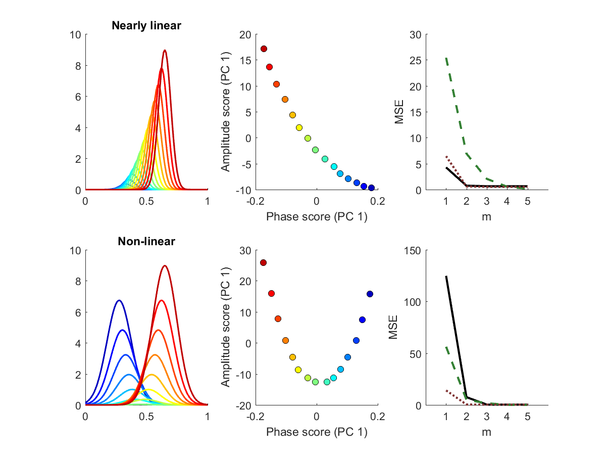
Note that our definition of one-dimensional linear or nearly linear association, as shown in the first row of Fig. 6, typically results in a one-dimensional non-linear mode of variation in the original function space. This non-linear variation is not completely captured in a single component of FPCA, and oftentimes needs multiple components. In contrast, our method efficiently captures the non-linear variation (showing the smallest MSE for ), since in fact, the non-linear association becomes linear in and . For this type of association, the usual FPCA needs several components to capture the non-linear variation in the original space, and is less favorable. The separate method, on the other hand, uses linear components (compared to only components in the other two methods), thus is expected to show better performances than FPCA in general. Note that our functional combined PCA has smaller errors than the separate method has for this data set.
As the degrees of non-linearity intensify, the advantage of the functional combined PCA gradually lessens. For the severely non-linear case (shown in the second row of the figure), our method fails to capture the non-linear mode of variation in one component. However, it performs comparable to other methods when more than one component is used, i.e. for .
5.2 Performance of estimation in functional combined PCA
In this and next subsections, we exhibit good performances of our estimation procedures. The success of our methods is largely dependent upon the quality of the alignment. The Fisher-Rao function alignment we choose to use has been shown to work well in practice (Kurtek et al., 2013), but its theoretical results (e.g., consistency in the estimation of ) are limited (Srivastava et al., 2011). Instead, we use simulated data sets to glimpse the consistency of the estimators. We have tried a range of parameter settings, and the results are concordant across settings. Below we present representative cases.
We use a four-component model for (8), where , . We set , , where is the density function of the standard normal. The eigenfunctions for amplitudes are chosen by the Gram-Schmidt orthogonalization of four functions
while the eigenfunctions for phases are from . Figure 7 illustrates the mean function, and the eigenfunctions. We set and . The scores are sampled from the standard normal distribution. The observed function is obtained from using (7) and (9). An example of such random sample is shown in the left panel of Fig. 7.
We observe at each time point , for with measurement error . As for a smoothing step for ’s, the B-spline basis system of degree 4 with a roughness penalty on second derivative is used. Following de Boor (2001), knots are placed at evaluation points and, following Craven and Wahba (1979), the value of the smoothing parameter is determined by the generalized cross-validation method.

For sample sizes , we generated from the model described above and obtained the estimates , from our procedure discussed in Section 3.2. For a random sample of size , the analysis result is shown in Fig. 8. There, we see that the first two component estimates capture the amplitude, phase and their association rather well; the estimates are very close to the population eigenfunctions, shown in Fig. 7. The third component seems negligible as is small.

We repeat the experiment 100 times to witness the sampling distributions of the estimators. The result is summarized in Table 1. We observed that the estimators approach their population counterparts as the sample size increases.
| () | 1.44 (0.31) | 1.28 (0.29) |
|---|---|---|
| () | 4.12 (0.26) | 3.81 (0.21) |
| () | 2.98 (0.37) | 2.74 (0.18) |
| 2.89 (1.27) | 2.15 (0.85) | |
| 0.49 (0.24) | 0.38 (0.36) | |
| 0.71 (0.41) | 0.34 (0.50) |
5.3 Performance of estimation in functional combined CCA
For a model for the functional combined CCA, the amplitude and phase functions are each modeled using four principal components, where , , , so that the corresponding function is obtained by the function composition (7). We use , , as shown in Fig. 7. We choose to model only one canonical weight function pair by setting with the canonical correlation coefficient 0.8. (That is, only the first “y” component and the second “x” component are correlated.) The variances of individual principal components are set to be , and . The scores are independently sampled from , except that . The random function is observed at a dense grid with a measurement error drawn from and the data are processed as done in Section 5.3.
We obtained the empirical sampling distributions of the estimators for sample sizes with 100 repetitions. The results, summarized in Table 2, suggest a good performance of our estimation procedure. Note that we have used the generalized cross validation (Ramsay and Silverman, 2005) to choose the smoothing parameter of functional CCA.
| () | 0.68 (0.21) | 0.72 (0.19) |
|---|---|---|
| 0.89 (0.31) | 0.43 (0.18) | |
| 0.72 (0.28) | 0.55 (0.15) |
6 Conclusion
This paper presents a novel framework for exploring the combined structure of amplitude and phase variations in functional data. Naive applications of standard statistical tools such as the functional PCA to this type of data sometimes produces unsatisfactory results. The commonly-employed framework of statistical analysis of aligned functions by the use of function alignment disregards the relevant phase variation. To overcome the disadvantages, we propose functional combined PCA and CCA to investigate major modes of variation and correlated directions of data in the underlying space, in which the association between amplitude and phase variations can be addressed. The analysis results are visually presented in the original form of observed functions to aid interpretation.
References
- Chen and Müller (2012) Chen, D. and H.-G. Müller (2012). Nonlinear manifold representations for functional data. The Annals of Statistics 40(1), 1–29.
- Chiou et al. (2014) Chiou, J.-M., Y.-T. Chen, and Y.-F. Yang (2014). Multivariate functional principal component analysis: A normalization approach. Statistica Sinica 24(4), 1571–1596.
- Craven and Wahba (1979) Craven, P. and G. Wahba (1979). Smoothing noisy data with spline functions. Numerische Mathematik 31(4), 377–403.
- de Boor (2001) de Boor, C. (2001). A Practical Guide to Splines. Springer.
- Gasser et al. (1984) Gasser, T., H.-G. Müller, W. Köhler, L. Molinari, and A. Prader (1984). Nonparametric regression analysis of growth curves. The Annals of Statistics 12(1), 210–229.
- Gervini (2015) Gervini, D. (2015). Warped functional regression. Biometrika 102(1), 1–14.
- Hadjipantelis et al. (2015) Hadjipantelis, P., J. Aston, H.-G. Müller, and J. Evans (2015). Unifying amplitude and phase analysis: A compositional data approach to functional multivariate mixed-effects modeling of mandarin chinese. Journal of the American Statistical Association 110(510), 545–559.
- Hadjipantelis et al. (2014) Hadjipantelis, P., J. Aston, H.-G. Müller, and J. Moriarty (2014). Analysis of spike train data: A multivariate mixed effects model for phase and amplitude. Electronic Journal of Statistics 8(2), 1797–1807.
- Happ and Greven (2016) Happ, C. and S. Greven (2016). Multivariate functional principal component analysis for data observed on different (dimensional) domains. Journal of the American Statistical Association (to appear).
- Jung et al. (2012) Jung, S., I. L. Dryden, and J. S. Marron (2012). Analysis of Principal Nested Spheres. Biometrika 99(3), 551–568.
- Karcher (1977) Karcher, H. (1977). Riemannian center of mass and mollifier smoothing. Communications on pure and applied mathematics 30(5), 509–541.
- Kneip and Ramsay (2008) Kneip, A. and J. Ramsay (2008). Combining registration and fitting for functional models. Journal of the American Statistical Association 103(483), 1155–1165.
- Kurtek et al. (2013) Kurtek, S., W. Wu, G. Christensen, and A. Srivastava (2013). Segmentation, alignment and statistical analysis of biosignals with application to disease classification. Journal of Applied Statistics 40(6), 1270–1288.
- Leurgans et al. (1993) Leurgans, S., R. Moyeed, and B. Silverman (1993). Canonical correlation analysis when the data are curves. Journal of the Royal Statistical Society 55(3), 725–740.
- Mardia and Jupp (2000) Mardia, K. V. and P. E. Jupp (2000). Directional Statistics. Wiley.
- Marron et al. (2015) Marron, J. S., J. O. Ramsay, L. M. Sangalli, A. Srivastava, et al. (2015). Functional data analysis of amplitude and phase variation. Statistical Science 30(4), 468–484.
- Park and Ahn (2017) Park, J. and J. Ahn (2017). Clustering multivariate functional data with phase variation. Biometrics 73(1), 324–333.
- Ramsay et al. (1996) Ramsay, J., V. G. K.G. Munhall, and D. Ostry (1996). Functional data analyses of lip motion. Acoustical Society of America 99(6), 3718–3727.
- Ramsay and Silverman (2005) Ramsay, J. and B. Silverman (2005). Functional Data Analysis (Second ed.). Springer.
- R.D.Tuddenham and Snyder (1954) R.D.Tuddenham and M. Snyder (1954). Physical growth of california boys and girls from birth to eighteen years. Univ. of Calif. Publications in Child Development 1(2), 183–364.
- Rubner et al. (2000) Rubner, Y., C. Tomasi, and L. J. Guibas (2000). The earth mover’s distance as a metric for image retrieval. International journal of computer vision 40(2), 99–121.
- Sangalli et al. (2010) Sangalli, L., P. Secchi, S. Vantini, and V. Vitelli (2010). K-mean alignment for curve clustering. Computational Statistics and Data Analysis 54(5), 1219–1233.
- Srivastava et al. (2007) Srivastava, A., I. Jermyn, and S. Joshi (2007). Riemannian analysis of probability density functions with applications in vision. In 2007 IEEE Conference on Computer Vision and Pattern Recognition, pp. 1–8. IEEE.
- Srivastava et al. (2011) Srivastava, A., W. Wu, S. Kurtek, E. Klassen, and J. Marron (2011). Registration of functional data using Fisher-Rao metric. arXiv preprint arXiv:1103.3817.
- Tucker et al. (2013) Tucker, J., W. Wu, and A. Srivastava (2013). Generative models for functional data using phase and amplitude separation. Computational Statistics and Data Analysis 60, 50–66.
- Yu et al. (2017) Yu, Q., X. Lu, and J. Marron (2017). Principal nested spheres for time-warped functional data analysis. Journal of Computational and Graphical Statistics 26(1), 144–151.